


1. Introduction
In recent years, exciton-polaritons in semiconductor microcavities containing quantum wells have attracted significant research attention. Excitons are composite quasiparticles formed by the coupling of electrons and holes, while polaritons are hybrid states emerging from the strong coupling between photons and these electron-hole pairs within a quantum well structure [1–5]. Experimental and theoretical studies have demonstrated that exciton-polariton systems in semiconductor microcavities exhibit remarkable properties, including a small effective mass, strong interactions, high condensation temperature, short lifetime, and a dynamic equilibrium between gain and loss [6–11]. These characteristics not only make Bose–Einstein condensates (BECs) in exciton-polariton systems highly advantageous but also enable the realization of polariton BECs at room temperature or even higher temperatures [11–16].
As studies on polariton BECs advance, the formation and evolution of various nonlinear structures, including bright solitons [17–21], dark solitons [21–26], vortices [17, 18,21, 27, 28], and spatial patterns [29], have become prominent topics of investigation. The inherent complexity and strong nonlinearity of this system play a crucial role in the emergence of these phenomena [21]. Studying these structures not only deepens our understanding of BECs but also has significant implications for broader fields such as optical nonlinearity, superconductivity, and superfluidity. Due to the intrinsic loss in polariton BECs, continuous pumping is necessary to maintain dynamic equilibrium within the system [30]. To achieve stable nonlinear modes, researchers have proposed employing a composite pumping field to balance nonlinear gain and linear loss [21]. Furthermore, the introduction of external potentials can confine the system, enabling the excitation of a wider range of soliton solutions, even if these potentials do not directly address the gain-loss balance [17, 22–24, 29, 31–33].
The Moiré pattern is a composite structure created by overlapping two identical periodic structures and rotating them by a specific angle relative to each other [34–37]. In recent years, the construction of Moiré structures in bilayer two-dimensional materials has led to the discovery of remarkable phenomena, including band flattening [38–40], superconductivity [41–44], insulating states [45–49], ferromagnetism [50], and the fractional quantum anomalous Hall effect [51, 52]. These groundbreaking findings have garnered significant attention and interest from researchers. Furthermore, the Moiré potential can profoundly influence the electronic properties of these structures, leading to the emergence of Moiré excitons [53]. These excitons exhibit a unique band structure and distinct optical properties, making them a focal point of ongoing research.
The Moiré crystal structure can be modulated into a periodic form at Pythagorean angles and into a non-periodic form at other angles [40, 54–58]. Solitons, gap solitons, and vortices have been discovered on this platform [54, 56–60]. However, in the nonlinear Schrödinger equation with a periodic potential, only solitons exhibiting weak nonlinear effects exist [54]. The observed soliton shapes remain relatively limited, with most appearing as lattice solitons [56, 57], characterized by small protrusions at the base of the main peak, or as bright solitons with Gaussian waveforms [58–60]. Notably, research on introducing Moiré lattice external potentials into polariton BEC systems is still quite sparse. Given the rich and strong nonlinear characteristics of polariton condensate systems, we have successfully obtained a variety of bright soliton solutions by modulating both the rotation angle and the depth of the secondary sublattice in the Moiré lattice external potential. For the first time, multiple types of novel two-dimensional breathing bright solitons have been modulated by introducing a Moiré lattice external potential into an exciton-polariton condensate system, all of which are multi-peak solitons. Our findings reveal that, under low pumping conditions, the originally unstable system is more likely to achieve dynamic equilibrium with the assistance of the Moiré lattice external potential. Additionally, energy imbalances between specific peaks and valleys in the Moiré lattice facilitate the excitation of multi-peak solitons. With the support of these conditions, various types of dynamic breathing multi-peak bright solitons are formed. This study helps advance the understanding of exciton-polaritons and fills this research gap.
In this paper, we present a thorough investigation into the modulation and control of soliton characteristics through two key parameters, rotation angle and the depth of the secondary sublattice. We identify the specific parameter ranges that enable the realization of various types of bright solitons and dynamic solutions. Motivated by experimental studies [40], we also explore the characteristics of solitons excited at positions offset from the center of the potential field, and modulate a variety of rich, dynamic, breathing multi-peak bright solitons. In the following sections, we first introduce the model used in this study, followed by a discussion on the generation and control of various soliton structures. Finally, we summarize the main findings of our research, emphasizing their significance and potential implications for future studies.
2. Model
The driven-dissipative generalized Gross–Pitaevskii (GP) equation describes the behavior of two-dimensional exciton-polariton condensation under mean-field theory. Given the non-equilibrium nature of the system, it is essential to introduce rate equations to account for the interaction between the non-condensed state and the thermal reservoir. By coupling these rate equations with the generalized GP equation, we can comprehensively model the dynamics of two-dimensional exciton-polariton condensation, including the formation and evolution of the condensed state, as well as its interaction with the thermal reservoir (nR), expressed as [6]1 ), can be expressed in a dimensionless form as follows 2 ) are given by σ1 = V0τ0/ℏ, ${\sigma }_{2}=-{{\rm{g}}}_{C}{\varphi }_{0}^{2}{\tau }_{0}/\hslash $, ${\sigma }_{3}=-{{\rm{g}}}_{R}{n}_{{\rm{R}}}^{0}{\tau }_{0}/\hslash $, ${\sigma }_{4}={\tau }_{0}R{n}_{{\rm{R}}}^{0}/2$, σ5 = γCτ0/2, σ6 = τ0γR, ${\sigma }_{7}=R{\varphi }_{0}^{2}/{\gamma }_{{\rm{R}}}$, ${\sigma }_{8}={P}_{0}/({n}_{{\rm{R}}}^{0}{\gamma }_{{\rm{R}}})$, and ${\sigma }_{9}={P}_{1}/({n}_{{\rm{R}}}^{0}{\gamma }_{{\rm{R}}})$. To obtain stable soliton solutions, we first consider the constant reservoir density condition ∂n/∂s = 0 and a plane-wave solution given by $u(\xi ,\eta ,s)=\varphi (\xi ,\eta )\exp (i\mu s)$ (here μ is the chemical potential). We then substitute these conditions into equation (2 ), given as
$\begin{eqnarray}\begin{array}{rcl}{\rm{i}}\hslash \frac{\partial \psi }{\partial t} & = & \left[-\frac{{\hslash }^{2}}{2m* }{{\rm{\nabla }}}^{2}+{{\rm{g}}}_{C}{\left|\psi \right|}^{2}+V(x,y)+{{\rm{g}}}_{R}{n}_{{\rm{R}}}\right.\\ & & \left.+\,{\rm{i}}\frac{\hslash }{2}(R{n}_{{\rm{R}}}-{\gamma }_{{\rm{C}}})\right]\psi ,\\ & & \,\frac{\partial {n}_{{\rm{R}}}}{\partial t}={P}_{i}-({\gamma }_{{\rm{R}}}+R| \psi {| }^{2}){n}_{{\rm{R}}},\end{array}\end{eqnarray}$
where ${{\rm{\nabla }}}^{2}=\frac{{\partial }^{2}}{\partial {x}^{2}}+\frac{{\partial }^{2}}{\partial {y}^{2}}$, m* is the effective mass of the BEC, gC and gR represent the self-interaction within the BEC and the interaction between the thermal reservoir and the BEC, respectively. V(x, y) denotes the external potential experienced by the BEC. γC and γR refer to the loss rates of the BEC and the reservoir density, respectively, while R represents the stimulated scattering rate from the thermal reservoir to the condensate. Pi denotes the incoherent pumping rate, which is a composite pump formed by the combination of a uniform continuous-wave field and a Gaussian-wave field, and is defined as ${P}_{i}={P}_{0}+{P}_{1}\exp [-({x}^{2}+{y}^{2})/{\omega }_{0}^{2}]$ [21]. The proposed models, represented by equation ( $\begin{eqnarray}\begin{array}{rcl}{\rm{i}}\frac{\partial u}{\partial s} & = & -{{\rm{\nabla }}}_{\perp }^{2}u+{\sigma }_{1}V(\xi ,\eta )u-{\sigma }_{2}{\left|u\right|}^{2}u-{\sigma }_{3}nu\\ & & +\,{\rm{i}}({\sigma }_{4}n-{\sigma }_{5})u,\\ & & \frac{\partial n}{\partial s}={\sigma }_{6}P-{\sigma }_{6}(1+{\sigma }_{7}{\left|u\right|}^{2})n,\end{array}\end{eqnarray}$
where s = t/τ0, ${{\rm{\nabla }}}_{\perp }^{2}={\partial }^{2}/\partial {\xi }^{2}+{\partial }^{2}/\partial {\eta }^{2}$, (ξ, η) = (x, y)/R⊥, u = ψ/φ0, $n={n}_{{\rm{R}}}/{n}_{{\rm{R}}}^{0}$, ω = R⊥/ω0, $P={\sigma }_{8}\,+{\sigma }_{9}\exp [-{\omega }^{2}({\xi }^{2}+{\eta }^{2})]$ and V(x, y) = V0V(ξ, η), with ${\tau }_{0}=2m* {R}_{\perp }^{2}/\hslash $, R⊥, ${\varphi }_{0}^{2}$, ${n}_{{\rm{R}}}^{0}$ and V0 represent the characteristic time, beam radius, condensate density, reservoir density and external potential field intensity, respectively. The coefficients in equation ( $\begin{eqnarray}\begin{array}{l}{{\rm{\nabla }}}_{\perp }^{2}\varphi -{\sigma }_{1}V(\xi ,\eta )\varphi +{\sigma }_{2}{\left|\varphi \right|}^{2}\varphi +{\sigma }_{3}n\varphi \\ -{\rm{i}}({\sigma }_{4}n-{\sigma }_{5})\varphi -\mu \varphi =0,\\ P-(1+{\sigma }_{7}{\left|\varphi \right|}^{2})n=0.\end{array}\end{eqnarray}$
The potential field we introduce is composed of two identical periodic sub-lattices, which are arranged in a particular manner and rotated by a specific angle θ to form a Moiré lattice structure,
$\begin{eqnarray}\begin{array}{rcl}V & = & {p}_{1}{V}_{1}({\boldsymbol{r}})+{p}_{2}{V}_{1}(S{{\boldsymbol{r}}}^{{\rm{T}}}),\\ S & = & \left(\begin{array}{cc}\cos \theta & -\sin \theta \\ \sin \theta & \cos \theta \end{array}\right),\end{array}\end{eqnarray}$
where r = (ξ, η) is a two-dimensional transverse position vector, with ξ and η represent spatial coordinates. p1 and p2 denote the lattice depths. By varying the angle θ, this potential can continuously transition between periodic and quasi-periodic geometries. This property is significant for studying the physical characteristics of periodic systems, as it enables the investigation of the system’s behavior under different geometric structures. Additionally, periodic restoration may occur at specific Pythagorean rotation angles. This implies that when θ takes on certain specific values, the geometric structure of the system becomes periodic, exhibiting lattice symmetries. This property also finds widespread application in the study of periodic systems.Based on the references [21, 25], we utilize the parameters m* = 5 × 10⁻⁵me, τ0 = 4 ps−1, ${R}_{\perp }^{2}=4.62\,\mu {{\rm{m}}}^{2}$, V0 = − 164.55 μeV, ${\varphi }_{0}^{2}=1600\,\mu {{\rm{m}}}^{-1}$, ${n}_{R}^{0}=160\,\mu {{\rm{m}}}^{-1}$, γR = 0.25 ps−1, γC = 0.15 ps−1, gR = −1.23 μeV · μm, gC = 0.41 μeV · μm, R = 6.25 × 10⁻⁴ μm · ps−1, P0 = 40 μm−1 · ps−1 and ω0 = 4.30 μm. Therefore, σ1 = −1, σ2 = −1, σ3 = 0.3, σ4 = 0.2, σ5 = 0.3, σ6 = 1, σ7 = 4, ω = 0.5, σ8 = 1 and p1 = 1. For the external potential of the Moiré lattice, we chose the geometric center of a period (ξ = 0, η = 0) as the center of the potential field. In this period, the energy distribution is not uniform at all locations. Therefore, we considered excitation of solitons at the center of the potential field, and excitation of solitons near the center of the potential field (the offset range does not exceed this period), expressed as V(ξ + Δξ, η + Δη). We investigated the properties of the solitons, which allows us to analyze how their behavior is influenced by the external potential, as well as the variations in their characteristics when excited at different positions.
The external potential for the Moiré lattice comprises two configurations as depicted in figure 1. When θ = 30°, Moiré potential field exhibits quasi-periodic characteristics (see figure 1(a)). When θ = 37°, Moiré potential field exhibits periodic characteristics (see figure 1(b)). For the square lattice, the potential is given by ${V}_{1}({\boldsymbol{r}})=\cos (2\xi )+\cos (2\eta )$. In the context of soliton solutions derived from this model, we set μ = −0.35 and σ9 = 8 for bright solitons excited at the center of the Moiré lattice’s external potential, μ = 0.6 and σ9 = 5 for solitons excited away from the center. This study investigates the influence of the rotation angle θ, the second lattice depth p2, and the positional variations Δξ and Δη on the characteristics of solitons within the proposed model.
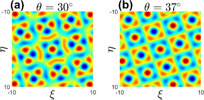
Figure 1. (a−b) The square Moiré lattice is formed by two sub-lattices with equal lattice depths (p1 = p2 = 1), each rotated by angles θ = 30° and θ = 37° (θ = arctan(3/4)), respectively, to create an external potential field. |
3. Soliton excited at the center of the potential field
We initiated our analysis by applying the numerical square operator iteration method to derive the soliton solution described in equation (3 ). Following this, we employed the split-step Fourier method to simulate the evolution of the soliton solution. Specifically, we examined how variations in the second sub-lattice depth p2 and the rotation angle θ between sub-lattices affected the soliton solution within the central Moiré lattice potential field (Δξ = Δη = 0).
In figures 2(a)–(b), we illustrate the distinct profiles of bright solitons observed at two different angles such that θ = 30° and θ = arctan(3/4) ≈ 37°, with both corresponding to p2 = 1. The variations in these angles are reflected in the distinct morphologies of the secondary peaks adjacent to the main peak of the bright soliton, exhibiting diverse symmetrical patterns relative to the soliton’s background (see figure 2, specifically 2(a3) and (b3)). On the other hand, we observe that as the gain and loss terms decrease, the stability of the solitons in the system degrades, even though the soliton waveforms remain unchanged. When the gain and loss terms are absent, the evolved soliton waveforms collapse immediately. Additionally, we noticed that as the rotation angle changes, increasing the depth of the second sub-lattice p2 not only clarifies the soliton background but also amplifies the peak amplitude and enhances the static stability of the soliton (see appendix A for details on how to judge soliton stability). Notably, when p2 = 1 and the soliton solution evolves over a duration of s = 1000, the change ${\left|{\rm{\Delta }}\varphi \right|}_{\max }$ approaches 0.01. This observation highlights the crucial role of the second sub-lattice depth p2 in shaping the formation and stability of soliton structures within the external potential landscape of the Moiré lattice.
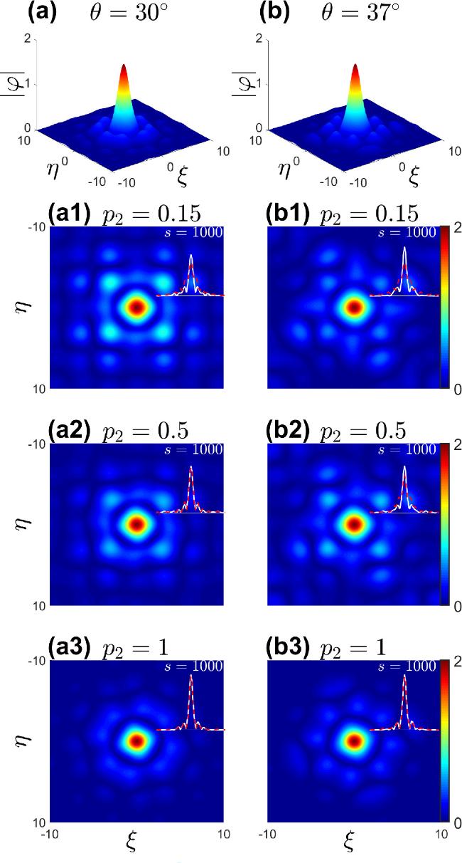
Figure 2. (a-b) When p1 = p2 = 1, there are stable soliton solutions under the Moiré lattice external potential fields at rotation angles θ = 30° and θ = 37°. (a1-a3) show top-down views of soliton solutions were depicted at the same angle θ = 30°, with respective values of p2 = 0.15 (a1), p2 = 0.5 (a2), and p2 = 1 (a3). Under this parameter setting, the insets depict a comparison of soliton profiles before and after soliton evolution (where η = 0). The solid white line represents the soliton profile before evolution, while the red dotted line represents the soliton profile after evolution, with an evolution duration of s = 1000. (b1-b3) follow the same format. |
To better understand this behavior, we delineated the regions where the rotation angle θ and the depth of the secondary sub-lattice p2 impact soliton stability, as illustrated in the θ-p2 region diagram shown in figure 3(a). In figure 3(a), Region I (red) indicates where the soliton solutions are statically stable; Region II (blue) highlights the areas of instability; Region III (orange) highlights the areas of bright vortex, dynamic bright vortex and dynamic soliton. From figures 3(b) to (g), we observe that the soliton background exhibits different symmetries at various angles, and the peak values are approximately same (${\left|\varphi \right|}_{\max }\approx 1.6$). The depth of the secondary sub-lattice is not the only factor influencing the morphology and stability of solitons. Our observations suggest that, at various angles, soliton solutions may lack static stability, even when p2 = 1. As illustrated in figure 3(d), the soliton solution becomes unstable at this angle due to ${\left|{\rm{\Delta }}\varphi \right|}_{\,\rm{max}\,}=0.13$ (for a detailed explanation of the soliton solution instability, refer to appendix A ). Furthermore, it is important to highlight Region III, where we identified bright vortices demonstrating both static and dynamic stability. The result of point (h) and (i) in figure 3(a) is shown in figure 4 and figure 5, respectively.
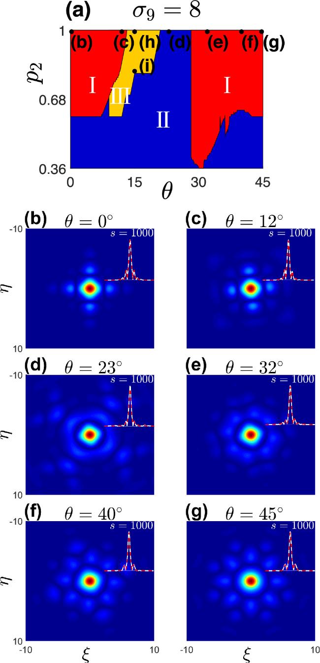
Figure 3. (a) The various solitons exist different regions under varying rotation angles θ and secondary sub-lattice depths p2: red Region I, blue Region II and orange Region III. (b-g) When p2 = 1, the top-view of the soliton at different rotation angles is shown, and the insets depicts a comparison of soliton profiles before and after soliton evolution (where η = 0). These solutions correspond to points (b-g) in diagrams (a). |
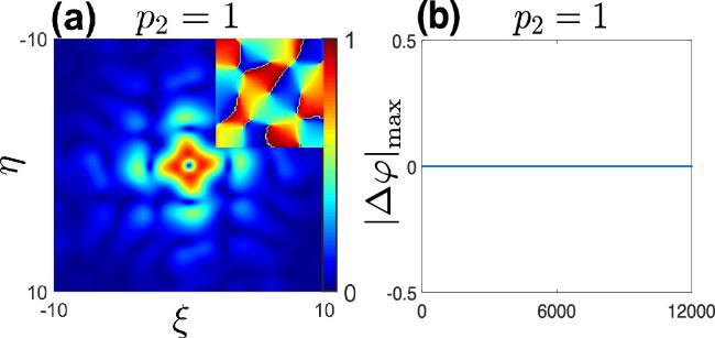
Figure 4. (a) For θ = 15° and p2 = 1, a top-down view of the square bright vortex soliton solution is presented, accompanied by an inset that illustrates the phase profiles of the square bright vortex soliton solution. (b) shows the changes in ${\left|{\rm{\Delta }}\varphi \right|}_{{\rm{\max }}}$ of the square bright vortex soliton solution during its evolution at s = 12000. This bright vortex result corresponds to the middle (h) point in figure 3(a). |
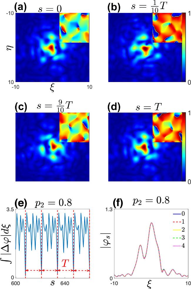
Figure 5. (a)–(d) For θ = 15° and p2 = 0.8, a top-down view of the square bright vortex soliton solution is presented and show the morphology of the bright vortex at different times within one period. These insets illustrate the phase profiles of the square bright vortex soliton. (e) shows the changes in $\int \left|{\rm{\Delta }}\varphi \right|d\xi $ of the square bright vortex soliton solution during its evolution at s = 12000. (f) shows the bright vortex profile along the ξ direction at a selected time s = 0 (the blue solid line, legend 0), compared with the soliton solution profiles after one (the red dotted line, legend 1), two (the yellow solid line, legend 2), three (the green dotted line, legend 3), and four (the purple dot line, legend 4) periods. The period is T = 13. This bright vortex result corresponds to the middle (i) point in figure 3(a). |
In figure 4, it is a statically stable bright vortex with a unique overall shape. Figure 4(b) shows the phase profiles of the solitons. It is evident that there is a 2π phase jump, which is a key characteristic of typical vortex structures. Additionally, figure 4(b) illustrates the changes in ${\left|{\rm{\Delta }}\varphi \right|}_{\max }$ of the square bright vortex soliton solution during its evolution. This is significant as it demonstrates the static stability of the bright vortex, which is explained in detail in appendix A . However, as shown in figures 5, when the depth of the second sub-lattice, represented by p2, is reduced to p2 = 0.8, we observe a rotating bright vortex. Figures 5(a)–(d), respectively, shows the evolution of an s = 0, $s=\,\frac{1}{10}T$, $s=\,\frac{9}{10}T$ and s = T when the top-view of the solitary wave solution. It is clear from these observations that the bright vortex is rotating throughout the evolution. Furthermore, figure 5(f) demonstrates that the soliton solutions overlap after every period, providing conclusive verification that the calculated period T = 13 is accurate. This periodic overlap highlights the reliability and consistency of the periodic stability observed in the dynamic soliton solutions. It can be seen that the second sublattice depth p2 is the key to change the static or dynamic state of solitons.
In our study of soliton solutions arising at the center of the Moiré lattice, we observed three distinct types, namely statically stable soliton solutions, dynamically stable soliton solutions, and unstable soliton solutions. To better understand the relationships among these solutions, we constructed region diagrams based on varying parameters such as θ and p2. For statically stable solutions, the square Moiré lattice, with its diverse external potentials, supports a richer variety of soliton backgrounds, including the presence of statically stable vortices. However, in the square Moiré lattice, these dynamically stable solutions are confined to a narrower range of rotation angles. In summary, we show that the modulation of solitons is strongly influenced by the rotation angle θ and the secondary lattice depth p2.
4. Soliton excited at the off-center of the potential field
In this section, we have excited soliton solutions within an off-center square external potential. The parameter we used is p2 = 1. We investigated the adjustment of soliton solutions under various rotation angles of the external potential using this parameter set. This process involved controlling the soliton solutions at different offset positions, expressed as V(r) = V(ξ + Δξ, η + Δη). In figure 6, we selected rotation angles of θ = 30° (quasi-periodic Moiré lattice potential) and θ = 37° (periodic Moiré lattice potential). Within a certain offset from the center of the external potential region, we identified two types of statically stable soliton solutions. When the rotation angle is set to θ = 30°, we observed statically stable solitons in small regions around the offsets Δξ = 10, Δη = 10; Δξ = 10, Δη = −10; Δξ = −10, Δη = 10; and Δξ = −10, Δη = −10. These solitons exhibited consistent shapes and occupied the same regions, differing only in their symmetry directions. As shown in figure 6(a), we selected the offset Δξ = −10 and Δη = 10 as the center to plot the red region where statically stable soliton solutions exist. The shape of these solitons is illustrated in figure 6(c). Similarly, at the rotation angle θ = 37°, the periodic pattern of the external potential (see figure 1(b)) allowed us to focus on a small periodic unit region. We selected the offset range Δξ ∈ [ −4, 4] and Δη ∈ [ −4, 4], and plotted the red region where statically stable soliton solutions exist (see figure 6(b)). The shapes of these soliton solutions are shown in figure 6(d). Unlike the soliton solutions excited at the center of the potential field, which can exhibit a rich variety of radial symmetries, we clearly observed that these soliton solutions are nearly uniaxially symmetric.
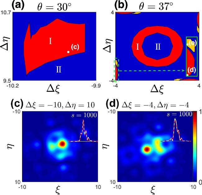
Figure 6. (a) When θ = 30°, in the vicinity of the region where the displacement from the external potential center is Δξ = − 10 and Δη = 10, statically stable solitons exist in the red region I. (b) When θ = 37°, in the vicinity of the region where the displacement from the external potential center is ${\rm{\Delta }}\xi \in \left[-4:\,4\right]$ and ${\rm{\Delta }}\eta \in \left[-4:\,4\right]$, statically stable solitons exist in the red Region I and periodic dynamic solitons exist in the orange Region. The inset shows an enlarged view of the area enclosed by the green dotted line. (c) When Δξ − 10 and Δη = 10, the statically stable soliton is shown, and the inset depicts a comparison of soliton profiles before and after soliton evolution. The solution correspond to points (c) in diagrams (a). (d) When Δξ = − 4 and Δη = − 4, the statically stable soliton is shown, and the inset depicts a comparison of soliton profiles before and after soliton evolution. The solution correspond to points (d) in diagrams (b). |
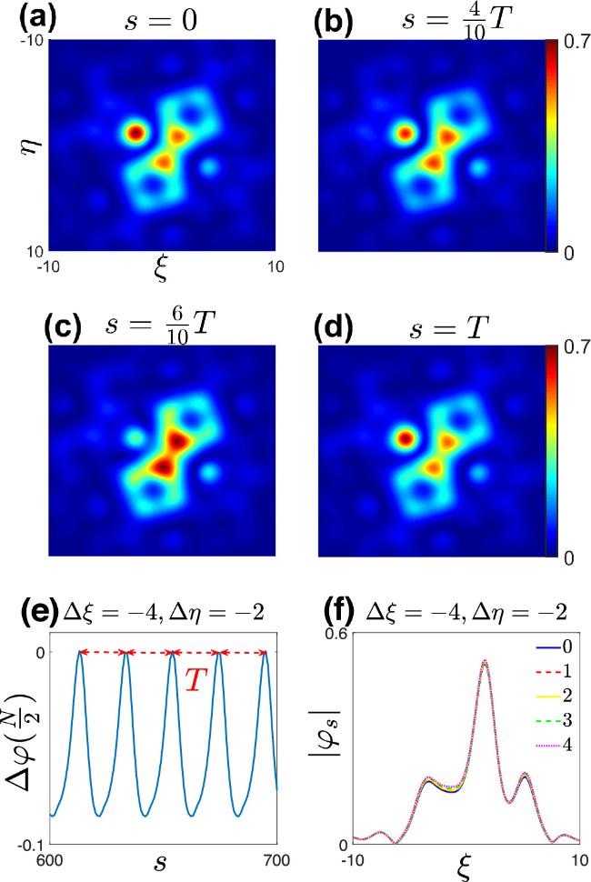
Figure 7. (a)–(d) When the rotation angle θ = 37°, a three-peak periodic dynamic soliton at the displacement from the external potential center Δξ= -4 and Δη= -2. And they show the morphology of the bright soliton at different times within one period. (e) shows the changes in ${\rm{\Delta }}\varphi (\frac{N}{2})$ of the soliton during its evolution at s = 12000. (f) shows the soliton profile along the ξ direction at a time s = 0, compared with the soliton profiles after one, two, three, and four periods. And T = 20. This periodic dynamic soliton corresponds to the (e) point in figure 6(b). |
As shown in figure 7, when the rotation angle is θ = 37°, we found a periodic dynamic stable soliton. This soliton exists in the orange region in figure 6(b). Unlike previously observed soliton configurations, these solutions exhibited a uniaxially symmetric three-peak structure, where two peaks are interconnected and the third remains isolated.
The dynamics of these solitons are particularly intriguing; when the amplitude of the isolated peak increases, the amplitude of the double peak decreases, and vice versa, resulting in periodic behavior akin to that of breathing solitons. The periodic changes are observed in figures 7(a)–(d), with a period of T = 20. For this dynamic soliton solution, as the gain and loss terms decrease, the original dynamic breathing solitons transform into static stable solitons, and the peak values of the soliton decrease. Even when the gain and loss terms are absent, the evolved soliton waveforms collapse directly.
Additionally, we have identified new periodic dynamic solitons within the range of external potential displacements at other rotation angles. When the rotation angle θ = 15°, we found periodic dynamic solitons only at the offset displacements Δξ = 0, Δη = 10; Δξ = 0, Δη = −10; Δξ = 10, Δη = 0; and Δξ = −10, Δη = 0.
As shown in figure 8, we selected the offset displacement Δξ = 0 and Δη = 10 to plot the shape of the periodic dynamic soliton. This solution corresponds to a four-peak soliton. Over time, the soliton peaks at the top and bottom, as well as those on the left and right, alternately merge and then separate again. The periodic changes of this soliton are shown in figures 8(a)–(d), with a period of T = 18.
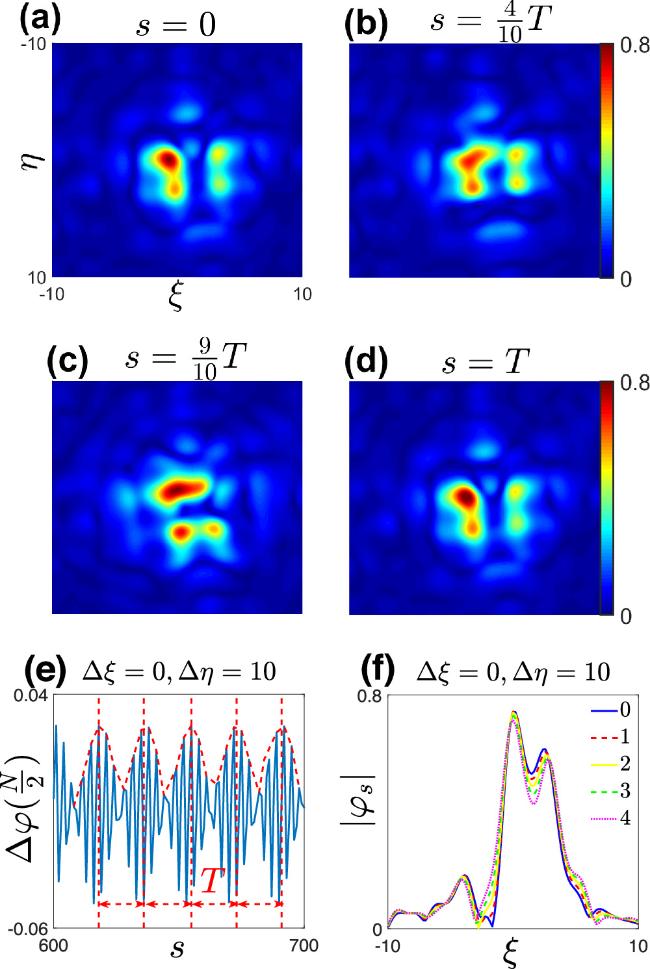
Figure 8. (a)–(d) When the rotation angle θ = 15°, a four-peak periodic dynamic soliton at the displacement from the external potential center Δξ = 0 and Δη = 10. And they show the morphology of the bright soliton at different times within one period. (e) shows the changes in ${\rm{\Delta }}\varphi \left(\frac{N}{2}\right)$ of the soliton during its evolution at s = 12000. (f) shows the soliton profile along the ξ direction at a time s = 0, compared with the soliton solution profiles after one, two, three, and four periods. And T = 18. |
Figures 9 and 10 illustrate two distinct types of dynamic soliton solutions observed at a rotation angle of θ = 45°, corresponding to specific offset displacements Δξ = 5, Δη = 5 and Δξ = 10, Δη = − 10. Interestingly, the soliton solutions corresponding to these displacements remain consistent across the four quadrants. In figure 9, we observe a uniaxially symmetric periodic dynamic five-peak soliton. In this soliton solution, the peaks in the northeast and southwest corners exhibit lower amplitudes, while the northwest, southeast, and central peaks are more prominent. As time progresses, the central peak merges with the southeast peak, resulting in a maximum combined amplitude. During this interaction, the amplitudes of the northeast and southwest peaks diminish. Eventually, the merged peak splits apart, allowing the amplitudes of the northeast and southwest peaks to recover and rise again. In figure 10(a), we observe a uniaxially symmetric periodic dynamic five-peak soliton. In this configuration, the northeast peak stands out with a higher amplitude, while the other peaks remain smaller. Over time, the peaks in the northeast, northwest, and southeast corners converge towards the center, resulting in a collision and merging at the center. As the amplitude of the northeast peak decreases, new soliton peak shapes emerge nearby (see figures 10(a)–(d). The central soliton then splits again, returning to its original positions in the northeast, northwest, and southeast corners, where the amplitudes increase, and the new soliton shapes vanish. At this rotation angle, the periods of the two breathing-type periodic dynamic solitons are T = 29 and T = 22, with both types exhibiting intriguing alternating behaviors.
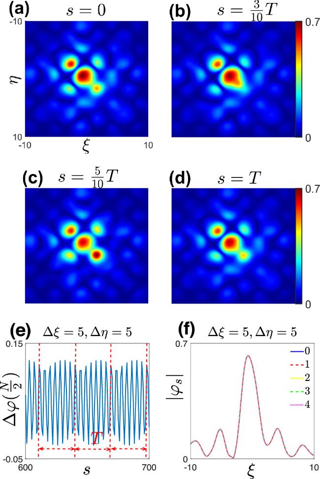
Figure 9. (a)–(d) When the rotation angle θ = 45°, a five-peak periodic dynamic soliton at the displacement from the external potential center Δξ = 5 and Δη = 5. And they show the morphology of the bright soliton at different times within one period. (e) shows the changes in ${\rm{\Delta }}\varphi \left(\frac{N}{2}\right)$ of the soliton during its evolution at s = 12000. (f) shows the soliton profile along the ξ direction at a time s = 0, compared with the soliton solution profiles after one, two, three, and four periods. And T = 29. |
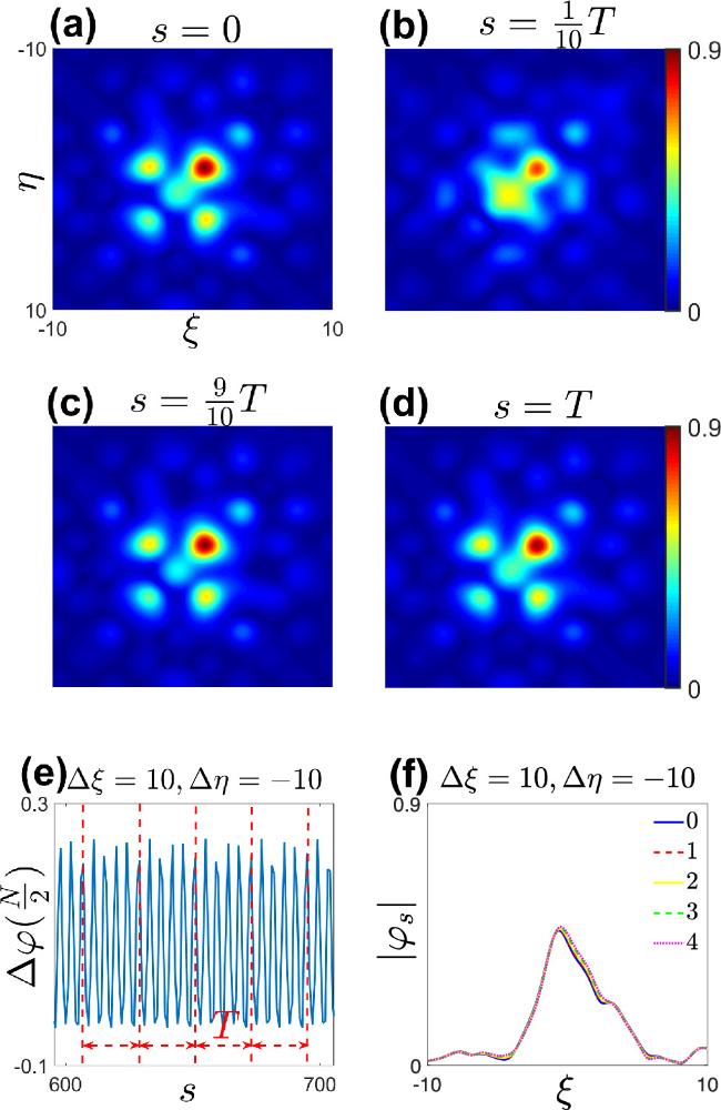
Figure 10. (a)–(d) When the rotation angle θ = 45°, a five-peak periodic dynamic soliton at the displacement from the external potential center Δξ = 10 and Δη = −10. And they show the morphology of the bright soliton at different times within one period. (e) shows the changes in ${\rm{\Delta }}\varphi \left(\frac{N}{2}\right)$ of the soliton during its evolution at s = 12000. (f) shows the soliton profile along the ξ direction at a time s = 0, compared with the soliton solution profiles after one, two, three, and four periods. And T = 22. |
The study revealed that under low pumping conditions, the initially unstable system tends to achieve dynamic equilibrium due to the influence of the Moiré lattice structure. The unique potential distribution, characterized by peak-valley asymmetry in the Moiré lattice, introduces an energy imbalance that facilitates multiple soliton excitations. This imbalance ultimately leads to the formation of diverse dynamic breathing multi-peak bright solitons. Under these low pumping conditions, the stable bright solitons are confined to a narrow parameter range, predominantly localized at the peaks of the Moiré lattice’s external potential. Additionally, our findings indicate that staggered multi-peak breathing bright solitons are more likely to emerge at non-periodic rotation angles, as shown in figures 9 and 10. In contrast, junction-bound multi-peak breathing bright solitons typically appear at periodic angles, as illustrated in figure 8.
5. Summary
In summary, we introduce a Moiré lattice external potential in a non-resonant, incoherently pumped exciton-polariton condensate system and propose schemes for realizing various forms of bright solitons, bright vortices, and periodic dynamic solitons. The composite pump consists of a uniform pump and a Gaussian pump, which together ensure gain-loss balance and maintain the soliton profile’s fundamental stability. We observe that in the Moiré potential field, variations in sub-lattice depths and rotation angles result in distinct background patterns in bright soliton solutions, with transitions between unstable and stable states. Furthermore, under specific conditions, we demonstrate effective modulation of both bright vortices and dynamic bright vortices. These findings highlight that sub-lattice depth and rotation angle in the Moiré potential play a crucial role in determining soliton characteristics. Additionally, we identify the parameter ranges required for the existence of different soliton solutions.
Regardless of their spatial placement in the external potential field, whether centered or off-center, a reduction in Gaussian pump intensity diminishes the system’s ability to maintain dynamic equilibrium. At this point, a Moiré potential with a high sub-lattice depth (typically requiring p2 = 1) becomes essential for achieving multi-peak soliton solutions. Under these conditions, stable bright solitons are constrained to a narrow parameter range, often corresponding to peak regions in the Moiré lattice’s external potential. Meanwhile, dynamic breathing multi-peak bright solitons align with regions between the peaks and valleys of the Moiré lattice. In addition, we also study the effects of pump amplitude σ9 and hexagonal Moiré lattice external potential on soliton properties in the system. These two parts are discussed in detail in appendix B and C . These findings substantially advance our understanding of the physical properties of exciton-polariton systems, providing a theoretical foundation for future experimental investigations, and hold significant potential for applications in quantum information science, optical switching, and quantum computing.
Appendix A. Relevant definitions of stable soliton
For various types of solitons, we employ the following evaluation methods. We define the initial soliton profile (where η = 0), obtained through iteration or evolution, as φ1, and the evolved soliton profile as φs, where the subscript s denotes the evolution time. The difference between the absolute values of these soliton profiles is expressed as Δφ = ∣φs∣ − ∣φ1∣. In the numerical calculation process, φ1 and φs are both data sets with N rows and 1 column.
If the system has statically stable solitons, the following two conditions must be satisfied. First, the maximum absolute value of Δφ corresponding to the soliton solution must be less than 0.1, i.e., ${\left|{\rm{\Delta }}\varphi \right|}_{max}\lt 0.1$. Second, the soliton waveform must remain unchanged during the evolution process. A soliton solution is considered unstable if it does not satisfy ${\left|{\rm{\Delta }}\varphi \right|}_{max}\lt 0.1$. As shown in figure 3(d), although the waveform of this soliton does not change significantly during evolution, ${\left|{\rm{\Delta }}\varphi \right|}_{\max }=0.13$, which does not meet the conditions, indicating instability.
If dynamically stable solitons exist in the system, the following two conditions must be met. First, the soliton solution must exhibit significant changes during the evolution process, such as rotation, breathing, etc., and these changes should be periodic or nearly periodic. To further verify this periodicity or near periodicity, we examine the corresponding ${\rm{\Delta }}\varphi (\frac{N}{2})$ of the soliton, which represents the difference between the values at a fixed position during the evolution of the soliton. If the difference ${\rm{\Delta }}\varphi (\frac{N}{2})$ repeatedly returns to zero over a period of time, this indicates that the soliton is able to return to its original position and coincide with its original form. The difference ${\rm{\Delta }}\varphi (\frac{N}{2})$ also exhibits periodic or near-periodic changes, which we define as T, the interval between solitons returning to their original position, i.e., the period.
It is worth noting that if the periodicity of ${\rm{\Delta }}\varphi (\frac{N}{2})$ over time is not sufficiently apparent, we can further calculate the change in $\int \left|{\rm{\Delta }}\varphi \right|{\rm{d}}\xi $ over time (as shown in figure 5(b)) and identify the time interval T for the periodic change. Additionally, if ${\rm{\Delta }}\varphi (\frac{N}{2})$ is clearly periodic over time, we can determine T by plotting its change envelope (as shown in figure 8(b)). The same approach applies to other solitons. Finally, we verify whether the soliton profile coincides over one cycle to confirm the correctness of T.
It is worth noting that in the above verification process of periodic dynamic soliton solutions, if the soliton solution returns to a static state and its ${\left|{\rm{\Delta }}\varphi \right|}_{max}\lt 0.1$, it also satisfies the condition for statically stable soliton solutions. As shown in figures 4(b), ${\left|{\rm{\Delta }}\varphi \right|}_{max}$ forms a straight line over time. We conclude that this soliton is a statically stable bright vortex.
Appendix B. The impact of Gaussian amplitude σ9
Our findings indicate that Gaussian pumping plays a significant role in soliton modulation, as illustrated in figure 11. A comparison between figures 11(c) and 4(a) reveals that a higher Gaussian pump amplitude (σ9 = 8) stabilizes the square vortex in a static state more effectively than a lower amplitude (σ9 = 5). However, for θ = 15° in figure 11(a), static stability is achieved only within a finite parameter range around σ9 = 9 and p2 = 1, as indicated by the single red point (I). In contrast to the broader parameter adjustment range provided by the Moiré lattice potential, the range of adjustment for the Gaussian pump amplitude is considerably narrower. For instance, as shown in figure 11(b), the static stability region for θ = 37° is confined to a very narrow Gaussian pump amplitude range, specifically σ9 ∈ [7.3, 10], with stability predominantly concentrated around σ9 = 8. On the other hand, dynamic solitons, as illustrated in figure 11(a), exhibit less stringent requirements for the Gaussian pump amplitude. They remain stable across a broader range of Gaussian pump amplitudes (σ9 ∈ [4, 10]).
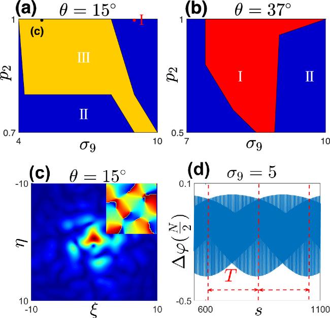
Figure 11. (a–b) When θ = 15° and θ = 37°, the various solitons exist different regions under varying secondary sub-lattice depths p2 and Gaussian amplitude σ9. (c) For θ = 15° p2 = 0.8 and σ9 = 5, a top-down view of the square periodic dynamic bright vortex soliton is presented. The inset shows the phase profiles of the bright vortex. The solution correspond to points (c) in diagrams (a). (d) shows the changes in ${\rm{\Delta }}\varphi (\frac{N}{2})$ of the periodic dynamic soliton during its evolution at s = 12000. And T = 223. |
Appendix C. The impact of the hexagonal Moiré lattice
We introduce hexagonal Moiré lattice into the system, which results in more stable solitons and periodic dynamic bright vortices. For the hexagonal lattice, it is expressed as ${V}_{1}({\boldsymbol{r}})={\sum }_{n=1}^{3}\cos (2\xi \cos {\theta }_{n}+2\eta \sin {\theta }_{n})$, where θ1 = 0, θ2 = 2π/3, and θ3 = 4π/3 (as shown in figure 12). As shown in figures 13(a)–(b), we have plotted the regions of existence for various soliton states by examining two additional parameters under the conditions of a Gaussian pump amplitude σ9 = 8 and rotation angle θ = 30°. Our findings reveal that statically stable solitons are highly sensitive to variations in the Gaussian pump amplitude, with their existence confined to the range σ9 ∈ [6, 10]. Notably, statically stable solitons maintain static stability over the largest p2 interval exclusively when σ9 = 8.
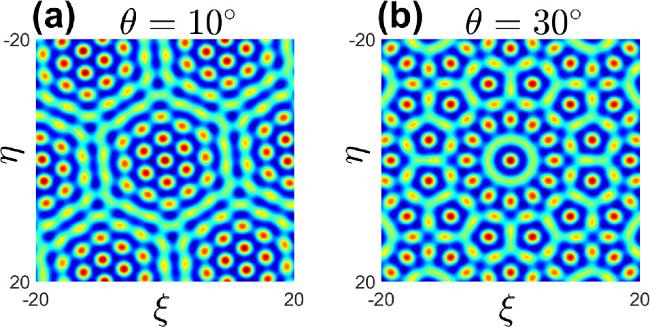
Figure 12. (a–b) The hexagonal Moiré lattice is formed by two sub-lattices with equal lattice depths (p1 = p2 = 1), each rotated by angles θ = 10° and θ = 30°, respectively, to create an external potential field. |
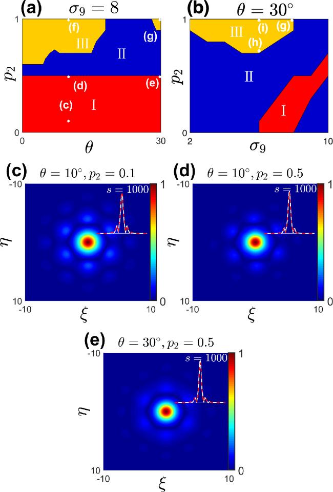
Figure 13. (a-b) When σ9 = 8 and θ = 30°, the various solitons exist different regions. (c-d) When θ = 10° and σ9 = 8, the top-view of the soliton at different p2 is shown, and the insets depicts a comparison of soliton profiles before and after soliton evolution. These solutions correspond to points (c) and (d) in diagram (a). (e)When θ = 30°, σ9 = 8 and p2 = 0.5, the top-view of the soliton is shown, and the insets depicts a comparison of soliton profiles before and after soliton evolution. The solution correspond to points (e) in diagram (a). |
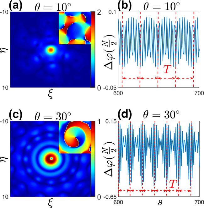
In contrast, periodic dynamic soliton solutions persist across most of the Gaussian pump amplitude interval. By comparing figure 13(d) (θ = 10°) and (e) (θ = 30°), we can find that there are solitons of different shapes at different rotation angles. This further highlights the modulation of the system solitons by the rotation angle. Figures 13(c–d) show the soliton background becomes more distinct at higher secondary lattice depth p2. This behavior is further demonstrated in figure 14(a) (p2 = 0.7) and (c) (p2 = 1) while θ = 30°. With the increase of p2, the periodic rotating bright vortices in the system become clearer and clearer. As shown in figure 14(c), when p2 = 1, different forms of periodic rotating bright vortices appear in the system. As shown in figure 15, dynamic bright vortices of different shapes will also appear at different rotation angles. Notably, all dynamically stable solutions exhibit rotational behavior throughout their evolution. In contrast, in hexagonal Moiré lattices external potential, statically stable soliton solution structures are more uniform and occupy a larger parameter space, i.e. exist at all rotation angles. On the other hand, in the hexagonal Moiré lattice external potential, periodic dynamic vortices show regular morphological changes.
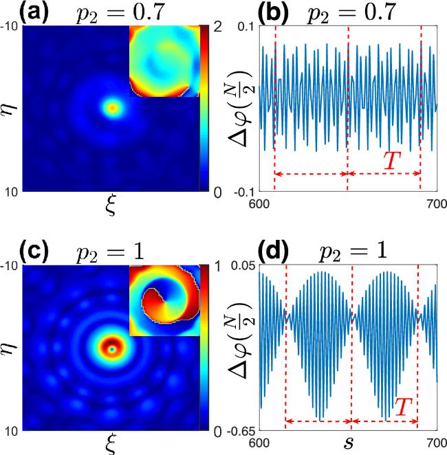
Figure 14. (a), (c) show two periodic dynamic bright vortices, while θ = 30° and σ9 = 6. The insets show the phase profiles of the bright vortices. These solutions correspond to points (h) and (i) in figure 13(b). (b) shows the changes in ${\rm{\Delta }}\varphi (\frac{N}{2})$ of the periodic dynamic vortex (a) during its evolution at s = 12000. And T = 41. (d) shows the changes in ${\rm{\Delta }}\varphi (\frac{N}{2})$ of the periodic dynamic vortex (c) during its evolution at s = 12000. And T = 37. |
Figure 15. (a), (c) show two periodic dynamic bright vortices, while p2 = 1 and σ9 = 8. The insets show the phase profiles of the bright vortices. These solutions correspond to points (f) and (g) in figure 13(a). (c) also correspond to points (g) in figure 13(b). (b) shows the changes in ${\rm{\Delta }}\varphi (\frac{N}{2})$ of the periodic dynamic vortex (a) during its evolution at s = 12000. And T = 22. (d) shows the changes in ${\rm{\Delta }}\varphi (\frac{N}{2})$ of the periodic dynamic vortex (c) during its evolution at s = 12000. And T = 15. |