


1. Introduction
Nonlinear science [1, 2] encompasses a broad spectrum of research fields within both natural and social sciences, encompassing disciplines such as mathematics [3, 4], chemistry [5], biology [6], earth science [7], physics [8, 9], economics [10] and other pivotal areas. Its core mission is to establish bridges between mathematics and these various disciplines. Linear systems typically adhere to the principles of homogeneity and superposition, where the latter allows for straightforward analysis by considering the cumulative effect of individual stimuli as the sum of their separate responses. Conversely, nonlinear systems generally do not conform to the principle of superposition. The essence of linearity often represents an idealization of the complex real world, where multiple influencing factors must be taken into account. Consequently, there is a pressing need to delve into the development of nonlinear science to better understand and model the intricate phenomena observed in nature and society.
The quest for exact solutions to high-dimensional nonlinear evolution equations has long been a focal point for researchers, as these solutions provide invaluable insights into the underlying physical phenomena. A multitude of methods exist for tackling nonlinear systems, including the Darboux transformation method [11, 12], the variable separation approach [13], the auxiliary equation technique [14], the bilinear neural network method [15], the bilinear residual network method [16], the nonlinear superposition formula [17], the (G/G)-expansion method [18] and the weighted residual method [19]. Each of these methodologies offers a unique perspective and set of tools for deriving precise analytical solutions to complex nonlinear equations.
Transforming nonlinear evolution equations into a bilinear form constitutes a powerful approach for studying nonlinear problems. In the realm of bilinear methods for nonlinear evolution equations, two notable techniques are the Bell polynomial method [20–22] and the Hirota bilinear method [23–30]. The Hirota bilinear method achieves the bilinear form of nonlinear evolution equations through the introduction of transformations. In contrast, the Bell polynomial method not only yields the bilinear form of these equations but also derives corresponding bilinear Bäcklund transformations, Lax pairs, conservation laws, and more, thereby facilitating the analysis of the integrability of the nonlinear system. Furthermore, by leveraging the bilinear Bäcklund transformation of the equation, one can obtain the nonlinear superposition formula for the solution of the equation, which in turn enables the derivation of infinite superposition solutions using this formula.
In this paper, we will study a (3+1)-dimensional Calogero–Bogoyavlenskii–Schiff (CBS) equation 1 ) through the the Hirota method and symbolic computation [31]. The N-soliton solutions composed of the higher-order breather, periodic line wave and the mixed forms were studied by the Hirota bilinear method and the rational and semi-rational solutions of the equation were acquired by using complex conjugate parameter relations and the long-wave limit method [32].
$\begin{eqnarray}\begin{array}{rcl} & & {u}_{t}-{l}_{1}(u{u}_{y}+{u}_{x}{\partial }_{x}^{-1}{u}_{y})-{l}_{2}u{u}_{z}-{l}_{3}{u}_{xxy}-{l}_{4}{u}_{xxz}+{l}_{5}{u}_{x}\\ & & +{\partial }_{x}^{-1}{u}_{yy}+{l}_{7}{\partial }_{x}^{-1}{u}_{zz}-{l}_{8}{u}_{x}{\partial }_{x}^{-1}{u}_{z}=0,\end{array}\end{eqnarray}$
where l1, l2, …, l8 are nonzero constants and u is a function of variables x, y, z and t. The lump, mixed lump-stripe, mixed rogue wave-stripe and breather wave solutions of equation (If the parameters l1 = a = b, l2 = l8 = − c, l3 =l4 = − 1, l5 = l6 = l7 = 0, then equation (1 ) will be turned out (2 ) given as
$\begin{eqnarray}\begin{array}{rcl} & & {u}_{t}-au{u}_{y}+b{u}_{x}{\partial }_{x}^{-1}{u}_{y}\\ & & +cu{u}_{z}+{u}_{xxy}+{u}_{xxz}+c{u}_{x}{\partial }_{x}^{-1}{u}_{z}=0,\end{array}\end{eqnarray}$
based on the Cole–Hopf transformation and the Hirota bilinear method to derive multiple soliton solutions and multiple singular soliton solutions for these equations [33]. We obtain commutator table of through Lie brackets and symmetry groups for the CBS equation and obtain closed-form solutions of the CBS equation by using the invariance property of Lie group transformations [34].If the parameters ${l}_{1}=1,{l}_{4}=\frac{1}{4}$,${l}_{8}=\frac{1}{2}$,l1 = l3 = l5 =l7 = 0, then equation (1 ) will be turned out (2+1)-dimensional potential Yu–Toda–Sa–Fukuyama (YTSF) equation,
$\begin{eqnarray}{u}_{t}-u{u}_{z}-\frac{1}{4}{u}_{xxz}-\frac{3}{4}{\partial }_{x}^{-1}{u}_{yy}-\frac{1}{2}{u}_{x}{\partial }_{x}^{-1}{u}_{z}=0.\end{eqnarray}$
Weierstrass elliptic function solutions are investigated by applying the traveling wave transformation and auxiliary equations to a (2+1)-dimensional potential (YTSF) equation [35].
Compared to the existing literature, it is essential to consider both the equation and its compatibility conditions concurrently when utilizing the Bell polynomial method. It is noteworthy that our work transcends merely obtaining the bilinear form of equation (1 ) using the Bell polynomial method. We also deduce several crucial properties, including the bilinear Bäcklund transformation, Lax pair, infinite conservation laws and the nonlinear superposition formula. Furthermore, we have demonstrated that equation (1 ) is completely integrable in the sense of the Lax pair.
It is emphasized that this paper not only extracts a multitude of properties via the Bell polynomial method but also constructs a nonlinear superposition formula for the CBS equation. By applying this nonlinear superposition principle, we obtain infinite superposition solutions for the equation. Through this research, we not only deepen our understanding of nonlinear wave phenomena but also offer new perspectives and methodologies for future scientific endeavors.
The structure of the paper will be organized as follows: in section 2 , we will present the definition and properties of Bell polynomials. In section 3 , we will derive the bilinear form of equation (1 ). In section 4 , we will discuss the bilinear Bäcklund transformation, Lax pairs, and the integrability of equation (1 ) in the sense of the Lax pair. In section 5 , we will obtain infinite conservation laws for equation (1 ). In section 6 , we will derive the nonlinear superposition formula for equation (1 ). In section 7 , we will explore superposition wave solutions and utilize the symbolic calculation system Mathematica to draw three-dimensional maps, contour maps, and line plots in order to analyze their dynamic characteristics.
2. Definition and properties of Bell polynomials
First, the concept and properties of Bell polynomials are briefly introduced.
The first type of Bell polynomial is defined as
$\begin{eqnarray}{\xi }_{0}(x,t,r)={{\rm{e}}}^{-t{x}^{r}}{\partial }_{x}^{n}{{\rm{e}}}^{t{x}^{r}},\end{eqnarray}$
which r is a constant, n is any integer, x and t are independent variables.The second type of Bell polynomial φn is a polynomial about α1, · · · , αn, which is defined as
$\begin{eqnarray}{\phi }_{n}=\phi ({\alpha }_{1},\cdot \cdot \cdot ,{\alpha }_{n}),{\phi }_{0}=1,{\phi }_{n+1}\displaystyle \sum _{s=1}^{n}\left(\frac{n}{s}\right){\alpha }_{s+1}{\phi }_{n-s},\end{eqnarray}$
where (α1, · · · , αn) is an infinite sequence of variables independent.The third type of Bell polynomial is a generalization of the first and second type of Bell polynomials, which are defined as
$\begin{eqnarray}{Y}_{n}={Y}_{n}({y}_{t},\cdot \cdot \cdot ,{y}_{nt})={{\rm{e}}}^{-y}{\partial }_{t}^{n}{{\rm{e}}}^{y},\end{eqnarray}$
including $y={{\rm{e}}}^{\alpha t}-{\alpha }_{0}\equiv {\alpha }_{1}t+\frac{{\alpha }_{2}{t}^{2}}{2!}+\cdot \cdot \cdot $, and the third type of Bell polynomial is the function of y and the first few low-order polynomials of the third type of Bell polynomial are given below $\begin{eqnarray}{Y}_{0}={f}_{x},{Y}_{1}={y}_{t},{Y}_{2}={y}_{y}^{2}+{y}_{2t},{Y}_{3}={f}_{t}^{3}+3{y}_{t}{y}_{2t}+{y}_{3t},\cdot \cdot \cdot \end{eqnarray}$
The third type of Bell polynomial is extended to multidimensionality, which is closely related to bilinear equations, and its definition and correlation properties are introduced next.
Definition 1.Assuming that f = f(x1, x2, · · · , xn) is a function on ${{\mathbb{C}}}^{\infty }$,
$\begin{eqnarray}\begin{array}{l}{Y}_{{n}_{1}{x}_{1},{n}_{2}{x}_{2},\cdot \cdot \cdot ,{n}_{r}{x}_{r}}(f)\\ \equiv {Y}_{{n}_{1}{x}_{1},{n}_{2}{x}_{2},\cdot \cdot \cdot ,{n}_{r}{x}_{r}}({f}_{{l}_{1}{x}_{1}},{f}_{{l}_{2}{x}_{2}},\cdot \cdot \cdot ,{f}_{{l}_{r}{x}_{r}})={{\rm{e}}}^{-f}{\partial }_{{x}_{1}}^{{n}_{1}}\cdot \cdot \cdot {\partial }_{{x}_{r}}^{{n}_{r}}{{\rm{e}}}^{f},\end{array}\end{eqnarray}$
is called the Bell polynomial, which is simply denoted as the Y-polynomial.Eg1: we can calculate the initial explicit expressions by the definition as follows
$\begin{eqnarray}\begin{array}{rcl}{Y}_{1x}(f) & = & {f}_{x},{Y}_{2x}(f)={f}_{2x}+{f}_{x}^{2},\\ {Y}_{3x}(f) & = & {f}_{3x}+3{f}_{x}{f}_{2x}+{f}_{x}^{3},\cdot \cdot \cdot \end{array}\end{eqnarray}$
Eg2: as for a special function f with the variables x, y, we give rise to the following several initial values under the definition of the Bell polynomial.
$\begin{eqnarray}{Y}_{x,t}(f)={f}_{x,t}+{f}_{x}{f}_{t},{Y}_{2x,t}(f)={f}_{2x,y}+{f}_{2x}{f}_{t}+{f}_{x}^{2}{f}_{t},\cdot \cdot \cdot \end{eqnarray}$
Definition 2.In the view of the multivariables Bell polynomial, the Bell polynomial can be defined as follows
$\begin{eqnarray}{{ \mathcal Y }}_{{n}_{1}{x}_{1},\cdot \cdot \cdot ,{n}_{l}{x}_{l}}(v,w)={Y}_{{n}_{1}\cdot \cdot \cdot ,{n}_{l}}({f}_{{n}_{1}{x}_{1},\cdot \cdot \cdot ,{n}_{l}{x}_{l}}),\end{eqnarray}$
where w and v both are the ${{\mathbb{C}}}^{\infty }$ function with the variables x1, · · · , xl, $\begin{eqnarray}{f}_{{r}_{1}{x}_{1},\cdot \cdot \cdot ,{r}_{l}{x}_{l}}=\left\{\begin{array}{l}{v}_{{n}_{1}{x}_{1}},{l}_{1}{x}_{1},{l}_{1}+\cdot \cdot \cdot +{l}_{r}=\mathrm{odd},\\ {w}_{{n}_{1}{x}_{1}},{l}_{1}{x}_{1},{l}_{1}+\cdot \cdot \cdot +{l}_{r}=\mathrm{even}.\end{array}\right..\end{eqnarray}$
The first few low-order double Bell polynomials $\begin{eqnarray}\begin{array}{rcl}{{ \mathcal Y }}_{x}(v,w) & = & {v}_{x},{{ \mathcal Y }}_{2x}(v,w)={v}_{x}^{2}+{w}_{2x},{{ \mathcal Y }}_{3x}(v,w)={v}_{x}^{3}+3{v}_{x}{w}_{2x}+{v}_{3x},\\ {{ \mathcal Y }}_{x,t}(v,w) & = & {v}_{x}{v}_{y}+{w}_{xt}{{ \mathcal Y }}_{4x}(v,w)={w}_{4x}+4{v}_{x}{v}_{3x}+6{v}_{x}^{2}{w}_{2x}+{v}_{x}^{4},\cdot \cdot \cdot \end{array}\end{eqnarray}$
Theorem 1.Bell polynomial (
$\begin{eqnarray}{{ \mathcal Y }}_{{n}_{1}{x}_{1},\cdot \cdot \cdot ,{n}_{r}{x}_{x}}({\mathrm{ln}}\,\frac{F}{G},FG)={(FG)}^{-1}{D}_{{x}_{1}}^{{n}_{1}}\cdot \cdot \cdot {D}_{{x}_{r}}^{{n}_{r}}F\cdot G,\end{eqnarray}$
which is n1 + n2 + n3 + · · · nr≥1.When F = G the relation (14) can use the following formula to redefine
$\begin{eqnarray}\begin{array}{rcl} & & {(FG)}^{-1}{D}_{{x}_{1}}^{{n}_{1}}\cdot \cdot \cdot {D}_{{x}_{r}}^{{n}_{r}}F\cdot G\\ & = & \left\{\begin{array}{l}0,{n}_{1}+\cdot \cdot \cdot +{n}_{r}=\mathrm{odd},\\ {P}_{{n}_{1}{x}_{1},\cdot \cdot \cdot ,{n}_{r}{x}_{r}}(q),{n}_{1}+\cdot \cdot \cdot +{n}_{r}=\mathrm{even}.\end{array}\right.\end{array}\end{eqnarray}$
The following equation is called the P-polynomial $\begin{eqnarray}{P}_{{n}_{1}{x}_{1},\cdot \cdot \cdot ,{n}_{l}{x}_{l}}(q)={{ \mathcal Y }}_{{n}_{1}{x}_{1},\cdot \cdot \cdot ,{n}_{l}{x}_{l}}(0,q=2\,{\mathrm{ln}}\,F),\end{eqnarray}$
only if n1 + n2 + , · · · , + nl is an even number.3. Bilinear form
By transforming nonlinear partial differential equations into a bilinear form, by solving bilinear equations, exact solutions can be generated. In this section, we will use Bell polynomial method to obtain the bilinear form of the equation (1 ).
Make transformation
$\begin{eqnarray}u=c{q}_{xx},\end{eqnarray}$
where c is an arbitrary constant.Substituting equation (17 ) into equation (1 ), taking c = 1, with l1 = 3l3, l2 = l8 = 3l4,19 ) can be expressed by the P-polynomial as 1 ) is obtained
$\begin{eqnarray}\begin{array}{rcl} & & {q}_{xxt}-3{l}_{3}({q}_{xx}{q}_{xxy}+{q}_{xxx}{q}_{xy})\\ & & -3{l}_{4}{q}_{xx}{q}_{xxz}-{l}_{3}{q}_{xxxxy}-{l}_{4}{q}_{xxxxz}\\ & & +{l}_{5}{q}_{xxx}+{l}_{6}{q}_{xyy}+{l}_{7}{q}_{xzz}-3{l}_{4}{q}_{xxx}{q}_{zx}=0,\end{array}\end{eqnarray}$
integrate equation with variable x once and make the integral constants as zero to obtain $\begin{eqnarray}\begin{array}{rcl} & & {q}_{xt}-3{l}_{3}{q}_{xx}{q}_{xy}-3{l}_{4}{q}_{xx}{q}_{xz}-{l}_{3}{q}_{xxxy}-{l}_{4}{q}_{xxxz}\\ & & +{l}_{5}{q}_{xx}+{l}_{6}{q}_{yy}+{l}_{7}{q}_{zz}=0.\end{array}\end{eqnarray}$
According to the correlation properties of the P-polynomial, $\begin{eqnarray}\begin{array}{rcl}{P}_{2x}(q) & = & {q}_{2x},{P}_{xt}(q)={q}_{xt},{P}_{4x}(q)\\ & = & {q}_{4x}+3{q}_{2x}^{2},{P}_{3t,x}(q)={q}_{3t,x}+3{q}_{2t}{q}_{xt}.\end{array}\end{eqnarray}$
Equation ( $\begin{eqnarray}{P}_{xt}-{l}_{3}{P}_{3x,y}-{l}_{4}{P}_{3x,z}+{l}_{5}{P}_{xx}+{l}_{6}{P}_{yy}+{l}_{7}{P}_{zz}=0.\end{eqnarray}$
From the relationship between the double Bell polynomial and the Hirota linear term, the bilinear form of equation ( $\begin{eqnarray}({D}_{x}{D}_{t}-{l}_{3}{D}_{x}^{3}{D}_{y}-{l}_{4}{D}_{x}^{3}{D}_{z}+{l}_{5}{D}_{x}^{2}+{l}_{6}{D}_{y}^{2}+{l}_{7}{D}_{z}^{2})f\cdot f=0.\end{eqnarray}$
4. Bilinear Bäcklund transformation and Lax pair
In order to obtain the Bäcklund transformation of the equation, let and be two different solutions of equation (19 ), respectively, and substitute the two solutions into the equation and perform algebraic operations, as follows23 ) can be rewritten as follows 25 ) constant zero, the Bäcklund transform of the Bell polynomial of the equation is obtained by combining the correlation method
$\begin{eqnarray}\begin{array}{rcl} & & E(\bar{q})-E(q)\\ & = & -2{l}_{3}[3({\bar{q}}_{xx}{\bar{q}}_{xy}-{q}_{xx}{q}_{xy})+{(\bar{q}-q)}_{xxxy}]\\ & & -2{l}_{4}[3({\bar{q}}_{xx}{\bar{q}}_{xz}-{q}_{xx}{q}_{xz})\\ & & +{(\bar{q}-q)}_{xxxz}]2{(\bar{q}-q)}_{xt}+2{l}_{5}{(\bar{q}-q)}_{xx}\\ & & +2{l}_{6}{(\bar{q}-q)}_{yy}+2{l}_{7}{(\bar{q}-q)}_{zz}=0.\end{array}\end{eqnarray}$
Two new variables have been introduced $\begin{eqnarray}v=\frac{(\bar{q}-q)}{2}={\mathrm{ln}}\,F/G,w=\frac{(\bar{q}+q)}{2}={\mathrm{ln}}\,FG.\end{eqnarray}$
Then ( $\begin{eqnarray}\begin{array}{rcl}E(w+v)-E(w-v) & = & 2\{-{l}_{3}[3({v}_{yx}{w}_{xx}-{w}_{yx}{v}_{xx})+{v}_{xxxy}]\\ & & -{l}_{4}[3({v}_{zx}{w}_{xx}-{w}_{zx}{v}_{xx})+{v}_{xxxz}]+{v}_{xt}+{l}_{5}{v}_{xx}+{l}_{6}{v}_{yy}+{l}_{7}{v}_{zz}\}\\ & = & 2[{\partial }_{x}({l}_{5}{{ \mathcal Y }}_{x}+{{ \mathcal Y }}_{t})-{\partial }_{y}({l}_{3}{{ \mathcal Y }}_{3x}-{l}_{6}{{ \mathcal Y }}_{y})+{\partial }_{z}({l}_{4}{{ \mathcal Y }}_{3x}-{l}_{7}{{ \mathcal Y }}_{z})]\\ & & +{Q}_{1}(v,w)+{Q}_{2}(v\,\rm{,w}\,)=0.\end{array}\end{eqnarray}$
where ${Q}_{1}(v,w)\,=\,6W[{{ \mathcal Y }}_{x}(v,\,w),\,{{ \mathcal Y }}_{x,y}(v,\,w)],{Q}_{2}(v,w)\,=6W[{{ \mathcal Y }}_{x}(v,w),{{ \mathcal Y }}_{x,z}(v,w)].$ In order to make equation ( $\begin{eqnarray}\begin{array}{c}\left\{\begin{array}{c}{{ \mathcal Y }}_{{xy}}=\lambda {{ \mathcal Y }}_{x},\\ {{ \mathcal Y }}_{{xz}}=\lambda {{ \mathcal Y }}_{x,}\\ {l}_{3}{{ \mathcal Y }}_{3x}-{l}_{6}{{ \mathcal Y }}_{y}-\lambda =0,\\ {l}_{4}{{ \mathcal Y }}_{3x}-{l}_{7}{{ \mathcal Y }}_{z}-\lambda =0,\\ {{ \mathcal Y }}_{t}+{l}_{5}{{ \mathcal Y }}_{x}-\lambda =0,\end{array}\right.\end{array}\end{eqnarray}$
where λ is an arbitrary constant.From the relationship between polynomial and bilinear operator, the bilinear Bäcklund transform of equation (1 ) is obtained,28 ) into equation (26 ) gets
$\begin{eqnarray}\left\{\begin{array}{l}({D}_{x}{D}_{y}-\lambda {D}_{x})F\cdot G=0,\\ ({D}_{x}{D}_{z}-\lambda {D}_{x})F\cdot G=0,\\ ({l}_{3}{D}_{x}^{3}-{l}_{6}{D}_{y}-\lambda )F\cdot G=0,\\ ({l}_{4}{D}_{x}^{3}-{l}_{7}{D}_{z}-\lambda )F\cdot G=0,\\ ({D}_{t}+{l}_{5}{D}_{x}-\lambda )F\cdot G=0.\end{array}\right.\end{eqnarray}$
Based on the Hopf–Cole transformation, making v = lnψ, derives the following expression from the properties of the ${ \mathcal Y }-$ polynomial: $\begin{eqnarray}\begin{array}{rcl}{{ \mathcal Y }}_{x}(v) & = & \frac{{\psi }_{x}}{\psi },{{ \mathcal Y }}_{t}(v)=\frac{{\psi }_{t}}{\psi },{{ \mathcal Y }}_{y}(v)=\frac{{\psi }_{y}}{\psi },{{ \mathcal Y }}_{2x}(v,w)={q}_{2x}+\frac{{\psi }_{2x}}{\psi },\\ {{ \mathcal Y }}_{x,y}(v,w) & = & \frac{{\psi }_{x,y}}{\psi }+{q}_{xy},{{ \mathcal Y }}_{3x}(v,w)=\frac{{\psi }_{3x}}{\psi }+3{q}_{2x}\frac{{\psi }_{x}}{\psi }.\end{array}\end{eqnarray}$
Substituting equation ( $\begin{eqnarray}\left\{\begin{array}{l}\lambda {\psi }_{x}={\psi }_{xy}+{q}_{xy}\psi ,\\ \lambda {\psi }_{x}={\psi }_{xz}+{q}_{xz}\psi ,\\ {l}_{3}{\psi }_{3x}+3{l}_{3}{q}_{2x}{\psi }_{x}-{l}_{6}{\psi }_{y}=\lambda \psi ,\\ {l}_{4}{\psi }_{3x}+3{l}_{4}{q}_{2x}{\psi }_{x}-{l}_{7}{\psi }_{z}=\lambda \psi ,\\ {\psi }_{t}+{l}_{5}{\psi }_{x}=\lambda \psi .\end{array}\right.\end{eqnarray}$
The first and second sub-formulas in (29 ) are substituted into the other formulas, we can get
$\begin{eqnarray}\left\{\begin{array}{l} {\left[\partial_{t}+L_{1}\right] \psi=\left[\partial_{t}+l_{3} \partial_{x}^{3}+3 l_{3} q_{2 x} \frac{\partial_{x} \partial_{y}+q_{x y}}{\lambda}-l_{6} \partial_{y}+l_{5} \partial_{x}-2 \lambda\right] \psi,} \\ {\left[L_{2}-\lambda\right] \psi=\left[l_{4} \partial_{x}^{3}+3 l_{4} q_{2 x} \frac{\partial_{x} \partial_{z}+q_{x z}}{\lambda}-l_{7} \partial_{z}-\lambda\right] \psi .} \end{array}\right.\end{eqnarray}$
The Lax pair of equations satisfies [∂t + L1, L2 − λ] = 0, where ${L}_{2}={l}_{4}{\partial }_{x}^{3}+3{l}_{4}{q}_{2x}\frac{{\partial }_{x}{\partial }_{z}+{q}_{xz}}{\lambda }-{l}_{7}{\partial }_{z},{L}_{1}={l}_{3}{\partial }_{x}^{3}+3{l}_{3}{q}_{2x}\frac{{\partial }_{x}{\partial }_{y}+{q}_{xy}}{\lambda }-{l}_{6}{\partial }_{y}+{l}_{5}{\partial }_{x}-2\lambda .$
In the transformation of bilinear representation, the product is satisfied by replacing u with which happens to be equation (1 ).
5. Infinite conservation laws
From the relation ${\partial }_{x}{{ \mathcal Y }}_{y}={\partial }_{y}{{ \mathcal Y }}_{x}={v}_{xy}$, then the formula (26) can be rewritten as 32 ) into equation (31 ), we get 33 ) and (34 ), we expand the function into the following series 35 ) compares the power coefficient of ϵ to obtain the recursive relation of the conserved density In35 ) into the (34 ) formula
$\begin{eqnarray}\left\{\begin{array}{l}{w}_{xy}+{v}_{x}{v}_{y}-\lambda {v}_{x}=0,\\ {w}_{xz}+{v}_{x}{v}_{z}-\lambda {v}_{x}=0,\\ {\partial }_{x}[({l}_{3}+{l}_{4})({v}_{3x}+3{v}_{x}{w}_{2x}+{v}_{x}^{3})+{v}_{t}+{l}_{5}{v}_{x}+{l}_{6}{v}_{y}-{l}_{7}{v}_{z}]=0.\end{array}\right.\end{eqnarray}$
Introducing potential function $\eta =\frac{{q}_{x}^{{}^{{\prime} }}-{q}_{x}}{2}$, according to the transformation (24), we get $\begin{eqnarray}{v}_{x}=\eta ,{w}_{x}={q}_{x}+\eta .\end{eqnarray}$
Substituting formulas ( $\begin{eqnarray}{\eta }_{y}+\eta {\partial }_{x}^{-1}{\eta }_{y}+{q}_{xy}-\lambda \eta =0,\end{eqnarray}$
and a discrete equation $\begin{eqnarray}\begin{array}{rcl} & & ({l}_{3}+{l}_{4}){\partial }_{x}({\eta }_{xx}+3\eta {q}_{xx}+3\eta {\eta }_{x}+{\eta }^{3})+{\eta }_{t}\\ & & +{l}_{5}{\eta }_{x}+{l}_{6}{\eta }_{y}-{l}_{7}{\eta }_{z}=0.\end{array}\end{eqnarray}$
To balance equations ( $\begin{eqnarray}\eta =\varepsilon +\displaystyle \sum _{n=1}^{\infty }{I}_{n}(q,{q}_{x},\cdots \,){\varepsilon }^{-n}.\end{eqnarray}$
Substituting equation ( $\begin{eqnarray}\begin{array}{rcl}{I}_{1} & = & -u,\\ {I}_{2} & = & -{\partial }_{x}^{-1}{I}_{1,yy}+\lambda {I}_{1,y},\cdots \,{,}\\ {I}_{n} & = & -{\partial }_{x}^{-1}({I}_{n-1,yy}+\lambda {I}_{n-1,y}-\displaystyle \sum _{i=1}^{n-2}{I}_{i}{I}_{n-i-1}),n=3,4\cdots \,.\end{array}\end{eqnarray}$
Then substitute the series ( $\begin{eqnarray}\begin{array}{l}({l}_{3}+{l}_{4}){\partial }_{x}\left[\displaystyle \sum _{n=1}^{\infty }{I}_{n,2x}{\varepsilon }^{-n}+3\left(\varepsilon +\displaystyle \sum _{n=1}^{\infty }{I}_{n}{\varepsilon }^{-n}\right){q}_{xx}\right.\\ \left.+3\left(\varepsilon +\displaystyle \sum _{n=1}^{\infty }{I}_{n}{\varepsilon }^{-n}\right)\displaystyle \sum _{n=1}^{\infty }{I}_{n,x}{\varepsilon }^{-n}+{\left(\varepsilon +\displaystyle \sum _{n=1}^{\infty }{I}_{n}{\varepsilon }^{-n}\right)}^{3}\right]\\ +{l}_{5}\displaystyle \sum _{n=1}^{\infty }{I}_{n,x}{\varepsilon }^{-n}+{l}_{6}\displaystyle \sum _{n=1}^{\infty }{I}_{n,y}{\varepsilon }^{-n}-{l}_{7}\displaystyle \sum _{n=1}^{\infty }{I}_{n,z}{\varepsilon }^{-n}=0.\end{array}\end{eqnarray}$
Comparing the power coefficient of ϵ, the law of conservation of infinity is obtained
$\begin{eqnarray}{I}_{n,z}+{I}_{n,t}+{I}_{n,y}+{F}_{n,x}=0.\end{eqnarray}$
Concatenated flow Fn satisfies the following recursive relationship $\begin{eqnarray}\begin{array}{rcl}{F}_{1} & = & ({l}_{3}+{l}_{4})({I}_{1,xx}+3{q}_{xx}{I}_{1}+3{I}_{2,x}+{I}_{1})+{l}_{5}{I}_{1},\\ {F}_{2} & = & ({l}_{3}+{l}_{4})({I}_{2,xx}+3{q}_{xx}{I}_{2}+3{I}_{3,x}+3{I}_{1}^{2}+{I}_{2})]+{l}_{5}{I}_{2},\cdots \,{,}\\ {F}_{n} & = & ({l}_{3}+{l}_{4})[{I}_{n,xx}+3{q}_{xx}{I}_{n}+3{I}_{n+1,x}\\ & & +3\displaystyle \sum _{i+j+k=n}{I}_{i}{I}_{j}{I}_{k}+{I}_{n}+{l}_{5}{I}_{n},n=3,4,...\end{array}\end{eqnarray}$
6. Nonlinear superposition formula
In what follows, let f0 be a solution of the CBS equation (1 ) and f0 ≠ 0. Suppose that fi(i = 1, 2), is a solution of (1 ) which is related by f0 under BT (22) which λi and that f12 is defined by
$\begin{eqnarray}{D}_{x}{f}_{0}\cdot {f}_{12}=k{D}_{x}{f}_{1}\cdot {f}_{2}(k\ne 0),\end{eqnarray}$
From (35) is known [(DxDy − λ1Dx)f0 · f1]f2 = 0, [DxDy − λ2Dx)f0 · f2]f1 = 0, so we can prove $\begin{eqnarray}\begin{array}{rcl} & & -{D}_{y}{f}_{1}\cdot {f}_{2}-({\lambda }_{1}-{\lambda }_{2}){f}_{1}{f}_{2}-\frac{1}{k}{D}_{y}{f}_{0}\cdot {f}_{12}\\ & & +\frac{1}{k}({\lambda }_{1}+{\lambda }_{2}){f}_{0}{f}_{12}={c}_{1}(t){f}_{0}^{2},\end{array}\end{eqnarray}$
where c1(t) is some function of t.From these assumptions, using (90) in this order, then we have the following83 ) and (84 ) in this order, then we have the following
$\begin{eqnarray}\begin{array}{c}0=[({D}_{x}{D}_{y}-{\lambda }_{1}{D}_{x}){f}_{0}\cdot {f}_{1}]{f}_{2}-[{D}_{x}{D}_{y}-{\lambda }_{2}{D}_{x}){f}_{0}\cdot {f}_{2}]{f}_{1}\\ =\,-{f}_{0x}{D}_{y}{f}_{1}\cdot {f}_{2}-{f}_{0y}{D}_{x}{f}_{1}\cdot {f}_{2}+\frac{1}{2}{f}_{0}[{({D}_{x}{f}_{1}\cdot {f}_{2})}_{y}\\ +\,{({D}_{y}{f}_{1}\cdot {f}_{2})}_{x}]\\ -\,({\lambda }_{1}-{\lambda }_{2}){f}_{0x}{f}_{1}{f}_{2}+\frac{1}{2}{f}_{0}[({\lambda }_{1}+{\lambda }_{2}){D}_{x}{f}_{1}\cdot {f}_{2}\\ +\,({\lambda }_{1}-{\lambda }_{2}){({f}_{1}{f}_{2})}_{x}]\\ =\,{f}_{0x}[-{D}_{y}{f}_{1}\cdot {f}_{2}-({\lambda }_{1}-{\lambda }_{2}){f}_{1}{f}_{2}]-\frac{1}{k}{f}_{0y}{D}_{x}{f}_{0}\cdot {f}_{12}\\ +\,\frac{1}{2k}{f}_{0}{({D}_{x}{f}_{0}\cdot {f}_{12})}_{y}\\ +\,\frac{1}{2k}({\lambda }_{1}+{\lambda }_{2}){f}_{0}{D}_{x}{f}_{0}\cdot {f}_{12}+\frac{1}{2}{f}_{0}{[{D}_{y}{f}_{1}\cdot {f}_{2}+({\lambda }_{1}-{\lambda }_{2}){f}_{1}{f}_{2}]}_{x}\\ =\,{f}_{0x}(-{D}_{t}{f}_{1}\cdot {f}_{2}-({\lambda }_{1}-{\lambda }_{2}){f}_{1}{f}_{2}-\frac{1}{k}{D}_{t}{f}_{0}\cdot {f}_{12}+\frac{1}{k}({\lambda }_{1}+{\lambda }_{2}){f}_{0}{f}_{12})\\ +\,\frac{1}{2}{f}_{0}{\left(-{D}_{y}{f}_{1}\cdot {f}_{2}-({\lambda }_{1}-{\lambda }_{2}){f}_{1}{f}_{2}-\frac{1}{k}{D}_{y}{f}_{0}\cdot {f}_{12}+\frac{1}{k}({\lambda }_{1}+{\lambda }_{2}){f}_{0}{f}_{12}\right)}_{x}.\end{array}\end{eqnarray}$
Similarly, we can show that $\begin{eqnarray}\begin{array}{rcl} & & -{D}_{z}{f}_{1}\cdot {f}_{2}-({\lambda }_{1}-{\lambda }_{2}){f}_{1}{f}_{2}-\frac{1}{k}{D}_{z}{f}_{0}\cdot {f}_{12}\\ & & +\frac{1}{k}({\lambda }_{1}+{\lambda }_{2}){f}_{0}{f}_{12}={c}_{2}(t){f}_{0}^{2},\end{array}\end{eqnarray}$
where c2(t) is some function of t. Next, using (79), (80), (81) and (82) in this order, then we have the following $\begin{eqnarray}\begin{array}{rcl}0 & = & [({l}_{3}{D}_{x}^{3}-{l}_{6}{D}_{y}-{\lambda }_{1}){f}_{0}\cdot {f}_{1}]{f}_{2}\\ & & -[({l}_{3}{D}_{x}^{3}-{l}_{6}{D}_{y}-{\lambda }_{2}){f}_{0}\cdot {f}_{2}]{f}_{1}\\ & = & {l}_{3}\{3{f}_{0x}{({D}_{x}{f}_{1}\cdot {f}_{2})}_{x}-3{f}_{0xx}{D}_{x}{f}_{1}\cdot {f}_{2}\\ & & -\frac{1}{4}{f}_{0}[{D}_{x}^{2}{f}_{1}\cdot {f}_{2}+3{({D}_{x}{f}_{1}\cdot {f}_{2})}_{xx}]\}\\ & & +{l}_{6}{D}_{y}({f}_{1}\cdot {f}_{2}){f}_{0}+({\lambda }_{2}-{\lambda }_{1}){f}_{0}{f}_{1}{f}_{2}\\ & = & {l}_{3}\{\frac{3}{k}{f}_{0x}{({D}_{x}{f}_{0}\cdot {f}_{12})}_{x}-\frac{3}{k}{f}_{0xx}{D}_{x}{f}_{0}\cdot {f}_{12}\\ & & -\frac{1}{4}{f}_{0}[{D}_{x}^{2}{f}_{1}\cdot {f}_{2}+\frac{3}{k}{({D}_{x}{f}_{0}\cdot {f}_{12})}_{xx}]\}\\ & & +{l}_{6}{D}_{y}({f}_{1}\cdot {f}_{2}){f}_{0}+({\lambda }_{2}-{\lambda }_{1}){f}_{0}{f}_{1}{f}_{2}\\ & = & {f}_{0}\{{l}_{3}[-\frac{3}{4k}{D}_{x}^{3}{f}_{0}\cdot {f}_{12}]\\ & & -\frac{1}{4}{D}_{x}^{3}{f}_{1}\cdot {f}_{2}]\\ & & +{l}_{6}{D}_{y}({f}_{1}\cdot {f}_{2})+({\lambda }_{2}-{\lambda }_{1}){f}_{1}{f}_{2}\},\end{array}\end{eqnarray}$
which implies that $\begin{eqnarray}{l}_{3}[-\frac{3}{4k}{D}_{x}^{3}({f}_{0}\cdot {f}_{12})-\frac{1}{4}{D}_{x}^{3}{f}_{1}\cdot {f}_{2}]+{l}_{6}{D}_{y}({f}_{1}\cdot {f}_{2})+({\lambda }_{2}-{\lambda }_{1}){f}_{1}{f}_{2}={c}_{3}{f}_{0}^{2},\end{eqnarray}$
and using ( $\begin{eqnarray}\begin{array}{rcl}0 & = & {[({l}_{3}{D}_{x}^{3}-{l}_{6}{D}_{y}-{\lambda }_{1})({f}_{0}\cdot {f}_{1})]}_{x}{f}_{2}-{[({l}_{3}{D}_{x}^{3}-{l}_{6}{D}_{y}-{\lambda }_{2})({f}_{0}\cdot {f}_{2})]}_{x}{f}_{1}\\ & = & {l}_{3}\{-2{f}_{0xxx}{D}_{x}{f}_{1}\cdot {f}_{2}+{f}_{0x}[\frac{1}{2}{D}_{x}^{3}{f}_{1}\cdot {f}_{2}+3{D}_{x}{f}_{1}\cdot {f}_{2}\\ & & +3{D}_{x}{{f}_{1}\cdot {f}_{2}}_{xx}]\\ & & -\frac{1}{2}{f}_{0}[{D}_{x}^{3}{{f}_{1}\cdot {f}_{2}}_{x}\\ & & +{D}_{x}{{f}_{1}\cdot {f}_{2}}_{xxx}]\}-{l}_{6}{f}_{0}{[{D}_{y}{f}_{1}\cdot {f}_{2}]}_{x}\\ & & +{f}_{0x}({\lambda }_{2}-{\lambda }_{1}){f}_{1}{f}_{2}\\ & & -\frac{1}{2}{f}_{0}[({\lambda }_{2}+{\lambda }_{1}){D}_{x}{f}_{1}\cdot {f}_{2}+({\lambda }_{2}-{\lambda }_{1}){{({f}_{1}{f}_{2})}_{x}}_{x}\\ & = & -\frac{2{l}_{3}}{k}{f}_{0xxx}{D}_{x}{f}_{0}\cdot {f}_{12}+{f}_{0x}\{\frac{{l}_{3}}{2}{D}_{x}^{3}{f}_{1}\cdot {f}_{2}+\frac{1}{2}({\lambda }_{2}-{\lambda }_{1}){f}_{1}{f}_{2}\\ & & +\frac{{l}_{3}}{2k}[{D}_{x}{{f}_{0}\cdot {f}_{12}}_{xx}]\}+{f}_{0}{\left\{-\frac{{l}_{3}}{2}{D}_{x}^{3}{f}_{1}\cdot {f}_{2}-\frac{{l}_{3}}{2k}{[{D}_{x}{f}_{0}\cdot {f}_{12}]}_{xx}+\frac{1}{2}({\lambda }_{2}-{\lambda }_{1}){f}_{1}{f}_{2}\right\}}_{x}\\ & & -\frac{1}{2k}{f}_{0}({\lambda }_{2}+{\lambda }_{1}){D}_{x}({f}_{0}\cdot {f}_{12})+\frac{1}{2}{l}_{6}{f}_{0}[{({D}_{x}{f}_{1}\cdot {f}_{2})}_{y}+{({\gamma }_{3}{D}_{y}{f}_{1}\cdot {f}_{2})}_{x}]\\ & = & {f}_{0x}[{l}_{6}{D}_{y}{f}_{1}\cdot {f}_{2}+\frac{{l}_{3}}{2}{D}_{x}^{3}{f}_{1}\cdot {f}_{2}+\frac{1}{2}({\lambda }_{2}-{\lambda }_{1}){f}_{1}{f}_{2}-\frac{{l}_{3}}{2k}{D}_{x}^{3}{f}_{0}\cdot {f}_{12}\\ & & -\frac{1}{k}({\lambda }_{2}+{\lambda }_{1}){f}_{0}{f}_{12}]+{f}_{0}\left[\frac{{l}_{6}}{2}{D}_{y}{f}_{1}\cdot {f}_{2}+\frac{{l}_{3}}{4}{D}_{x}^{3}{f}_{1}\cdot {f}_{2}+\frac{1}{4}({\lambda }_{2}-{\lambda }_{1}){f}_{1}{f}_{2}\right.\\ & & {\left.-\frac{{l}_{3}}{4k}{D}_{x}^{3}{f}_{0}\cdot {f}_{12}-\frac{1}{2k}({\lambda }_{2}+{\lambda }_{1}){f}_{0}{f}_{12}\right]}_{x}\\ & = & {f}_{0x}\{-\frac{{l}_{6}}{k}{D}_{y}{f}_{0}\cdot {f}_{12}+{l}_{3}[\frac{3}{4}{D}_{x}^{3}{f}_{1}\cdot {f}_{2}+\frac{1}{4k}{D}_{x}^{3}{f}_{0}\cdot {f}_{12}]-\frac{1}{k}({\lambda }_{2}+{\lambda }_{1}){f}_{0}{f}_{12}\}\\ & & -\frac{1}{2}{f}_{0}{\left\{-\frac{{l}_{6}}{k}{D}_{t}{f}_{0}\cdot {f}_{12}+{l}_{3}[\frac{3}{4}{D}_{x}^{3}{f}_{0}\cdot {f}_{12}+\frac{1}{4k}{D}_{x}^{3}{f}_{1}\cdot {f}_{2}]-\frac{1}{k}({\lambda }_{2}+{\lambda }_{1}){f}_{0}{f}_{12}\right\}}_{x},\end{array}\end{eqnarray}$
which implies that $\begin{eqnarray}\begin{array}{rcl} & & -\frac{{l}_{6}}{k}{D}_{t}{f}_{0}\cdot {f}_{12}+{l}_{3}\left[\frac{3}{4}{D}_{x}^{3}({f}_{0}\cdot {f}_{12})+\frac{1}{4k}{D}_{x}^{3}{f}_{1}\cdot {f}_{2}\right]\\ & & -\frac{1}{k}({\lambda }_{2}+{\lambda }_{1}){f}_{0}{f}_{12}={c}_{4}(t){f}_{0}^{2},\end{array}\end{eqnarray}$
where c4(t) is some function of t.Finally, 40 ) such that c1(t) = c2(t) =c3(t) = c4(t) = c5(t) = 0, 40 ) gives the nonlinear superposition formula between the four solutions f0, f1, f2 and f12 of equation (1 ).
$\begin{eqnarray}\begin{array}{rcl}0 & = & [({D}_{t}+{l}_{5}{D}_{x}-{\lambda }_{1}){f}_{0}\cdot {f}_{1}]{f}_{2}-[({D}_{t}+{l}_{5}{D}_{x}-{\lambda }_{2}){f}_{0}\cdot {f}_{2}]{f}_{1}\\ & = & -{f}_{0}{D}_{t}{f}_{1}\cdot {f}_{2}-{l}_{5}{f}_{0}({D}_{x}{f}_{1}\cdot {f}_{2})+({\lambda }_{2}-{\lambda }_{1}){f}_{0}{f}_{1}{f}_{2}\\ & = & -{f}_{0}[{D}_{t}{f}_{1}\cdot {f}_{2}+{l}_{5}{D}_{x}{f}_{1}\cdot {f}_{2}-({\lambda }_{2}-{\lambda }_{1}){f}_{1}{f}_{2}],\end{array}\end{eqnarray}$
which implies that $\begin{eqnarray}{D}_{t}{f}_{1}\cdot {f}_{2}+{l}_{5}{D}_{x}{f}_{1}\cdot {f}_{2}-({\lambda }_{2}-{\lambda }_{1}){f}_{1}{f}_{2}=0,\end{eqnarray}$
and $\begin{eqnarray}\begin{array}{rcl}0 & = & {[({D}_{t}+{l}_{5}{D}_{x}-{\lambda }_{1}){f}_{0}\cdot {f}_{1}]}_{x}{f}_{2}-{[({D}_{t}+{l}_{5}{D}_{x}-{\lambda }_{2}){f}_{0}\cdot {f}_{2}]}_{x}{f}_{1}\\ & = & {f}_{0t}{D}_{x}{f}_{1}\cdot {f}_{2}+{f}_{0x}{D}_{t}{f}_{1}\cdot {f}_{2}-\frac{1}{2}{({D}_{x}{f}_{1}\cdot {f}_{2})}_{t}+{({D}_{t}{f}_{1}\cdot {f}_{2})}_{x}+{l}_{5}{f}_{0}{({D}_{x}{f}_{1}\cdot {f}_{2})}_{x}\\ & & -{f}_{0x}({\lambda }_{1}-{\lambda }_{2}){f}_{1}{f}_{2}-\frac{1}{2}{f}_{0}({\lambda }_{1}+{\lambda }_{2}){D}_{x}{f}_{1}\cdot {f}_{2}+({\lambda }_{1}-{\lambda }_{2}){({f}_{1}{f}_{2})}_{x}\\ & = & {f}_{0x}\left[-{D}_{t}{f}_{1}\cdot {f}_{2}+\frac{1}{k}{D}_{t}{f}_{0}\cdot {f}_{12}-\frac{2{l}_{5}}{k}{f}_{0}{f}_{12}+({\lambda }_{2}-{\lambda }_{1}){f}_{1}{f}_{2}\right.\\ & & \left.-\frac{1}{k}({\lambda }_{1}+{\lambda }_{2}){f}_{0}{f}_{12}\right]\\ & & -\frac{1}{2}{f}_{0}[-{D}_{t}{f}_{1}\cdot {f}_{2}\\ & & +\frac{1}{k}{D}_{t}{f}_{0}\cdot {f}_{12}-\frac{2{l}_{5}}{k}{f}_{0}{f}_{12}+({\lambda }_{2}-{\lambda }_{1}){f}_{1}{f}_{2}-\frac{1}{k}({\lambda }_{1}+{\lambda }_{2}){f}_{0}{f}_{12}]\\ & = & {f}_{0x}[\frac{1}{k}{D}_{t}{f}_{0}\cdot {f}_{12}-\frac{2{l}_{5}}{k}{f}_{0}{f}_{12}\\ & & -\frac{1}{k}({\lambda }_{1}+{\lambda }_{2}){f}_{0}{f}_{12}]\\ & & -\frac{1}{2}f[\frac{1}{k}{D}_{t}{f}_{0}\cdot {f}_{12}-\frac{2{l}_{5}}{k}{f}_{0}{f}_{12}\\ & & -\frac{1}{k}({\lambda }_{1}+{\lambda }_{2}){f}_{0}{f}_{12}{]}_{x},\end{array}\end{eqnarray}$
which implies that $\begin{eqnarray}\frac{1}{k}{D}_{t}{f}_{0}\cdot {f}_{12}-\frac{2{l}_{5}}{k}{f}_{0}{f}_{12}-\frac{1}{k}({\lambda }_{1}+{\lambda }_{2}){f}_{0}{f}_{12}={c}_{5}(t){f}_{0}^{2},\end{eqnarray}$
where c5(t) is some function of t. We assume that there exists a f12 determined by ( $\begin{eqnarray}\begin{array}{rcl} & & -{D}_{y}{f}_{1}\cdot {f}_{2}-({\lambda }_{1}-{\lambda }_{2}){f}_{1}{f}_{2}-\frac{1}{k}{D}_{y}{f}_{0}\cdot {f}_{12}\\ & & +\frac{1}{k}({\lambda }_{1}+{\lambda }_{2}){f}_{0}{f}_{12}=0,\end{array}\end{eqnarray}$
$\begin{eqnarray}\begin{array}{rcl} & & -{D}_{z}{f}_{1}\cdot {f}_{2}-({\lambda }_{1}-{\lambda }_{2}){f}_{1}{f}_{2}-\frac{1}{k}{D}_{z}{f}_{0}\cdot {f}_{12}\\ & & +\frac{1}{k}({\lambda }_{1}+{\lambda }_{2}){f}_{0}{f}_{12}=0,\end{array}\end{eqnarray}$
$\begin{eqnarray}\begin{array}{rcl} & & {l}_{3}[-\frac{3}{4k}{D}_{x}^{3}({f}_{0}\cdot {f}_{12})-\frac{1}{4}{D}_{x}^{3}{f}_{1}\cdot {f}_{2}]\\ & & +{l}_{6}{D}_{y}({f}_{1}\cdot {f}_{2})+({\lambda }_{2}-{\lambda }_{1}){f}_{1}{f}_{2}=0,\end{array}\end{eqnarray}$
$\begin{eqnarray}\begin{array}{rcl} & & -\frac{{l}_{6}}{k}{D}_{t}{f}_{0}\cdot {f}_{12}+{l}_{3}[\frac{3}{4}{D}_{x}^{3}({f}_{0}\cdot {f}_{12})\\ & & +\frac{1}{4k}{D}_{x}^{3}{f}_{1}\cdot {f}_{2}]-\frac{1}{k}({\lambda }_{2}+{\lambda }_{1}){f}_{0}{f}_{12}=0,\end{array}\end{eqnarray}$
$\begin{eqnarray}\begin{array}{rcl} & & \frac{1}{k}{D}_{t}{f}_{0}\cdot {f}_{12}-\frac{2{l}_{5}}{k}{f}_{0}{f}_{12}\\ & & -\frac{1}{k}({\lambda }_{1}+{\lambda }_{2}){f}_{0}{f}_{12}=0.\end{array}\end{eqnarray}$
Now we can show that the corresponding f12 is a new solution of (9) which is related to and under BT(35). In fact, we have $\begin{eqnarray}\begin{array}{l}-\,[({D}_{x}{D}_{y}-{\lambda }_{2}{D}_{x}){f}_{1}\cdot {f}_{12}]{f}_{0}\\ =\,[({D}_{x}{D}_{y}-{\lambda }_{1}{D}_{x}){f}_{1}\cdot {f}_{0}]{f}_{12}-[[({D}_{x}{D}_{y}-{\lambda }_{2}{D}_{x}){f}_{1}\cdot {f}_{12}]{f}_{0}\\ =\,-{f}_{1x}{D}_{y}{f}_{0}\cdot {f}_{12}-{f}_{1y}{D}_{x}{f}_{0}\cdot {f}_{12}+\frac{1}{2}{f}_{1}[{({D}_{x}{f}_{0}\cdot {f}_{12})}_{t}\\ +\,{({D}_{y}{f}_{0}\cdot {f}_{12})}_{x}]\\ +\,({\lambda }_{1}+{\lambda }_{2}){f}_{1x}{f}_{0}{f}_{12}-\frac{1}{2}{f}_{1}[({\lambda }_{1}-{\lambda }_{2}){D}_{x}{f}_{0}\cdot {f}_{12}\\ +\,({\lambda }_{1}+{\lambda }_{2}){({f}_{0}{f}_{12})}_{x}]\\ =\,{f}_{1x}[-{D}_{y}{f}_{0}\cdot {f}_{12}+({\lambda }_{1}+{\lambda }_{2}){f}_{0}{f}_{12}]-k{f}_{1y}{D}_{x}{f}_{1}\cdot {f}_{2}\\ +\,\frac{k}{2}{f}_{1}{({D}_{x}{f}_{1}\cdot {f}_{2})}_{t}\\ -\,\frac{k}{2}({\lambda }_{1}-{\lambda }_{2}){f}_{1}{D}_{x}{f}_{1}\cdot {f}_{2}+\frac{1}{2}{f}_{1}{[{D}_{y}{f}_{0}\cdot {f}_{12}-({\lambda }_{1}+{\lambda }_{2}){f}_{0}{f}_{12}]}_{x}\\ =\,0.\end{array}\end{eqnarray}$
Thus (DxDy − λ2Dx)f1 · f12 = 0. And we can show that (DxDy − λ1Dx)f2 · f12 = 0, (DxDz − λ2Dx)f2 · f12 = 0, (DxDz − λ2Dx)f1 · f12 = 0. Besides, we have $\begin{eqnarray}\begin{array}{l}-\,[({l}_{3}{D}_{x}^{3}-{l}_{6}{D}_{y}-{\lambda }_{2}){f}_{1}\cdot {f}_{12}]{f}_{0}\\ =\,[({l}_{3}{D}_{x}^{3}-{l}_{6}{D}_{y}-{\lambda }_{1}){f}_{1}\cdot {f}_{0}]{f}_{12}-[({l}_{3}{D}_{x}^{3}-{l}_{6}{D}_{y}-{\lambda }_{2}){f}_{1}\cdot {f}_{12}]{f}_{0}\\ =\,-{l}_{6}{f}_{1}{D}_{y}{f}_{0}\cdot {f}_{12}-{l}_{3}\{3{f}_{1xx}{D}_{x}{f}_{0}\cdot {f}_{12}+3{f}_{1x}{({D}_{x}{f}_{0}\cdot {f}_{12})}_{x}+3k{f}_{1x}{({D}_{x}{f}_{1}\cdot {f}_{2})}_{x}\\ -\,\frac{3k}{4}{f}_{1}{({D}_{x}{f}_{1}\cdot {f}_{2})}_{xx}\}+({\lambda }_{2}-{\lambda }_{1}){f}_{1}{f}_{0}{f}_{12}\\ =\,-{f}_{1}({l}_{6}{D}_{y}{f}_{0}\cdot {f}_{12}+{l}_{3}\frac{1}{4}{D}_{x}^{3}{f}_{0}\cdot {f}_{12})+({\lambda }_{2}-{\lambda }_{1}){f}_{1}{f}_{0}{f}_{12}+3k{l}_{3}{f}_{1xx}{D}_{x}{f}_{1}\cdot {f}_{2}\\ +\,3k{l}_{3}{f}_{1x}{({D}_{x}{f}_{1}\cdot {f}_{2})}_{x}-\frac{3k}{4}{l}_{3}{f}_{1}{({D}_{x}{f}_{1}\cdot {f}_{2})}_{xx}\\ =\,-{f}_{1}\{\frac{{l}_{6}}{k}{D}_{t}{f}_{0}\cdot {f}_{12}+{l}_{3}[\frac{3}{4}{D}_{x}^{3}({f}_{1}\cdot {f}_{2})+\frac{1}{4k}{D}_{x}^{3}{f}_{0}\cdot {f}_{12}]-\frac{1}{k}({\lambda }_{2}+{\lambda }_{1}){f}_{0}{f}_{12}\}\\ =\,0,\end{array}\end{eqnarray}$
which implies that $\begin{eqnarray}({l}_{3}{D}_{x}^{3}-{l}_{6}{D}_{y}-{\lambda }_{2}){f}_{1}\cdot {f}_{12}=0.\end{eqnarray}$
Similarly, we can get $({l}_{3}{D}_{x}^{3}-{l}_{6}{D}_{y}-{\lambda }_{1}){f}_{1}\cdot {f}_{12}=0,({l}_{4}{D}_{x}^{3}-{l}_{7}{D}_{z}-{\lambda }_{2}){f}_{1}\cdot {f}_{12}=0,({l}_{4}{D}_{x}^{3}-{l}_{7}{D}_{z}-{\lambda }_{2}){f}_{2}\cdot {f}_{12}=0$. Finally, $\begin{eqnarray}\begin{array}{c}-[({D}_{t}+{l}_{5}{D}_{x}-{\lambda }_{2}){f}_{1}\cdot {f}_{12}]{f}_{0}\\ =[({D}_{t}+{l}_{5}{D}_{x}-{\lambda }_{1}){f}_{1}\cdot {f}_{0}]{f}_{12}-[({D}_{t}+{l}_{5}{D}_{x}-{\lambda }_{2}){f}_{1}\cdot {f}_{12}]{f}_{0}\\ =-{f}_{1}{D}_{t}{f}_{0}\cdot {f}_{12}+2{l}_{5}{f}_{1}{D}_{x}{f}_{0}\cdot {f}_{12}-({\lambda }_{1}-{\lambda }_{2}){f}_{1}{f}_{0}{f}_{12}\\ =-{f}_{1}[{D}_{t}{f}_{0}\cdot {f}_{12}-2{l}_{5}{f}_{0}{f}_{12}+({\lambda }_{1}-{\lambda }_{2}){f}_{0}{f}_{12}]=0.\end{array}\end{eqnarray}$
Thus −(Dt + l5Dx − λ2)f1 · f12 = 0. Similarly, we can show that −(Dt + l5Dx − λ1)f1 · f12 = 0 Thus, formula (7. Superposition wave solutions
7.1. Single soliton superposition solution
We will derive some exact solution of the equation (22 ) from BT (35) and the nonlinear superposition formula (40 ). We seek particular solutions f0 of the equation (22 ) according to the following steps. First, choose a given solution of (22). Secondly, from BT (22), we find out f1 and f2 such that f0 → fi(i = 1, 2) and, further, get a particular solution f12 from (40 ). Finally, the corresponding f12 is a new solution of the equation (22 ). In what follows, we will give illustrative examples.
We assume that 35 ), we get 62 ) into formula (40 ) to get 63 ) together into the formula (17), we can obtain the parameters, l4 = − 1, l5 = 5, b1 = 2, l3 = 3, h = − 7, d = l6 = 2, l7 = a1 = a4 = d = l6 = l7 = 1.
$\begin{eqnarray}\begin{array}{rcl}{f}_{0} & = & 1,\\ {f}_{1} & = & 1+h{\,\rm{e}\,}^{d+x{a}_{1}+t{a}_{4}+y{a}_{2}+z{a}_{3}},\\ {f}_{2} & = & 1+k{\,\rm{e}\,}^{c+x{b}_{1}+t{b}_{4}+y{b}_{2}+z{b}_{3}},\end{array}\end{eqnarray}$
where h, k, ai, bi, d (i = 1, 2, 3) are constants and fj(x, t, y, z) (j = 0, 1, l = 2) are the functions of the variables x, y, z and t. Then, we take f1, f1, f2 into the equation ( $\begin{eqnarray}{a}_{2}={a}_{3}=\frac{-\left({a}_{4}-2{a}_{1}^{3}{l}_{3}+{a}_{1}^{3}{l}_{4}+{a}_{1}{l}_{5}\right)}{2{l}_{6}-{l}_{7}}.\end{eqnarray}$
Then, substitute expressions ( $\begin{eqnarray}{f}_{12}=h{{\rm{e}}}^{{A}_{1}}-k{{\rm{e}}}^{{A}_{2}}+hk{a}_{1}\frac{1}{{a}_{1}+{b}_{1}}{{\rm{e}}}^{{A}_{1}+{A}_{2}}-hk\frac{1}{{a}_{1}+{b}_{1}}{{\rm{e}}}^{{A}_{1}+{A}_{2}}{b}_{1}.\end{eqnarray}$
By plugging the expressions (With the help of the symbolic calculation system Mathematica, we get the three-dimensional map, contour map and line plots of the superposition wave solution obtained from the expressions (63 ) by selecting the parameters as, which are shown in figure 1. It can be seen that there are two bell waves in the graph of the superposition wave solution. The two solitons in figure 1 are of the same type and in the same direction, as the time variable t increases, the two solitons maintain parallel motion.
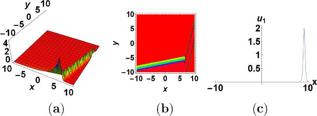
Figure 1. The superposition wave solution u1 for the expression ( |
Based on the dynamic characteristics presented in the above graphs, we find that the velocity at the top of the wave is consistent with the velocity at the bottom of the wave. Therefore, the solitary wave discussed above can propagate without changing its shape. The parameters are related to the pulse width. Solitons remain unchanged in shape during their motion and remain undamaged. If they are applied in the field of communication, we can achieve the goal of controlling pulse width by changing the value of parameters.
Secondary superposition, from (61 ) and (63 ), we can assume that 65 ) into (64 ) we get the. First, select the following parameters
$\begin{eqnarray}\begin{array}{rcl}{f}_{0} & = & 1,\\ {f}_{1} & = & 1+h{\,\rm{e}\,}^{1+d+x{a}_{1}+t{a}_{4}-\frac{y\left({a}_{4}-2{a}_{1}^{3}{l}_{3}+{a}_{1}^{3}{l}_{4}+{a}_{1}{l}_{5}\right)}{2{l}_{6}-{l}_{7}}}\\ & & -\frac{z\left({a}_{4}-2{a}_{1}^{3}{l}_{3}+{a}_{1}^{3}{l}_{4}+{a}_{1}{l}_{5}\right)}{2{l}_{6}-{l}_{7}},\\ {f}_{2} & = & {f}_{12}=h{{\rm{e}}}^{{A}_{1}}-k{{\rm{e}}}^{{A}_{2}}+hk\frac{1}{{a}_{1}+{b}_{1}}{{\rm{e}}}^{{A}_{1}+{A}_{2}}{a}_{1}\\ & & -hk\frac{1}{{a}_{1}+{b}_{1}}{{\rm{e}}}^{{A}_{1}+{A}_{2}}{b}_{1},\end{array}\end{eqnarray}$
where h, k, ai, bi, d (i = 1, 2, 3) are constants and fj(x, t, y, z) (j = 0, 1, 2) are the functions of the variables x, y, z and t. In order to facilitate the calculation, the values of and parameters are taken, then ( $\begin{eqnarray}\begin{array}{c}{f}_{1}:{a}_{1}={l}_{6}={l}_{7}={a}_{4}=z=h={l}_{3}=1,d=2,{l}_{4}=-1,{l}_{5}=5\\ {f}_{2}:{a}_{1}=1,d={l}_{6}=-2,{l}_{7}=d={l}_{6}={l}_{7}={a}_{4}=1,h=-7,\\ {l}_{3}=3,{l}_{4}=-1,{l}_{5}=5,{b}_{1}=2,{b}_{4}=6.\end{array}\end{eqnarray}$
We get $\begin{eqnarray}\begin{array}{rcl}{f}_{1} & = & 1+{\rm{e}}^{t+x-3y},{f}_{2}=-7{\rm{e}}^{-2-\frac{41y}{5}}7{\rm{e}}^{7t+3x}\\ & & -2{\rm{e}}^{\frac{1}{5}(5+30t+10x+y)}+{\rm{e}}^{1+t+x+8y}\\ {f}_{12} & = & 7{\rm{e}}^{-2-\frac{56y}{5}}+\frac{7}{2}{\rm{e}}^{8t+4x}\\ & & -\frac{2}{3}{\rm{e}}^{1+7t+3x+\frac{y}{5}}+7{\rm{e}}^{7t+3x+3y}\\ & & -2{\rm{e}}^{1+6t+2x+\frac{16y}{5}}+{\rm{e}}^{1+t+x+11y}.\end{array}\end{eqnarray}$
We get the three-dimensional map, a contour map of the superposition wave solution obtained from the expressions (2) by selecting the parameters, which are shown in figure 2. It can be seen that there are two bell waves in the graph of the superposition wave solution. The two solitons in figure 2 are of the same type, and in the same direction, as the time variable t increases, the two solitons maintain parallel motion.
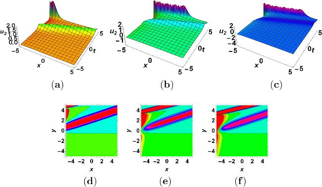
Figure 2. The superposition wave solution u2 for the expression (68), (a) is u2 with t = 8, (a) is u2 with t = 6.4, (c) is u2 with t = 5.95. |
7.2. Double soliton superposition solution
In order to obtain the superposition solution of the equation two solitons, the assumption is made 40 ), when we select the parameters d = l6 = − 2, h = − 7, l3 = 3, l4 =− 1, l5 = 5, b1 = 2, b4 = 6, d = a1 = l6 = l7 = a4 = 1. We obtain
$\begin{eqnarray}\begin{array}{rcl}{f}_{0} & = & 1,\\ {f}_{1} & = & {f}_{2}=h{{\rm{e}}}^{{A}_{1}}-k{{\rm{e}}}^{{A}_{2}}+hk{a}_{1}\frac{1}{{a}_{1}+{b}_{1}}{{\rm{e}}}^{{A}_{1}+{A}_{2}}\\ & & -hk\frac{1}{{a}_{1}+{b}_{1}}{{\rm{e}}}^{{A}_{1}+{A}_{2}}{b}_{1},\\ {A}_{1} & = & 1+x{a}_{1}+\frac{{A}_{3}}{2{l}_{6}-{l}_{7}},{A}_{2}=1+x{b}_{1}+\frac{{A}_{4}}{2{l}_{6}-{l}_{7}}.\\ {A}_{3} & = & -y{a}_{4}-z{a}_{4}+2y{a}_{1}^{3}{l}_{3}+2z{a}_{1}^{3}{l}_{3}-y{a}_{1}^{3}{l}_{4}-z{a}_{1}^{3}{l}_{4}\\ & & -y{a}_{1}{l}_{5}-z{a}_{1}{l}_{5}+2d{l}_{6}+2t{a}_{4}{l}_{6}-d{l}_{7}-t{a}_{4}{l}_{7}\\ {A}_{4} & = & -y{b}_{4}-z{b}_{4}+2y{b}_{1}^{3}{l}_{3}+2z{b}_{1}^{3}{l}_{3}-y{b}_{1}^{3}{l}_{4}-z{b}_{1}^{3}{l}_{4}\\ & & -y{b}_{1}{l}_{5}-z{b}_{1}{l}_{5}+2d{l}_{6}+2t{b}_{4}{l}_{6}-d{l}_{7}-t{b}_{4}{l}_{7}\end{array}\end{eqnarray}$
Then, substitute expressions (67) into formula ( $\begin{eqnarray}\begin{array}{rcl}{f}_{12} & = & -7{{\rm{e}}}^{-2-\frac{41y}{5}-\frac{41z}{5}}\left(\frac{7}{3}{{\rm{e}}}^{7t+3x}\right.\\ & & \left.+{{\rm{e}}}^{1+t+8y+8z}-{{\rm{e}}}^{2x+\frac{1}{5}(5+30t+y+z)}\right).\end{array}\end{eqnarray}$
In figure 3, we can see that the image of the superposition solution moves with the change of t, and the shape remains unchanged, the velocity depends on the shape of the wave and the depth of the water surface, the two waves meet and remain the same shape, which happens to be an important characteristic of solitary waves.
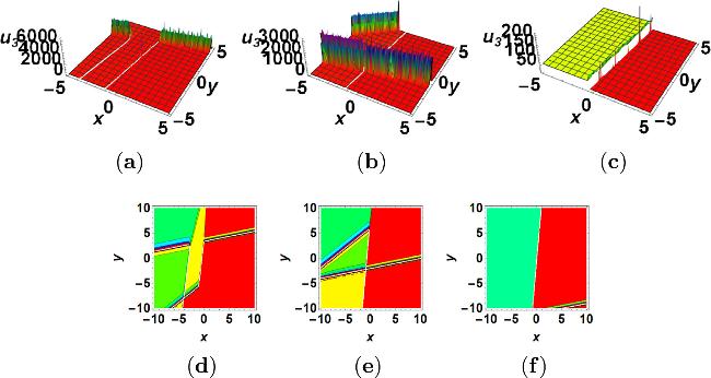
Figure 3. The superposition wave solution u3 for the expression (68). The parameters are (a)(d) t = − 3.4, (b)(e) t = 2, (c)(f) t = 11. |
7.3. Breath soliton superposition solution
Suppose there is a respirator solution of the equation in the form of 71 ) into formula (35 ) to get 70 ) into (69 ), and then substitute the new (69 ) obtained into (40 ). Thus we can obtain a3 = a4 = b1 = a7=b4 = b5 = l6=h3 = l4 = 2, b2=k1 = k2 = a5=a1 = h1 = h2=z = l5 = b6 = 1, k3 = b3 = l3 =− 1, b7 = − 2, b8 = 2, l7 = 3.
$\begin{eqnarray}\begin{array}{rcl}{f}_{0} & = & 1\\ {f}_{1} & = & {k}_{1}{\rm{e}\,}^{x{a}_{1}+y{a}_{2}+z{a}_{3}+t{a}_{4}}+{k}_{1}{\,\rm{e}}^{-\left(x{a}_{1}+y{a}_{2}+z{a}_{3}+t{a}_{4}\right)}\\ & & +{k}_{3}\cos (x{a}_{5}+y{a}_{6}+t{a}_{8}+{a}_{7}z),\\ {f}_{2} & = & {h}_{1}{\rm{e}\,}^{x{b}_{1}+y{b}_{2}+z{b}_{3}+t{b}_{4}}+{h}_{1}{\,\rm{e}}^{-\left(x{b}_{1}+y{b}_{2}+z{b}_{3}+t{b}_{4}\right)}\\ & & +{h}_{3}\cos (x{b}_{5}+y{b}_{6}+t{b}_{8}+{b}_{7}z),\end{array}\end{eqnarray}$
where hi, ki, ai, bi (i = 1, 2, 3, …, 8) are constants, and fj(x, y, z, t) are the functions of the variables x, y, z and t. Substitute expressions ( $\begin{eqnarray}\begin{array}{rcl}{a}_{8} & = & \frac{1}{2}(-{a}_{5}^{3}{l}_{3}-{a}_{5}^{3}{l}_{4}-2{a}_{5}{l}_{5}-{a}_{6}{l}_{6}-{a}_{6}{l}_{7}),\\ {a}_{2} & = & {a}_{3}=\frac{-2{a}_{4}+{a}_{1}^{3}{l}_{3}+{a}_{1}^{3}{l}_{4}-2{a}_{1}{l}_{5}}{{\,}_{6}+{l}_{7}},{a}_{7}={a}_{6}.\end{array}\end{eqnarray}$
Substitute (The three-dimensional diagram and contour plot of the superposition solution of the breathing solution are shown in figure 4, and the unused t is selected to obtain the image of the superposition solution as a function of t. The superposition solution is obtained by the collision of two breathing waves, and the shape of the wave does not change with the change of t, which is stable.
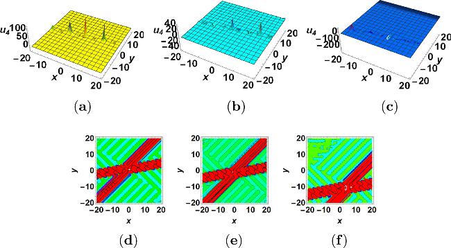
Figure 4. The superposition wave solution u3 for expression ( |
The quadratic superposition of the respiratory wave solution of the equation, in the same way we assume 71 ) into (40 ), for the convenience of calculation, we select the suitable parameters before calculating 72 ) into (71 ), we can get
$\begin{eqnarray}\begin{array}{rcl}{f}_{0} & = & 1,\\ {f}_{1} & = & {\rm{e}\,}^{-x{a}_{1}-t{a}_{4}-{B}_{1}}{k}_{1}+{\,\rm{e}}^{x{a}_{1}+t{a}_{4}+{B}_{1}}{k}_{1}\\ & & +\cos (x{a}_{5}+y{a}_{6}+z{a}_{6}+\frac{t}{2}{B}_{3}){k}_{3},\\ {f}_{2} & = & {\rm{e}\,}^{-x{b}_{1}-t{b}_{4}-{B}_{2}}{h}_{1}+{\,\rm{e}}^{x{b}_{1}+t{b}_{4}+{B}_{2}}{h}_{1}\\ & & +\cos (x{b}_{5}+y{b}_{6}+z{b}_{6}+\frac{t}{2}{B}_{4}){h}_{3},\\ {B}_{1} & = & \frac{y(-2{a}_{4}+{a}_{1}^{3}{l}_{3}+{a}_{1}^{3}{l}_{4}-2{a}_{1}{l}_{5})}{{l}_{6}+{l}_{7}}\\ & & -\frac{z(-2{a}_{4}+{a}_{1}^{3}{l}_{3}+{a}_{1}^{3}{l}_{4}-2{a}_{1}{l}_{5})}{{l}_{6}+{l}_{7}},\\ {B}_{2} & = & \frac{y(-2{b}_{4}+{b}_{1}^{3}{l}_{3}+{b}_{1}^{3}{l}_{4}-2{b}_{1}{l}_{5})}{{l}_{6}+{l}_{7}}\\ & & -\frac{z(-2{b}_{4}+{b}_{1}^{3}{l}_{3}+{b}_{1}^{3}{l}_{4}-2{b}_{1}{l}_{5})}{{l}_{6}+{l}_{7}},\\ {B}_{3} & = & -{a}_{5}^{3}{l}_{3}-{a}_{5}^{3}{l}_{4}-2{a}_{5}{l}_{5}-{a}_{6}{l}_{6}-{a}_{6}{l}_{7},\\ {B}_{4} & = & -{b}_{5}^{3}{l}_{3}-{b}_{5}^{3}{l}_{4}-2{b}_{5}{l}_{5}-{b}_{6}{l}_{6}-{b}_{6}{l}_{7}.\end{array}\end{eqnarray}$
Taking ( $\begin{eqnarray}\begin{array}{rcl}{a}_{1} & = & {a}_{5}={a}_{8}={k}_{1}={k}_{2}={b}_{6}={l}_{5}={h}_{1}={h}_{2}=z=1,{l}_{7}=3,\\ & & {a}_{6}={k}_{3}={l}_{3}=-1,\\ {b}_{1} & = & {a}_{4}={a}_{7}={b}_{4}={b}_{5}={b}_{8}={l}_{4}={l}_{6}={h}_{3}=2,{b}_{7}=-2.\end{array}\end{eqnarray}$
Taking ( $\begin{eqnarray}\begin{array}{rcl}{f}_{0} & = & 1,\\ {f}_{1} & = & {\rm{e}\,}^{-1+2t+x-y}+{\,\rm{e}}^{1-2t-x+y}-\cos (1-t-x+y),\\ {f}_{2} & = & {\rm{e}\,}^{-\frac{3}{5}+t+x-\frac{3y}{5}}+{\,\rm{e}}^{\frac{3}{5}-t-x+\frac{3y}{5}}+2\cos (1-4t+x+y),\\ {f}_{12} & = & {\,\rm{e}\,}^{-1-2t-x-y}(-{\,\rm{e}\,}^{t+\frac{8(1+y)}{5}}+{\,\rm{e}\,}^{3t+\frac{2}{5}(1+5x+y)})\sin (1-t-x+y)\\ & & +2(-{\,\rm{e}\,}^{3t+x+\frac{3(1+y)}{5}}x+{\,\rm{e}\,}^{t+x+\frac{7(1+y)}{5}}x\\ & & +(-{\rm{e}\,}^{4t+2x}+{\,\rm{e}}^{2+2y})\\ & & \times \sin (1-4t+x+y)+{\,\rm{e}\,}^{1+2t+x+y}x\sin (2-5t+2y)).\end{array}\end{eqnarray}$
We can get the three-dimensional map, contour map and line plots. When we perform a quadratic superposition of the breathing solution, we find that the resulting superposition solution is periodic and the width between waves is the same, which means that the solution contains trigonometric and exponential functions.
7.4. Rogue waves superposition solution
In order to obtain the superposition solution of the rogue wave solution of the equation, we assume that 76 ) into formula (35 ) to get 75 ) into (74 ), then taking (74 ) into (40 ), we can obtain f12. When we take the suitable parameters
$\begin{eqnarray}\begin{array}{rcl}{f}_{0} & = & 1,\\ {f}_{1} & = & {(x{a}_{1}+y{a}_{2}+z{a}_{3}+t{a}_{4})}^{2}+{k}_{1}{(x{a}_{5}+y{a}_{6}+z{a}_{7}+t{a}_{8})}^{2}\\ & & +k\cos ({a}_{9}x+y{a}_{10}+t{a}_{11}+{a}_{12}z),\\ & & \times {f}_{2}={(x{b}_{1}+y{b}_{2}+z{b}_{3}+t{b}_{4})}^{2}+{h}_{1}{(x{b}_{5}+y{b}_{6}+z{b}_{7}+t{b}_{8})}^{2}\\ & & +h\cos ({b}_{9}x+y{b}_{10}+t{b}_{11}+{b}_{12}z).\end{array}\end{eqnarray}$
Substitute expressions ( $\begin{eqnarray}\begin{array}{rcl}{a}_{12} & = & \frac{{tC}}{2(-{a}_{3}{a}_{5}+{a}_{1}{a}_{7})},{a}_{6}={a}_{7},{a}_{10}={a}_{11},{a}_{2}={a}_{3},\\ {l}_{5} & = & \frac{-{a}_{4}{a}_{7}+{a}_{3}{a}_{8}}{-{a}_{3}{a}_{5}+{a}_{1}{a}_{7}},{l}_{7}=\frac{2{a}_{4}{a}_{5}-2{a}_{1}{a}_{8}+{a}_{3}{a}_{5}{l}_{6}-{a}_{1}{a}_{7}{l}_{6}}{-{a}_{3}{a}_{5}+{a}_{1}{a}_{7}},\\ C & = & 2{a}_{4}{a}_{7}{a}_{9}-2{a}_{3}{a}_{8}{a}_{9}-2{a}_{4}{a}_{5}{a}_{11}+2{a}_{1}{a}_{8}{a}_{11}+{a}_{3}{a}_{5}{a}_{9}^{3}{l}_{3}\\ & & -{a}_{1}{a}_{7}{a}_{9}^{3}{l}_{3}+{a}_{3}{a}_{5}{a}_{9}^{3}{l}_{4}-{a}_{1}{a}_{7}{a}_{9}^{3}{l}_{4}.\end{array}\end{eqnarray}$
Taking ( $\begin{eqnarray}\begin{array}{c}{a}_{1}={b}_{1}={a}_{3}={a}_{5}={a}_{8}={b}_{2}={k}_{1}={b}_{4}={b}_{6}={b}_{8}={l}_{3}={l}_{4}\\ =\,{l}_{5}={l}_{6}={l}_{7}=z={a}_{9}={a}_{10}={b}_{9}={b}_{11}=k=1\\ {a}_{2}={a}_{6}={b}_{3}={b}_{5}=-1,{a}_{4}={a}_{7}=2,{a}_{11}=3,{b}_{7}=-2,\end{array}\end{eqnarray}$
we can obtain $\begin{eqnarray}\begin{array}{c}{\,f}_{12}=-({(-1+t+3x-y)}^{2}+{(1+t+x+y)}^{2}+\cos (3+t+x+3y))\\ (2(-1+t+x-y)+2(1+t+x+y)-\sin (2+x+2y))\\ +\,({(-1+t+x-y)}^{2}+{(1+t+x+y)}^{2}+\cos (2+x+2y))\\ (6(-1+t+3x-y)+2(1+t+x+y)-\sin (3+t+x+3y)).\end{array}\end{eqnarray}$
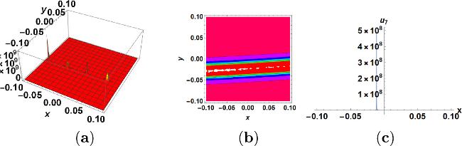
By choosing different values of t, the superposition solution of the equation and the relationship between the solution and t can be obtained. From figure 6, we can see that the superimposed wave consists of two waves and they collide with the transformation of t, but the overall shape does not change.
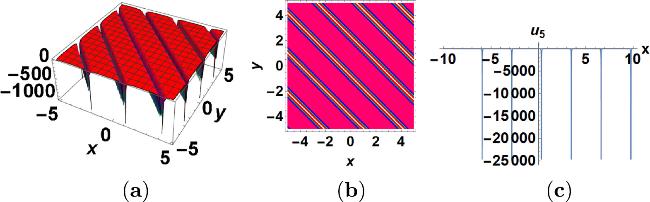
Figure 5. The superposition wave solution u5 for the expression ( |
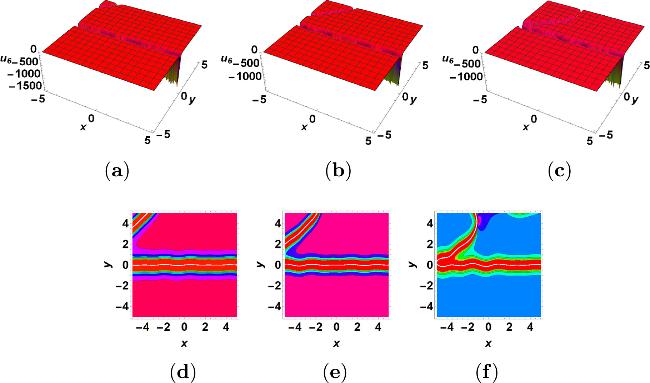
Figure 6. The superposition wave solution u3 for the expression ( |
The quadratic superposition of the respiratory wave solution of the equation, in the same way we assume
$\begin{eqnarray}\begin{array}{rcl}{f}_{0} & = & 1,\\ {f}_{1} & = & {\left(-1+t+3x-y\right)}^{2}+{\left(1+t+x+y\right)}^{2}\\ & & +\cos (3+t+x+3y),\\ {f}_{2} & = & -[{(1+t+x-y)}^{2}+{(1+t+x+y)}^{2}\\ & & +\cos (3+t+x+3y)]\\ & & \times [2(-1+t+x-y)+2(1+t+x+y)\\ & & -\sin (2+x+2y)]\\ & & +[{(-1+t+x-y)}^{2}+{(1+t+x+y)}^{2}\\ & & +\cos (2+x+2y)]\\ & & \times [6(-1+t+3x-y)+2(1+t+x+y)\\ & & -\sin (3+t+x+3y)].\end{array}\end{eqnarray}$
Then by taking (78 ) into (40 ), we can get the three-dimensional map, contour map and line plots.
As can be seen from the diagram, the rouge superposition wave solution consists of multiple strange waves, which do not collide and are located in the same straight line. It can also be seen that the maximum value of the superimposed wave solution is from figure 5(c).
8. Conclusion
In this paper, we investigate a (3+1)-dimensional generalized CBS equation. Initially, employing the symbolic calculation system and Bell polynomial approach, we derive the bilinear form of the equation, bilinear Bäcklund transformation, Lax pair, and infinite conservation laws. This derivation confirms the complete integrability of the CBS equation in the context of the Lax pair.
Furthermore, utilizing the derived bilinear Bäcklund transformation, we construct a nonlinear superposition formula for the CBS equation. Based on this formula, we generate infinite superposition soliton solutions. Additionally, leveraging the bilinear equation, we obtain infinite superposition solutions encompassing various types of functions. The graphical representations of these solutions, as depicted in figures 1–7, illustrate distinct dynamic characteristics. Specifically, figures 1–3 showcase superposition solutions formed by an exponential function, exhibiting a continuous V-shape with increasing wave diversity as the number of superposed exponential functions rises. Figures 4 and 5 depict waves combining exponential and trigonometric functions, revealing periodic respiratory solutions. Figures 6 and 7 highlight the morphological features of primary and quadratic superposition wave solutions of unusual wave forms, demonstrating the properties and characteristics of different function types and their mixtures.
Figure 7. The superposition wave solution u7 for the expression ( |
Notably, this study not only extracts numerous properties through the Bell polynomial method but also formulates a nonlinear superposition formula for the CBS equation, enabling the derivation of infinite superposition solutions. Moreover, we construct linear infinite superposition solutions based on the bilinear form of the CBS equation, enriching the array of exact solutions. This research presents the first comprehensive examination of the CBS equation. Future work may explore the construction of interaction solutions among infinite superposition solutions of other function types to further expand the range of precise and insightful solutions.
Credit authors statement
XZ wrote the manuscript, analyzed the data, and wrote the code for the model. TB initiated the concept of the study, developed the model, and acted as the corresponding author.
Funding
The authors gratefully acknowledge the support of the Natural Science Foundation of Inner Mongolia Autonomous Region (Grant No. 2024MS01003), the First-Class Disciplines Project, Inner Mongolia Autonomous Region, China (Grant Nos. YLXKZX-NSD-001 and YLXKZX-NSD-009) and the Program for Innovative Research Team in Universities of Inner Mongolia Autonomous Region (Grant No. NMGIRT2414).
Appendix
$\begin{eqnarray}\begin{array}{rcl} & & {D}_{x}({D}_{x}^{3}a\cdot b)\cdot ab\\ & = & {D}_{x}^{3}({D}_{x}a\cdot b)\cdot ab+3{D}_{x}({D}_{x}^{2}a\cdot b)\cdot ({D}_{x}a\cdot b),\end{array}\end{eqnarray}$
$\begin{eqnarray}\begin{array}{rcl} & & ({D}_{x}a\cdot b)cd-ab{D}_{x}c\cdot d\\ & = & {D}_{x}ad\cdot cb,\end{array}\end{eqnarray}$
$\begin{eqnarray}\begin{array}{l}({D}_{x}^{5}a\cdot b)\cdot cd-ab{D}_{x}^{5}c\cdot d=\frac{5}{16}{D}_{x}[ad\cdot ({D}_{x}^{4}c\cdot d)+({D}_{x}^{4}a\cdot d)\cdot cd]\\ \quad +\,4({D}_{x}a\cdot d),\\ ({D}_{x}^{3}c\cdot b)+4({D}_{x}^{3}a\cdot d)\cdot ({D}_{x}c\cdot b)+6({D}_{x}^{2}a\cdot d)\cdot ({D}_{x}^{2}c\cdot b)]\\ \quad +\,\frac{5}{8}{D}_{x}^{3}[ad\cdot ({D}_{x}^{2}c\cdot b)\\ +\,2({D}_{x}a\cdot d)({D}_{x}c\cdot b)]+({D}_{x}^{2}a\cdot d)\cdot cb]+\frac{1}{16}{D}_{x}^{5}ad\cdot cb,\end{array}\end{eqnarray}$
$\begin{eqnarray}\begin{array}{l}9{D}_{x}({D}_{x}^{5}a\cdot b)\cdot ab+{D}_{x}^{5}({D}_{x}a\cdot b)\cdot ab+5{D}_{x}({D}_{x}a\cdot b)\cdot ({D}_{x}^{4}a\cdot b)-30{D}_{x}({D}_{x}^{3}a\cdot b),\\ ({D}_{x}^{2}a\cdot b)+10{D}_{x}^{3}({D}_{x}a\cdot b)+10{D}_{x}^{3}({D}_{x}a\cdot b)\cdot ({D}_{x}^{2}a\cdot b)-10{D}_{x}^{3}({D}_{x}^{3}a\cdot b)\cdot ab=0,\end{array}\end{eqnarray}$
$\begin{eqnarray}\begin{array}{l}({D}_{x}^{3}a\cdot b)c-({D}_{x}^{3}a\cdot c)b\\ =-3{a}_{xx}{D}_{x}b\cdot c+3{a}_{x}{({D}_{x}b\cdot c)}_{x}-\frac{1}{4}a[{D}_{x}^{3}b\cdot c+3{({D}_{x}b\cdot c)}_{xx}],\end{array}\end{eqnarray}$
$\begin{eqnarray}\begin{array}{l}{({D}_{x}^{3}a\cdot b)}_{x}c-{({D}_{x}^{3}a\cdot c)}_{x}b=-2{a}_{xxx}{D}_{x}b\cdot c\\ +\frac{1}{2}{a}_{x}[{D}_{x}^{3}b\cdot c+3{({D}_{x}b\cdot c)}_{xx}]-\frac{1}{2}a[{({D}_{x}^{3}b\cdot c)}_{x}+{({D}_{x}b\cdot c)}_{xx}],\end{array}\end{eqnarray}$
$\begin{eqnarray}({D}_{t}a\cdot b)c-({D}_{t}a\cdot c)b=-a{D}_{t}b\cdot c,\end{eqnarray}$
$\begin{eqnarray}({D}_{x}a\cdot b)cd-ab{D}_{x}c\cdot d={D}_{x}ad\cdot cb,\end{eqnarray}$
$\begin{eqnarray}\begin{array}{l}{({D}_{t}a\cdot b)}_{x}c-{({D}_{t}a\cdot c)}_{x}b\\ =\,{a}_{t}{D}_{x}b\cdot c+{a}_{x}{D}_{t}b\cdot c-\frac{1}{2}a[{({D}_{x}a\cdot c)}_{t}+{({D}_{t}b\cdot c)}_{x}],\end{array}\end{eqnarray}$
$\begin{eqnarray}\begin{array}{l}({D}_{x}{D}_{t}a\cdot b)c-({D}_{x}{D}_{t}a\cdot c)b\\ =\,-{a}_{x}{D}_{t}b\cdot c-{a}_{t}{D}_{x}b\cdot c+\frac{1}{2}a[{({D}_{x}b\cdot c)}_{t}+{({D}_{t}b\cdot c)}_{x}],\end{array}\end{eqnarray}$
$\begin{eqnarray}\begin{array}{l}{k}_{1}({D}_{x}a\cdot b)c-{k}_{2}({D}_{x}a\cdot c)b\\ =\,({k}_{1}-{k}_{2}){a}_{x}bc-\frac{1}{2}a[({k}_{1}+{k}_{2}){D}_{x}b\cdot c+({k}_{1}-{k}_{2}){(bc)}_{x}],\end{array}\end{eqnarray}$
$\begin{eqnarray}\begin{array}{l}{A}_{1}=1+x{a}_{1}\\ +\,\frac{-y{a}_{4}-z{a}_{4}+2y{a}_{1}^{3}{l}_{3}+2z{a}_{1}^{3}{l}_{3}-y{a}_{1}^{3}{l}_{4}-z{a}_{1}^{3}{l}_{4}-y{a}_{1}{l}_{5}-z{a}_{1}{l}_{5}+2d{l}_{6}+2t{a}_{4}{l}_{6}-d{l}_{7}-t{a}_{4}{l}_{7}}{2{l}_{6}-{l}_{7}},\\ {A}_{2}=1+x{b}_{1}\\ +\,\frac{-y{b}_{4}-z{b}_{4}+2y{b}_{1}^{3}{l}_{3}+2z{b}_{1}^{3}{l}_{3}-y{b}_{1}^{3}{l}_{4}-z{b}_{1}^{3}{l}_{4}-y{b}_{1}{l}_{5}-z{b}_{1}{l}_{5}+2d{l}_{6}+2t{b}_{4}{l}_{6}-d{l}_{7}-t{b}_{4}{l}_{7}}{2{l}_{6}-{l}_{7}}.\end{array}\end{eqnarray}$