


1. Introduction
Distinguishing between two quantum statistical objects is a central task in quantum information theory. So mathematical methods underlying distinguishability have been studied for a long time [1–3] and are now highly developed under the general framework of quantum hypothesis testing [4, 5]. Briefly speaking, the hypothesis testing theory means that, with sufficient statistical evidence, one can determine which hypothesis should be rejected in favor of the other and if the null hypothesis is accepted, one can form alternative hypotheses to test against the null hypothesis in future experiments. Quantum hypothesis testing is an important topic in the sense that it has wide applications to quantum communication [6, 7], and quantum computation [8].
The most basic setting is that of state discrimination where we are given a quantum state that is either in the state ρ or in the state σ. The goal of the distinguisher, who does not know a priori which state was prepared, is to determine the identity of the unknown state. Here we consider the independent and identically distributed (IID) case: given n quantum systems in the state ρ⨂n or σ⨂n, the task is to apply a binary measurement {Qn, I⨂n − Qn} with 0 ≤ Qn ≤ I⨂n, to determine which state one possesses. Then two kinds of error probabilities occur:
$\begin{eqnarray}{\alpha }_{n}({Q}_{n})={\rm{Tr}}\{({I}^{\otimes n}-{Q}_{n}){\rho }^{\otimes n}\},\,\,({\rm{t}}{\rm{y}}{\rm{p}}{\rm{e}}I)\end{eqnarray}$
$\begin{eqnarray}{\beta }_{n}({Q}_{n})={\rm{Tr}}\{{Q}_{n}{\sigma }^{\otimes n}\},\,\,\,({\rm{t}}{\rm{y}}{\rm{p}}{\rm{e}}II).\end{eqnarray}$
When a constant threshold ϵ is imposed on the type I error, the optimal type II error is given by $\begin{eqnarray}{\beta }_{\varepsilon }(\rho \parallel \sigma )=\min \{\beta (Q):0\,\leqslant \,Q\,\leqslant \,I,\alpha (Q)\,\leqslant \,\varepsilon \}.\end{eqnarray}$
The quantum stein’s lemma states that [4, 5, 9, 10]
$\begin{eqnarray}\begin{array}{l}\mathop{\mathrm{lim}}\limits_{n\to \infty }\frac{1}{n}{D}_{H}^{\varepsilon }({\rho }^{\displaystyle \otimes n}\parallel {\sigma }^{\displaystyle \otimes n})\\ \quad =\mathop{\mathrm{lim}}\limits_{n\to \infty }-\frac{1}{n}\mathrm{log}{\beta }_{\varepsilon }({\rho }^{\displaystyle \otimes }\parallel {\sigma }^{\displaystyle \otimes })=D(\rho \parallel \sigma ),\end{array}\end{eqnarray}$
where ${D}_{H}^{\varepsilon }(\rho \parallel \sigma )$ = $-\mathrm{log}\inf \{{\rm{Tr}}(Q\sigma ):0\,\leqslant \,Q\,\leqslant \,I,{\rm{Tr}}(Q\rho )\geqslant 1-\varepsilon \}$ denotes the quantum hypothesis testing relative entropy and D(ρ∥σ), the standard quantum relative entropy. It is also remarkable that the quantum stein’s lemma provides a rigorous operational interpretation for the quantum relative entropy.Although research in quantum hypothesis testing has largely focused on quantum states, there are various situations in which quantum channels play the role of the main objects of study. The task of channel discrimination is quite different from that of state discrimination due to its nature as dynamic resources [6, 11–16]. Unlike state discrimination, the dynamic feature of quantum channels raises challenging difficulties in determining the optimal discrimination scheme as we have to handle the additional optimization of the input states and the non-IID structure of the testing states [17]. In addition, we need to consider what role the discrimination strategies play in the quantum channel discrimination. Despite inherent mathematical links between the channel and state discrimination problems, the discrimination of channels is more complicated, due to the additional degrees of freedom introduced by the adaptive strategies. Several works have been dedicated to study the potential advantages of adaptive strategies over nonadaptive strategies in channel discrimination [18, 19]. It is known that asymptotically the exponential error rate for classical-quantum channel discrimination is not improved by adaptive strategies [11, 16, 20]. However, there indeed exists separation between adaptive and nonadaptive symmetric hypothesis testing exponents for quantum channels, and the concrete example is provided in [20]. For quantum-quantum channels, i.e., channels having quantum input and quantum outputs, it is shown that adaptive strategies provide an advantage in the non-asymptotic regime for discrimination in the symmetric Chernoff setting [18, 21, 22]. Therefore, a deeper understanding and analysis on hypothesis testing of quantum channels is imperative.
It is well known in information theory literature [23, 24] that the error probability decreases exponentially fast in the number of samples provided, that is, extra samples are helpful for decreasing the error probability when trying to determine the unknown objects. So it is desirable to consider the natural problem that given a constant upper bound on the desired error probability, how the distinguisher determines the value of x with as few samples as possible (minimize n) while meeting the error probability constraint. This notion is often called sampling complexity in the literature of algorithms and machine learning [25, 26]. It is useful because it indicates how long one needs to wait in order to make a decision with a desired performance [27].
In this paper, we systematically study the sampling complexity of channel discrimination under the framework of quantum hypothesis testing. Here, we take two discrimination strategies into consideration. The product strategy for n uses of the channel consists of feeding an input state into the n-fold tensor product channel. The adaptive strategy refers to the way of sending the initial state to the given channel followed by applying an update channel. We provide the lower and upper bound on the sampling complexity with respect to the symmetric, asymmetric and error exponent settings. These bounds are characterized by various channel divergences defined below. Two particular examples are considered. We find the amortized channel divergence collapses into generalized channel divergence for the classical-quantum channel, which indicates that in such a case, the lower and upper bounds appeared in the main theorems for two different strategies are completely equal. Thus, the adaptive strategy can not lead to an advantage to the problem of determining the sampling complexity for classical-quantum channels. For generalized amplitude damping channels, the numerical simulation shows that there is always a gap between amortized channel divergence and generalized channel divergence. That is to say, the adaptive strategy can bring advantages over the product strategy in the task of determining the sampling complexity for generalized amplitude damping channels. This partially clarifies the long-standing question of the usefulness of adaptive strategies in quantum channel discrimination protocols.
2. Preliminaries
2.1. Basic notation
Throughout, we denote the finite dimensional Hilbert space by HA, HB corresponding to physical system A, B. Quantum states of system A are denoted by ${\rho }_{A}\in { \mathcal S }(A)$. A quantum channel ${{ \mathcal N }}_{A\to B}$ is a completely positive (CP) and trace-preserving (TP) linear map from operators acting on HA to operators acting on HB. Let Θ denote a quantum superchannel that takes quantum channel ${{ \mathcal N }}_{A\to B}$ to ${{ \mathcal M }}_{C\to D}$. Then, for any quantum superchannel Θ, it can be physically realized as follows [28]:
$\begin{eqnarray}\begin{array}{l}{{ \mathcal M }}_{C\to D}={\rm{\Theta }}({{ \mathcal N }}_{A\to B})\\ \quad ={{ \mathcal V }}_{BR\to D}\circ ({{ \mathcal N }}_{A\to B}\displaystyle \otimes {{ \mathcal I }}_{R})\circ {{ \mathcal U }}_{C\to AR},\end{array}\end{eqnarray}$
where ${{ \mathcal U }}_{C\to AR}$ is a pre-processing channel, system E corresponds to environmental system, and ${{ \mathcal V }}_{BR\to D}$ is a post-processing channel.Let ρ and σ be two quantum states. The quantum relative entropy is defined as:
$\begin{eqnarray}D(\rho \parallel \sigma )={\rm{Tr}}(\rho (\mathrm{log}\rho -\mathrm{log}\sigma )),\end{eqnarray}$
where ${\rm{Tr}}$ denotes the trace and ${\rm{log}}$ is the logarithm with base 2 throughout the paper. The Petz–Rényi divergence is defined for α ∈ (0, 1) ∪ (1, ∞) as [29, 30]: $\begin{eqnarray}{D}_{\alpha }(\rho \parallel \sigma )=\frac{1}{\alpha -1}\mathrm{log}{\rm{Tr}}[{\rho }^{\alpha }{\sigma }^{1-\alpha }].\end{eqnarray}$
Recently, the Sandwiched Rényi relative entropy was introduced in [31]: $\begin{eqnarray}{\tilde{D}}_{\alpha }(\rho \parallel \sigma )=\frac{1}{\alpha -1}\mathrm{log}{\rm{Tr}}\{{\left({\sigma }^{\frac{1-\alpha }{2\alpha }}\rho {\sigma }^{\frac{1-\alpha }{2\alpha }}\right)}^{\alpha }\},\end{eqnarray}$
when the support of ρ is contained in the support of σ and it is equal to + ∞ otherwise. It is known [32] that in the limit α → 1 and α → + ∞, $\begin{eqnarray}\mathop{\mathrm{lim}}\limits_{\alpha \to 1}{\tilde{D}}_{\alpha }(\rho \parallel \sigma )=\mathop{\mathrm{lim}}\limits_{\alpha \to 1}{D}_{\alpha }(\rho \parallel \sigma )=D(\rho \parallel \sigma ),\end{eqnarray}$
and $\begin{eqnarray}\mathop{\mathrm{lim}}\limits_{\alpha \to +\infty }{\tilde{D}}_{\alpha }(\rho \parallel \sigma )={D}_{\max }(\rho \parallel \sigma )=\inf \{\lambda :\rho \,\leqslant \,{2}^{\lambda }\sigma \}.\end{eqnarray}$
In particular, Dα(ρ∥σ) and ${\tilde{D}}_{\alpha }(\rho \parallel \sigma )$ were shown to obey the desirable monotonicity inequality for all α ∈ [0, 1) ∪ (1, + 2) and $\alpha \in [\frac{1}{2},1)\cup (1,+\infty )$ [33], respectively. The Uhlmann, fidelity between the two quantum states ρ and σ is defined as $F(\rho ,\sigma )=\parallel \sqrt{\rho }\sqrt{\sigma }{\parallel }_{1}$, where ∥ · ∥1 denotes the trace norm. Obviously, we have that ${\tilde{D}}_{\frac{1}{2}}(\rho \parallel \sigma )=-2\mathrm{log}F(\rho ,\sigma )$.
The divergence between the quantum states can be naturally extended to quantum channels. The main idea is to quantify the maximum divergence between the outputs from the channels.
Definition 1. (Generalized channel divergence) Given quantum channels${{ \mathcal N }}_{A\to B}$ and${{ \mathcal M }}_{A\to B}$, we define the generalized channel divergence induced by state divergence D as [34]
$\begin{eqnarray}\begin{array}{l}{\boldsymbol{D}}({ \mathcal N }\parallel { \mathcal M })\\ \quad =\,{{\rm{\sup }}}_{{\rho }_{RA}\in { \mathcal S }(RA)}D({{ \mathcal N }}_{A\to B}({\rho }_{RA})\parallel {{ \mathcal M }}_{A\to B}({\rho }_{RA})).\end{array}\end{eqnarray}$
Note that as a consequence of purification, data processing, and the Schmidt decomposition, it follows that the supremum can be restricted to be with respect to pure states.
In order to explore the largest distinguishability that can be realized between the channels, the amortized channel divergence is defined as follows.
Definition 2. (Amortized channel divergence) Given quantum channels${{ \mathcal N }}_{A\to B}$ and ${{ \mathcal M }}_{A\to B}$, we define the amortized channel divergence induced by state divergence D as [16]
$\begin{eqnarray}\begin{array}{l}{{\boldsymbol{D}}}^{{ \mathcal A }}({ \mathcal N }\parallel { \mathcal M })\\ \quad =\,{{\rm{\sup }}}_{{\rho }_{RA},{\sigma }_{RA}\in { \mathcal S }(RA)}[D({{ \mathcal N }}_{A\to B}({\rho }_{RA})\parallel {{ \mathcal M }}_{A\to B}({\sigma }_{RA})-D({\rho }_{RA}\parallel {\sigma }_{RA})].\end{array}\end{eqnarray}$
Note that due to the supremum over the input state, the above two quantities are difficult to calculate in general. However, for specific cases, we can evaluate them numerically or via semi-definite program (SDP). When we choose the state divergence as the max-relative entropy, amortized channel divergence collapses into generalized channel divergence. Then ${{\boldsymbol{D}}}_{\max }^{{ \mathcal A }}({ \mathcal N }\parallel { \mathcal M })$=${{\boldsymbol{D}}}_{\max }({ \mathcal N }\parallel { \mathcal M })={{\boldsymbol{D}}}_{\max }({ \mathcal N }({{\rm{\Phi }}}_{RA})\parallel { \mathcal M }({{\rm{\Phi }}}_{RA}))$ with ΦRA being the maximal entanglement state, which is a SDP and therefore efficiently computable [16]. Another extreme case [6] is when both channels are replacer channels, general divergences are equal to the corresponding divergences of the two states. Similarly, based on the fidelity of the quantum state, we can define the fidelity of the two quantum channels ${ \mathcal N }$ and ${ \mathcal M }$ as follows.
Definition 3. (Fidelity of channel) Given quantum channels ${{ \mathcal N }}_{A\to B}$ and ${{ \mathcal M }}_{A\to B}$, we define the fidelity of channel induced by state fidelity as
$\begin{eqnarray}\begin{array}{l}{\boldsymbol{F}}({ \mathcal N }\parallel { \mathcal M })\\ \quad =\mathop{\inf }\limits_{{\rho }_{RA}\in { \mathcal S }(RA)}F({{ \mathcal N }}_{A\to B}({\rho }_{RA}),{{ \mathcal M }}_{A\to B}({\rho }_{RA})).\end{array}\end{eqnarray}$
The idea behind the fidelity of the quantum channel is to allow for the arbitrary input state to be used to reduce the degree of approximation between the two channels. Intuitively, the definition quantifies the worst-case behavior of the channels for information preservation. We discuss several basic properties of channel fidelity in appendix A , which may be of independent interest.
2.2. Strategies for quantum channel discrimination
The problem of quantum channel discrimination is made mathematically precise by the following hypothesis testing problems for quantum channels. Given two quantum channels ${{ \mathcal N }}_{A\to B}$ and ${{ \mathcal M }}_{A\to B}$ acting on an input system A and an output system B, there are two fundamental different classes of available strategies as follows [6].
(1) Product strategy: in a product strategy the testing state is created by choosing a sequence of input states φ ∈ S(RA) and sending them to the unknown channel ${ \mathcal G }$ individually. The generated testing state is given by ${{ \mathcal G }}^{\otimes n}({\varphi }^{\otimes })$. The class of all product strategies is denoted as product strategies (PRO).
(2) Adaptive strategy: in an adaptive strategy, we first choose an initial state φn ∈ S(R1A1) and send it to one copy of the channel ${ \mathcal G }$ followed by applying an update channel ${{ \mathcal P }}_{1}$. After this, we apply another copy of the channel ${ \mathcal G }$ and then an update channel ${{ \mathcal P }}_{2}$. Then, repeat this process n times. We get the final testing state ${ \mathcal G }\circ {{ \mathcal P }}_{n-1}\circ \ldots \circ {{ \mathcal P }}_{2}\circ { \mathcal G }\circ {{ \mathcal P }}_{1}\circ { \mathcal G }({\varphi }_{n})$ with ${{ \mathcal P }}_{i}\in CPTP({R}_{i}{B}_{i}\to {R}_{i+1}{A}_{i})$. The class of all adaptive strategies is denoted as adaptive strategies (ADP). For more details about adaptive strategy, please refer to the literature [16].
It is clear that PRO ⫅ ADP.
2.3. Setting of quantum hypothesis testing for quantum channel
In this section, we describe the information-theoretic setting for non-asymptotic quantum channel discrimination. For any discrimination strategy Sn, let ρn(Sn) and σn(Sn) denote the output state generated by n uses of the channel depending on whether it is ${ \mathcal N }$ or ${ \mathcal M }$. {Qn, I − Qn} is the measurement part of the strategy. In analogy with (1) and (2), one can define the type I and II error as:
$\begin{eqnarray}{\alpha }_{n}({S}_{n},{Q}_{n})={\rm{Tr}}\{(I-{Q}_{n}){\rho }_{n}({S}_{n})\},\,\,({\rm{t}}{\rm{y}}{\rm{p}}{\rm{e}}I)\end{eqnarray}$
$\begin{eqnarray}{\beta }_{n}({S}_{n},{Q}_{n})={\rm{Tr}}\{{Q}_{n}{\sigma }_{n}({S}_{n})\},\,\,\,({\rm{t}}{\rm{y}}{\rm{p}}{\rm{e}}II).\end{eqnarray}$
The discrimination task is then to decide which hypothesis is true based on the data drawn from an optimal positive operator-valued measure (POVM) which leads to the minimal error probability, as detailed below. The setting of the quantum hypothesis testing can be classified as symmetric and asymmetric depending on whether the two types of decision errors are treated equally.
In the symmetric setting, the two types of errors are treated equally, where the purpose is to minimize the average (Bayesian) of two error probabilities weighted by the prior probabilities [35]. Given a priori probability p that the first channel ${ \mathcal N }$ is selected, the non-asymptotic expected error probability is defined as
$\begin{eqnarray}\begin{array}{l}{p}_{e\{{Q}_{n}\}}(p,{ \mathcal N },{ \mathcal M },n)\\ \quad =\,p{\alpha }_{n}({S}_{n},{Q}_{n})+(1-p){\beta }_{n}({S}_{n},{Q}_{n}).\end{array}\end{eqnarray}$
Then the distinguisher can minimize the error probability expression in (16 ) over all possible measurements. The Helstrom–Holevo theorem [2, 3] states that the optimal error probability of hypothesis testing is as follows:
$\begin{eqnarray}\begin{array}{l}{p}_{e}(p,{ \mathcal N },{ \mathcal M },n)=\mathop{\inf }\limits_{{Q}_{n}}{p}_{e\{{Q}_{n}\}}(p,{ \mathcal N },{ \mathcal M },n)\\ \,=\,\frac{1}{2}(1-\parallel p{\rho }_{n}({S}_{n})-(1-p){\sigma }_{n}({S}_{n}){\parallel }_{1}).\end{array}\end{eqnarray}$
In asymmetric hypothesis testing, the goal of the distinguisher is to minimize the probability of the second kind of error subject to a constraint on the probability of the first kind of error. Given a fix ϵ ∈ (0, 1), we are interested in the following non-asymptotic optimization problem:
$\begin{eqnarray}\begin{array}{l}\zeta (\varepsilon ,{ \mathcal N },{ \mathcal M },n)\\ \quad =\mathop{\inf }\limits_{{Q}_{n}}\{{\beta }_{n}({S}_{n},{Q}_{n})| {\alpha }_{n}({S}_{n},{Q}_{n})\,\leqslant \,\varepsilon \}.\end{array}\end{eqnarray}$
As a refinement of asymmetric hypothesis testing, the error exponent studies that the type II error probability is constrained to decrease exponentially with exponent r > 0. We are then concerned with the error exponent behavior of the type I error under this constraint. This is defined as the non-asymptotic quantity
$\begin{eqnarray}\begin{array}{l}\xi (r,{ \mathcal N },{ \mathcal M },n)\\ \quad =\,\mathop{\inf }\limits_{{Q}_{n}}\{{\alpha }_{n}({S}_{n},{Q}_{n})| {\beta }_{n}({S}_{n},{Q}_{n})\,\leqslant \,{2}^{-rn}\}.\end{array}\end{eqnarray}$
3. Sampling complexity for quantum channel hypothesis testing
3.1. Definitions of sampling complexity
Note that the above quantities (17 )–19 ) are somewhat different from the traditional definitions in the literature [35–37], where they are called Chernoff setting, Stein setting and Hoeffding setting, respectively. Here we are no longer interested in the asymptotic formulas of these quantities. The goal of this paper is to determine the minimum value of n (i.e., minimum number of samples) needed to meet a fixed error probability constraint. These formulations of the hypothesis testing problem are more consistent with the notion of the runtime of a probabilistic or quantum algorithm, for which one typically finds that the runtime depends on the desired error. Indeed, if there are procedures for preparing the various states involved in a given hypothesis testing problem, with fixed runtimes, then the sampling complexity corresponds to the total amount of time one must wait to prepare n samples to achieve a desired error probability [27].
In this section, we formally introduce the definitions of the sampling complexity of quantum hypothesis testing in the following.
Definition 4. (Sampling complexity of (17)) Given quantum channels ${{ \mathcal N }}_{A\to B}$ and ${{ \mathcal M }}_{A\to B}$ and ϵ ∈ (0, 1), we define the sample complexity induced by (17) as
$\begin{eqnarray}{n}^{* }(\varepsilon ,p,{ \mathcal N },{ \mathcal M },n)=\inf \{n:{p}_{e}(p,{ \mathcal N },{ \mathcal M },n)\,\leqslant \,\varepsilon \}.\end{eqnarray}$
Definition 5. (Sampling complexity of (18)) Given quantum channels ${{ \mathcal N }}_{A\to B}$ and ${{ \mathcal M }}_{A\to B}$ and ϵ, δ ∈ (0, 1), we define the sample complexity induced by (18) as
$\begin{eqnarray}\begin{array}{l}{n}^{* }(\delta ,\varepsilon ,{ \mathcal N },{ \mathcal M },n)\\ \quad =\inf \{n:\zeta (\varepsilon ,{ \mathcal N },{ \mathcal M },n)\,\leqslant \,\delta \}.\end{array}\end{eqnarray}$
Definition 6. (Sampling complexity of (19)) Given quantum channels ${{ \mathcal N }}_{A\to B}$ and ${{ \mathcal M }}_{A\to B}$, ϵ ∈ (0, 1), and r > 0, we define the sample complexity induced by (19) as
$\begin{eqnarray}\begin{array}{l}{n}^{* }(\varepsilon ,r,{ \mathcal N },{ \mathcal M },n)\\ \quad =\inf \{n:\xi (r,{ \mathcal N },{ \mathcal M },n)\,\leqslant \,\varepsilon \}.\end{array}\end{eqnarray}$
Indeed, the definitions of sampling complexity above have more explicit expressions, which can be in favor of proceeding to the development of our main results in the next section.
Remark 1. (Equivalent expressions for sampling complexity) By recalling the quantities defined in the above definitions (20–22), we rewrite the sampling complexity in the following ways:
$\begin{eqnarray}\begin{array}{l}{n}^{* }(\varepsilon ,p,{ \mathcal N },{ \mathcal M },n)\\ \quad =\,\inf \{n:\frac{1}{2}(1-\parallel p{\rho }_{n}({S}_{n})-(1-p){\sigma }_{n}({S}_{n}){\parallel }_{1})\,\leqslant \,\varepsilon \}\\ \quad =\,\inf \{n:\parallel p{\rho }_{n}({S}_{n})-(1-p){\sigma }_{n}({S}_{n}){\parallel }_{1}\geqslant 1-2\varepsilon \}.\end{array}\end{eqnarray}$
$\begin{eqnarray}\begin{array}{l}{n}^{* }(\delta ,\varepsilon ,{ \mathcal N },{ \mathcal M },n)=\mathop{\inf }\limits_{{Q}_{n}}\{n:{\beta }_{n}({S}_{n},{Q}_{n})\\ \quad \,\leqslant \,\delta | {\alpha }_{n}({S}_{n},{Q}_{n})\,\leqslant \,\varepsilon \}.\end{array}\end{eqnarray}$
$\begin{eqnarray}\begin{array}{l}{n}^{* }(\varepsilon ,r,{ \mathcal N },{ \mathcal M },n)=\mathop{\inf }\limits_{{Q}_{n}}\{n:{\alpha }_{n}({S}_{n},{Q}_{n})\\ \quad \,\leqslant \,\varepsilon | {\beta }_{n}({S}_{n},{Q}_{n})\,\leqslant \,{2}^{-rn}\}.\end{array}\end{eqnarray}$
It is clear that calculating the exact value of ${n}^{* }(\delta ,\varepsilon ,{ \mathcal N },{ \mathcal M },n),{n}^{* }(\delta ,\varepsilon ,{ \mathcal N },{ \mathcal M },n)$ and ${n}^{* }(\varepsilon ,r,{ \mathcal N },{ \mathcal M },n)$ is very difficult due to the optimization process. Therefore, here we aim to find the upper and lower bounds on these sampling complexities, which are easier to compute. Before proceeding with stating our results, we discuss the conditions for when the channels become perfectly distinguishable. By employing the idea of [21], we say that the channels ${ \mathcal N }$ and ${ \mathcal M }$ are perfectly distinguishable if and only if $\exists {\varphi }_{RA}\in { \mathcal S }(A)$ with ∣R∣ = ∣A∣, such that supp$({ \mathcal N }({\varphi }_{RA}))\cap $ supp$({ \mathcal M }({\varphi }_{RA}))={\rm{\varnothing }}$. In such case, it is obvious that the sampling complexities of the above hypothesis testing become trivial, that is, n* = 1.
3.2. Sampling complexity for product strategy
In what follows, we begin to consider the sampling complexity of three hypothesis testing with product strategy, which is much simpler than that of an adaptive case. In order to get the lower and upper bound of sampling complexity, we recall some useful lemmas in the Appendix B .
Theorem 1. Let $\varepsilon ,p,{ \mathcal N },{ \mathcal M }$ be as stated in definition 4, and we choose the product channel discrimination strategy. Then the following bounds hold26 ).Appendix B . The third inequality from $\frac{1}{2}(1-\sqrt{1-x})\geqslant \frac{x}{4}$ for all x ∈ [0, 1]. The first equality follows from the multiplicativity of fidelity, and the last inequality is from definition 3.
$\begin{eqnarray}\begin{array}{l}\frac{\mathrm{log}\frac{\varepsilon }{p(1-p)}}{2\mathrm{log}{\boldsymbol{F}}({ \mathcal N }\parallel { \mathcal M })}\leqslant {n}^{* }(\varepsilon ,p,{ \mathcal N },{ \mathcal M },n)\\ \quad \leqslant \unicode{x02308}\mathop{\inf }\limits_{s\in (0,1)}\frac{\mathrm{log}\frac{\varepsilon }{{p}^{s}{(1-p)}^{1-s}}}{(s-1){{\boldsymbol{D}}}_{s}({ \mathcal N }\parallel { \mathcal M })}\unicode{x02309}.\end{array}\end{eqnarray}$
Proof. We begin by establishing the left hand side of inequality in ( $\begin{eqnarray}\begin{array}{rcl}\varepsilon & \geqslant & \frac{1}{2}(1-\parallel p{\rho }_{n}-(1-p){\sigma }_{n}{\parallel }_{1})\\ & \geqslant & \frac{1}{2}(1-\sqrt{1-4p(1-p){F}^{2}({\rho }_{n},{\sigma }_{n})})\\ & \geqslant & p(1-p){F}^{2}({\rho }_{n},{\sigma }_{n})\\ & = & p(1-p)F{({ \mathcal N }(\varphi ),{ \mathcal M }(\varphi ))}^{2n}\\ & \geqslant & p(1-p){\boldsymbol{F}}{({ \mathcal N },{ \mathcal M })}^{2n}.\end{array}\end{eqnarray}$
The second inequality follows from lemma B1 in For the other direction, let s* be the optimal value of $\unicode{x02308}\mathop{\inf }\limits_{s\in (0,1)}\frac{\mathrm{log}\frac{\varepsilon }{{p}^{s}{(1-p)}^{1-s}}}{(s-1){{\boldsymbol{D}}}_{s}({ \mathcal N }\parallel { \mathcal M })}\unicode{x02309}$. Then for all n satisfying $n\geqslant \frac{\mathrm{log}\frac{\varepsilon }{{p}^{{s}^{* }}{(1-p)}^{1-{s}^{* }}}}{({s}^{* }-1){{\boldsymbol{D}}}_{{s}^{* }}({ \mathcal N }\parallel { \mathcal M })}$, we have 30 ) follows from the additivity of Petz–Rényi divergence, and definition 1. Then by using lemma B2, we find that 26 ) due to the fact that the optimal sample complexity can not exceed this choice.
$\begin{eqnarray}n({s}^{* }-1){{\boldsymbol{D}}}_{{s}^{* }}({ \mathcal N }\parallel { \mathcal M })\leqslant \mathrm{log}\frac{\varepsilon }{{p}^{{s}^{* }}{(1-p)}^{1-{s}^{* }}},\end{eqnarray}$
$\begin{eqnarray}\mathrm{log}{p}^{{s}^{* }}{(1-p)}^{1-{s}^{* }}+n({s}^{* }-1){{\boldsymbol{D}}}_{{s}^{* }}({ \mathcal N }\parallel { \mathcal M })\leqslant \mathrm{log}\varepsilon ,\end{eqnarray}$
$\begin{eqnarray}{\rm{Tr}}{[p{\rho }_{n}]}^{{s}^{* }}{[(1-p){\sigma }_{n}]}^{1-{s}^{* }}]\leqslant \varepsilon .\end{eqnarray}$
( $\begin{eqnarray}\frac{1}{2}(1-\parallel p{\rho }_{n}-(1-p){\sigma }_{n}{\parallel }_{1})\leqslant \varepsilon .\end{eqnarray}$
Therefore, we complete the proof of the right hand side of (Remark 2. In fact, the lower bound can be rewritten as $-\frac{\mathrm{log}\frac{\varepsilon }{p(1-p)}}{{\tilde{{\bf{D}}}}_{\frac{1}{2}}({ \mathcal N }\parallel { \mathcal M })}$ due to the definition of sandwiched Rényi relative entropy.
Theorem 2. Let $\delta ,\varepsilon ,{ \mathcal N },{ \mathcal M }$ be as stated in definition 5, and we choose the product strategy. Then the following bounds hold
$\begin{eqnarray}\begin{array}{l}{{\rm{\sup }}}_{s\gt 1}\frac{\mathrm{log}\left(\frac{1}{\delta }\right)-\frac{s}{s-1}\mathrm{log}\left(\frac{1}{1-\varepsilon }\right)}{{\tilde{{\boldsymbol{D}}}}_{s}({ \mathcal N }\parallel { \mathcal M })}\leqslant {n}^{* }(\delta ,\varepsilon ,{ \mathcal N },{ \mathcal M },n)\\ \quad \leqslant \unicode{x02308}\mathop{\inf }\limits_{s\in (0,1)}\frac{\mathrm{log}\left(\frac{1}{\delta }\right)-\frac{s}{s-1}\mathrm{log}\left(\frac{1}{\varepsilon }\right)}{{{\boldsymbol{D}}}_{s}({ \mathcal N }\parallel { \mathcal M })}\unicode{x02309}.\end{array}\end{eqnarray}$
Proof. We begin to prove the lower bound in (32 ). Suppose that there exists a scheme such that (18 ) holds. Then for all s > 1, we have
$\begin{eqnarray}\begin{array}{rcl}\mathrm{log}\frac{1}{\delta } & \leqslant & -\mathrm{log}{\beta }_{n}\\ & \leqslant & {\tilde{D}}_{s}({\rho }_{n}\parallel {\sigma }_{n})+\frac{s}{s-1}\mathrm{log}\frac{1}{1-\varepsilon }\\ & = & n{\tilde{D}}_{s}({ \mathcal N }(\varphi ),{ \mathcal M }(\varphi ))+\frac{s}{s-1}\mathrm{log}\frac{1}{1-\varepsilon }\\ & \leqslant & n{\tilde{{\boldsymbol{D}}}}_{s}({ \mathcal N },{ \mathcal M })+\frac{s}{s-1}\mathrm{log}\frac{1}{1-\varepsilon }.\end{array}\end{eqnarray}$
The second inequality follows from lemma B4. The equality follows from the additivity of sandwiched Rényi entropy. The third inequality follows from the definition of generalized channel divergence (11).Now we prove the upper bound of (32 ). Setting that $n=\unicode{x02308}\frac{\mathrm{log}(\frac{1}{\delta })-\frac{s}{s-1}\mathrm{log}(\frac{1}{\varepsilon })}{{{\boldsymbol{D}}}_{s}({ \mathcal N }\parallel { \mathcal M })}\unicode{x02309}$, then we have
$\begin{eqnarray}n\geqslant \frac{\mathrm{log}(\frac{1}{\delta })-\frac{s}{s-1}\mathrm{log}(\frac{1}{\varepsilon })}{{{\boldsymbol{D}}}_{s}({ \mathcal N }\parallel { \mathcal M })},\end{eqnarray}$
which can be written as $\begin{eqnarray}n{{\boldsymbol{D}}}_{s}({ \mathcal N }\parallel { \mathcal M })\geqslant \mathrm{log}(\frac{1}{\delta })-\frac{s}{s-1}\mathrm{log}(\frac{1}{\varepsilon }).\end{eqnarray}$
Together with the additivity of the Petz–Rényi divergence and lemma B5, we have
$\begin{eqnarray}{\beta }_{n}({S}_{n})\leqslant \delta ,\end{eqnarray}$
under the constrain α1≤ϵ, and for all s ∈ (0, 1). From definition 5, since the optimal sample complexity can not exceed this choice, we thus conclude the following upper bound on sampling complexity $\begin{eqnarray}{n}^{* }(\delta ,\varepsilon ,{ \mathcal N },{ \mathcal M },n)\leqslant \unicode{x02308}\mathop{\inf }\limits_{s\in (0,1)}\frac{\mathrm{log}\left(\frac{1}{\delta }\right)-\frac{s}{s-1}\mathrm{log}\left(\frac{1}{\varepsilon }\right)}{{{\boldsymbol{D}}}_{s}({ \mathcal N }\parallel { \mathcal M })}\unicode{x02309}.\end{eqnarray}$
Theorem 3. Let $\varepsilon ,r,{ \mathcal N },{ \mathcal M }$ be as state in definition 6 and we choose the product strategy. Then for all s ∈ (0, 1),
(1) if $r\gt {{\boldsymbol{D}}}_{s}({ \mathcal N }\parallel { \mathcal M })$, there is no scheme that can distinguish the two channels ${ \mathcal N }$ and ${ \mathcal M }$.
(2) if $r\leqslant {{\boldsymbol{D}}}_{s}({ \mathcal N }\parallel { \mathcal M }),$ we have
$\begin{eqnarray}{n}^{* }(\varepsilon ,r,{ \mathcal N },{ \mathcal M },n)\leqslant \unicode{x02308}\mathop{\inf }\limits_{s\in (0,1)}\frac{(\frac{s}{1-s})\mathrm{log}\varepsilon }{r-{{\boldsymbol{D}}}_{s}({ \mathcal N }\parallel { \mathcal M })}\unicode{x02309}.\end{eqnarray}$
Proof. The upper bound is shown using a quantum Neyman–Pearson test [43] for comparing ρn with σn. Let us fix any s ∈ (0, 1). Let λn be real numbers to be specified later and define the sequence of tests:
$\begin{eqnarray}{Q}_{n}=\{{\rho }_{n}\geqslant {2}^{{\lambda }_{n}}{\sigma }_{n}\},\end{eqnarray}$
where $\{{\rho }_{n}\geqslant {2}^{{\lambda }_{n}}{\sigma }_{n}\}$ is the projector onto the subspace spanned by eigenvectors corresponding to non-negative eigenvalues of ${\rho }_{n}-{2}^{{\lambda }_{n}}{\sigma }_{n}$. Then we have $\begin{eqnarray}\begin{array}{rcl}{\beta }_{n} & = & {\rm{Tr}}({Q}_{n}{\sigma }_{n})\\ & \leqslant & {2}^{-s{\lambda }_{n}}{\rm{Tr}}{\rho }_{n}^{s}{\sigma }_{n}^{1-s}\\ & = & {2}^{-s{\lambda }_{n}}{2}^{(s-1){D}_{s}({\rho }_{n}\parallel {\sigma }_{n})}\\ & = & {2}^{-s{\lambda }_{n}+n(s-1){D}_{s}({ \mathcal N }(\varphi )\parallel { \mathcal M }(\varphi ))}.\end{array}\end{eqnarray}$
The inequality follows from lemma B6. We find that the choice $\begin{eqnarray}{\lambda }_{n}=\frac{nr+n(s-1){D}_{s}({ \mathcal N }(\varphi )\parallel { \mathcal M }(\varphi ))}{s},\end{eqnarray}$
achieves the desired bound βn≤2−nr. On the other hand, using lemma B6, we also find $\begin{eqnarray}\begin{array}{rcl}{\alpha }_{n} & = & {\rm{Tr}}((I-{Q}_{n}){\rho }_{n})\\ & \leqslant & {2}^{(1-s){\lambda }_{n}}{\rm{Tr}}{\rho }_{n}^{s}{\sigma }_{n}^{1-s}\\ & = & {2}^{(1-s)[{\lambda }_{n}-n{D}_{s}({ \mathcal N }(\varphi )\parallel { \mathcal M }(\varphi ))]}.\end{array}\end{eqnarray}$
Substituting the last line of (42) for λn, we find that, if $r\gt {{\boldsymbol{D}}}_{s}({ \mathcal N }\parallel { \mathcal M })$, $\begin{eqnarray}\begin{array}{l}{2}^{\frac{1-s}{s}[nr-n{D}_{s}({ \mathcal N }(\varphi )\parallel { \mathcal M }(\varphi ))]}\\ \quad \geqslant {2}^{\frac{1-s}{s}[nr-n{{\boldsymbol{D}}}_{s}({ \mathcal N }\parallel { \mathcal M })]}\gt \varepsilon .\end{array}\end{eqnarray}$
Thus, there is no scheme that can distinguish the two channels ${ \mathcal N }$ and ${ \mathcal M }$.If $r\leqslant {{\boldsymbol{D}}}_{s}({ \mathcal N }\parallel { \mathcal M })$, and choosing the optimal state φ in (11), for any $n\geqslant \frac{\left(\frac{s}{1-s}\right)\mathrm{log}\varepsilon }{r-{{\boldsymbol{D}}}_{s}({ \mathcal N }\parallel { \mathcal M })},$ we have 38 ) since the optimal sampling complexity can not exceed this choice.
$\begin{eqnarray}\begin{array}{l}{\alpha }_{n}\leqslant {2}^{\frac{1-s}{s}[nr-n{D}_{s}({ \mathcal N }(\varphi )\parallel { \mathcal M }(\varphi ))]}\\ \quad ={2}^{\frac{1-s}{s}[nr-n{{\boldsymbol{D}}}_{s}({ \mathcal N }\parallel { \mathcal M })]}\leqslant \varepsilon .\end{array}\end{eqnarray}$
By definition 6, this concludes our proof of (The result is interesting, since it is consistent with the strong converse property of the state discrimination task, i.e., if the type II error vanishes exponentially with a rate larger than the relative entropy of two quantum states, then the type I error goes to 1. Here our result shows that the conclusion also applies to the case of distinguishing between two channels. If $r\gt {{\boldsymbol{D}}}_{s}({ \mathcal N }\parallel { \mathcal M })$, there is no scheme that can distinguish two given channels.
3.3. Sampling complexity for adaptive strategy
Next, we refine our analysis by identifying the sampling complexity for the task of adaptive discrimination between the two arbitrary channels ${ \mathcal N }$ and ${ \mathcal M }$. It is well known that adaptive strategies can give an advantage over nonadaptive strategies for the discrimination of classical and quantum channels in the finite, non-asymptotic regime. However, [16] shows that for classical-quantum channels, asymptotically the exponential error rate for discrimination is not improved by adaptive strategies. Therefore, it is expected that the analysis for adaptiveness reveals the role of adaptive methods in various types of quantum information processing [20]. Here, we study the specific topic of sampling complexity of the adaptive discrimination of quantum channels, i.e, what the total amount of time one must wait to prepare n samples to achieve a desired (exponential) error probability. It turns out that in adaptive setting, the bounds of sampling complexity are characterized mainly based on the amortized quantum divergence of quantum channels.
Theorem 12. Let $\varepsilon ,p,{ \mathcal N },{ \mathcal M }$ be as stated in definition 4, and we choose the adaptive channel discrimination strategy. Then the following lower bounds hold
$\begin{eqnarray}\begin{array}{l}-\frac{\mathrm{log}\frac{\varepsilon }{p(1-p)}}{{\tilde{{\boldsymbol{D}}}}_{\frac{1}{2}}^{{ \mathcal A }}({ \mathcal N }\parallel { \mathcal M })}\leqslant {n}^{* }(\varepsilon ,p,{ \mathcal N },{ \mathcal M },n)\\ \quad \leqslant \unicode{x02308}\mathop{\inf }\limits_{s\in (0,1)}\frac{\mathrm{log}\frac{\varepsilon }{{p}^{s}{(1-p)}^{1-s}}}{(s-1){{\boldsymbol{D}}}_{s}^{{ \mathcal A }}({ \mathcal N }\parallel { \mathcal M })}\unicode{x02309}.\end{array}\end{eqnarray}$
Proof. We follow the proof strategy from theorem 8, combined with considering the Meta-converse of the adaptive channel discrimination. Here we only present the proof of the lower bound. The upper bound is given by following the same line. By using lemma B1 again, we have46 ), this can be rewritten as
$\begin{eqnarray}\begin{array}{rcl}\varepsilon & \geqslant & \frac{1}{2}(1-\parallel p{\rho }_{n}-(1-p){\sigma }_{n}{\parallel }_{1})\\ & \geqslant & \frac{1}{2}(1-\sqrt{1-4p(1-p){F}^{2}({\rho }_{n},{\sigma }_{n})})\\ & \geqslant & p(1-p){F}^{2}({\rho }_{n},{\sigma }_{n}).\end{array}\end{eqnarray}$
Taking the logarithm on both sides of ( $\begin{eqnarray}\begin{array}{rcl}-\mathrm{log}\frac{\varepsilon }{p(1-p)} & \leqslant & -2\mathrm{log}F({\rho }_{n},{\sigma }_{n})\\ & = & {\tilde{D}}_{\frac{1}{2}}({\rho }_{n},{\sigma }_{n})\\ & \leqslant & n{\tilde{{\boldsymbol{D}}}}_{\frac{1}{2}}^{{ \mathcal A }}({ \mathcal N }\parallel { \mathcal M }).\end{array}\end{eqnarray}$
The last inequality follows from lemma C1 (Meta-converse).Remark 13. Theorem 8 and theorem 12 establish the lower and upper bounds of sampling complexity for the same symmetric setting, with the product strategy and adaptive strategy respectively. Obviously, the differences of the bounds mainly exist in two kinds of channel divergences. Note that ${{\boldsymbol{D}}}^{{ \mathcal A }}({ \mathcal N }\parallel { \mathcal M })\geqslant {\boldsymbol{D}}({ \mathcal N }\parallel { \mathcal M })$ [16]. Therefore, the lower and upper bounds in theorem 8 are usually larger than that in theorem 12, which indicates that the sampling complexity with product strategy lies in a relatively larger interval (both left and right) than that with adaptive strategy. The observation also applies to the following asymmetry and error exponent settings. In other words, if amortized channel divergence is strictly larger than the generalized divergence, the adaptive strategy usually needs fewer samples than the product strategy for the same error exponent, which explicitly means that the adaptive strategy shows its advantage in solving the sampling complexity problem of channel discrimination.
Theorem 5. Let $\delta ,\varepsilon ,{ \mathcal N },{ \mathcal M }$ be as stated in definition 5, and we choose the adaptive strategy. Then the following bounds hold
$\begin{eqnarray}\begin{array}{l}{{\rm{\sup }}}_{s\gt 1}\frac{\mathrm{log}\left(\frac{1}{\delta }\right)-\frac{s}{s-1}\mathrm{log}\left(\frac{1}{1-\varepsilon }\right)}{{\tilde{{\boldsymbol{D}}}}_{s}^{{ \mathcal A }}({ \mathcal N }\parallel { \mathcal M })}\leqslant {n}^{* }(\delta ,\varepsilon ,{ \mathcal N },{ \mathcal M },n)\\ \quad \leqslant \unicode{x02308}\mathop{\inf }\limits_{s\in (0,1)}\frac{\mathrm{log}\left(\frac{1}{\delta }\right)-\frac{s}{s-1}\mathrm{log}(\frac{1}{\varepsilon })}{{{\boldsymbol{D}}}_{s}^{{ \mathcal A }}({ \mathcal N }\parallel { \mathcal M })}\unicode{x02309}.\end{array}\end{eqnarray}$
Proof. The proof follows from the same line with theorem 10.
As shown in definition 5, the quantity ${n}^{* }(\delta ,\varepsilon ,{ \mathcal N },{ \mathcal M },n)$ is closely related to the asymmetric hypothesis testing-quantum Stein’s Lemma. We are then establishing a new lower bound by employing the original proof of quantum Stein’s lemma for quantum states.
Theorem 6. Let $\delta ,\varepsilon ,{ \mathcal N },{ \mathcal M }$ be as stated in definition 5, and we choose the adaptive strategy. Then the following bound holds
$\begin{eqnarray}{n}^{* }(\delta ,\varepsilon ,{ \mathcal N },{ \mathcal M },n)\geqslant \frac{(\varepsilon -1)\mathrm{log}\delta -{h}_{2}(\varepsilon )}{{{\boldsymbol{D}}}^{{ \mathcal A }}({ \mathcal N }\parallel { \mathcal M })},\end{eqnarray}$
where ${h}_{2}(\varepsilon )=-\varepsilon \mathrm{log}\varepsilon -(1-\varepsilon )\mathrm{log}(1-\varepsilon )$ denotes the binary entropy.Proof. Let p = Tr{Qnρn(Sn)} and q = Tr{Qnσn(Sn)} be the final decision probabilities corresponding to measurement Qn. We can modify the constraint αn(Sn, Qn)≤ϵ to αn(Sn, Qn) = ϵ, whereas the type II error probability can only decrease under this modification [16]. Then by using of the lemma C1 (Meta-converse) again, we find that
$\begin{eqnarray}\begin{array}{rcl}n{{\boldsymbol{D}}}^{{ \mathcal A }}({ \mathcal N }\parallel { \mathcal M }) & \geqslant & D(p\parallel q)\\ & = & (1-p)\mathrm{log}\frac{1-p}{1-q}+p\mathrm{log}\frac{p}{q}\\ & = & {\alpha }_{n}({S}_{n},{Q}_{n})\mathrm{log}\frac{{\alpha }_{n}({S}_{n},{Q}_{n})}{1-{\beta }_{n}({S}_{n},{Q}_{n})}\\ & & +(1-{\alpha }_{n}({S}_{n},{Q}_{n})\mathrm{log}\frac{1-{\alpha }_{n}({S}_{n},{Q}_{n})}{{\beta }_{n}({S}_{n},{Q}_{n})}\\ & \geqslant & -{h}_{2}(\varepsilon )-(1-\varepsilon )\mathrm{log}{\beta }_{n}({S}_{n},{Q}_{n}).\end{array}\end{eqnarray}$
By arranging the above equation, we have
$\begin{eqnarray}\frac{n{{\boldsymbol{D}}}^{{ \mathcal A }}({ \mathcal N }\parallel { \mathcal M })+{h}_{2}(\varepsilon )}{\varepsilon -1}\leqslant \mathrm{log}{\beta }_{n}({S}_{n},{Q}_{n})\leqslant \mathrm{log}\delta ,\end{eqnarray}$
from which we follow that ${n}^{* }(\delta ,\varepsilon ,{ \mathcal N },{ \mathcal M },n)\geqslant \frac{(\varepsilon -1)\mathrm{log}\delta -{h}_{2}(\varepsilon )}{{{\boldsymbol{D}}}^{{ \mathcal A }}({ \mathcal N }\parallel { \mathcal M })}$.The analogous results can be given for the sampling complexity of the error exponent case.
Theorem 7. Let $\varepsilon ,r,{ \mathcal N },{ \mathcal M }$ be as state in definition 6 and and we choose the adaptive strategy. Then for all s ∈ (0, 1),
(1) if $r\gt {{\boldsymbol{D}}}_{s}^{{ \mathcal A }}({ \mathcal N }\parallel { \mathcal M })$, there is no scheme that can distinguish two channels ${ \mathcal N }$ and ${ \mathcal M }$.
(2) if $r\leqslant {{\boldsymbol{D}}}_{s}^{{ \mathcal A }}({ \mathcal N }\parallel { \mathcal M }),$ we have
$\begin{eqnarray}{n}^{* }(\varepsilon ,r,{ \mathcal N },{ \mathcal M },n)\leqslant \unicode{x02308}\mathop{\inf }\limits_{s\in (0,1)}\frac{(\frac{s}{1-s})\mathrm{log}\varepsilon }{r-{{\boldsymbol{D}}}_{s}^{{ \mathcal A }}({ \mathcal N }\parallel { \mathcal M })}\unicode{x02309}.\end{eqnarray}$
Proof. The proof follows from the same line with theorem 11. What needs to be slightly modified is to use lemma C1.
Remark 4. We should note that, in [16], it is found that for classical-quantum channel discrimination, asymptotically the exponential error rate is not improved by adaptive strategy. This is because the asymptotical rate is characterized by the amortized quantum relative entropy of quantum channels which collapses into quantum relative entropy of states for such a case. So in the following examples, we will study the difference of channel divergences for two interesting classes of channels, classical-quantum channel and generalized amplitude damping channel to show how discrimination strategies affect our framework of sampling complexity.
4. Examples
In this section, we detail two examples to illustrate how to evaluate the channel divergences that appear in the bounds in previous theorems.
Example 1. Firstly, we consider classical-quantum channels that represent as 53 ) and (54 ) imply that the sampling complexity n falls within the same interval for three hypothesis testing settings. This observation shows that for classical-quantum channels, the adaptive strategy does not lead to an advantage in determining the sampling complexity.
$\begin{eqnarray*}{{ \mathcal N }}_{X\to B}=\displaystyle \sum _{x}\langle x| \cdot | x\rangle {\nu }_{B}^{x},\end{eqnarray*}$
$\begin{eqnarray*}{{ \mathcal M }}_{X\to B}=\displaystyle \sum _{x}\langle x| \cdot | x\rangle {\mu }_{B}^{x},\end{eqnarray*}$
where {∣x⟩} is an orthonormal basis and $\{{\nu }_{B}^{x}\}$ and $\{{\mu }_{B}^{x}\}$ are sets of states. Due to the special structure of such channels, it is shown that [16] $\begin{eqnarray}{{\boldsymbol{D}}}_{s}^{{ \mathcal A }}({ \mathcal N }\parallel { \mathcal M })=\mathop{\max }\limits_{x}{D}_{s}({\nu }_{B}^{x}\parallel {\mu }_{B}^{x}),\,\,\,\alpha \in [0,2],\end{eqnarray}$
and $\begin{eqnarray}{\tilde{{\boldsymbol{D}}}}_{s}^{{ \mathcal A }}({ \mathcal N }\parallel { \mathcal M })=\mathop{\max }\limits_{x}{\tilde{D}}_{s}({\nu }_{B}^{x}\parallel {\mu }_{B}^{x}),\,\,\,\alpha \geqslant \frac{1}{2}.\end{eqnarray}$
Combining with the above theorems, (Example 2. The generalized amplitude damping channel with parameters (η, p) is a qubit channel. A set of Kraus operators for it is defined as:
$\begin{eqnarray}{A}_{1}=\sqrt{p}\left(\begin{array}{cc}1 & 0\\ 0 & \sqrt{\eta }\end{array}\right),{A}_{2}=\sqrt{p}\left(\begin{array}{cc}0 & \sqrt{1-\eta }\\ 0 & 0\end{array}\right),\end{eqnarray}$
$\begin{eqnarray}\begin{array}{rcl}{A}_{3} & = & \sqrt{1-p}\left(\begin{array}{cc}\sqrt{\eta } & 0\\ 0 & 1\end{array}\right),\\ {A}_{4} & = & \sqrt{1-p}\left(\begin{array}{cc}0 & 0\\ \sqrt{1-\eta } & 0\\ \end{array}\right),\end{array}\end{eqnarray}$
where p ∈ [0, 1] is the dissipation to the environment and η ∈ [0, 1] is related to how much the input qubit mixes with the environment qubit. Let ${ \mathcal N }$ be the generalized amplitude damping channel with parameters (η1, p1), and let ${ \mathcal M }$ be the generalized amplitude damping channel with parameters (η2, p2). Very differently from Example 1, it is impossible to evaluate ${{\boldsymbol{D}}}_{s}^{{ \mathcal A }}({ \mathcal N }\parallel { \mathcal M })$ and ${{\boldsymbol{D}}}^{{ \mathcal A }}({ \mathcal N }\parallel { \mathcal M })$ analytically for two generalized amplitude damping channels due to multiple parameters that appear during the optimization process. Now we carry out the corresponding numerical simulations for them in Python qiskit package. We adopt the approach proposed in [34]. Since the generalized amplitude damping channel is covariant with respect to I and Z, it suffices to restrict the optimization to input state as $| \psi (z){\rangle }_{RA}=\sqrt{z}| 00\rangle +\sqrt{1-z}| 11\rangle $. Thus we find that $\begin{eqnarray}\begin{array}{l}{{\boldsymbol{D}}}_{s}^{{ \mathcal A }}({ \mathcal N }\parallel { \mathcal M })=\mathop{\max }\limits_{{z}_{1},{z}_{2}\in [0,1]}[{D}_{s}({ \mathcal N }(| \psi ({z}_{1}){\rangle }_{RA})\\ \quad \parallel { \mathcal M }(| \psi ({z}_{2}){\rangle }_{RA}))-{D}_{s}(| \psi ({z}_{1}){\rangle }_{RA}\parallel | \psi ({z}_{2}){\rangle }_{RA})],\end{array}\end{eqnarray}$
and $\begin{eqnarray}\begin{array}{l}{{\boldsymbol{D}}}_{s}({ \mathcal N }\parallel { \mathcal M })\\ \quad =\mathop{\max }\limits_{z\in [0,1]}{D}_{s}({ \mathcal N }(| \psi (z){\rangle }_{RA})\parallel { \mathcal M }(| \psi (z){\rangle }_{RA})).\end{array}\end{eqnarray}$
The differences between the various amortized channel divergence and generalized channel divergence are shown in figure 1.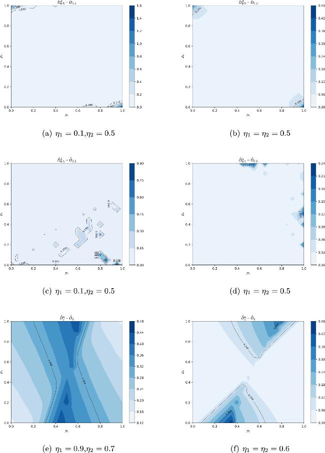
Figure 1. (a) and (b) show the difference between ${{\boldsymbol{D}}}_{\frac{1}{2}}^{{ \mathcal A }}({ \mathcal N }\parallel { \mathcal M })$ and ${{\boldsymbol{D}}}_{\frac{1}{2}}({ \mathcal N }\parallel { \mathcal M })$. (c) and (d) show the difference between ${\tilde{{\boldsymbol{D}}}}_{\frac{1}{2}}^{{ \mathcal A }}({ \mathcal N }\parallel { \mathcal M })$ and ${\tilde{{\boldsymbol{D}}}}_{\frac{1}{2}}({ \mathcal N }\parallel { \mathcal M })$. (e) and (f) show the difference between ${\tilde{{\boldsymbol{D}}}}_{2}^{{ \mathcal A }}({ \mathcal N }\parallel { \mathcal M })$ and ${\tilde{{\boldsymbol{D}}}}_{2}({ \mathcal N }\parallel { \mathcal M })$. We vary the parameters p1 and p2 and fix the parameters η. |
The gap between the amortized channel divergences and the generalized channel divergences displays the advantage of the adaptive strategy over product strategy in determining the sampling complexity for discrimination the generalized amplitude damping channels.
5. Conclusion
This paper is to clarify the problem of the sampling complexity of channel discrimination. That is to say, what is the smallest number of samples needed to ensure that the distinguisher can figure out the unknown channels with a fixed error probability. We have introduced various versions of channel divergences and the definitions of sample complexity of symmetric setting, asymmetric setting, and error exponent setting. As our main results, we have presented the lower and upper bounds of the sampling complexity of channel discrimination. For the product strategy, we have found that these bounds are always characterized in terms of generalized channel divergences. For the adaptive strategy, the bounds are characterized in terms of the amortized channel divergences. Finally, we demonstrate our results by two important classes of channels. On the one hand, for classical-quantum channels, the adaptive strategy can not take advantage over the product strategy in the setting of determining sampling complexity by using of the previous results [16]. On the other hand, for the generalized amplitude damping channels, we conclude that the adaptive strategy does take advantage over the product strategy in the setting of determining the sampling complexity by numerical simulation. We believe that our results confirm the advantage of adaptive strategy and separation from the product strategy for some particular channels.
Appendix A Properties of the channel fidelity
Lemma A.1 Let ${{ \mathcal N }}_{A\to B}$ and ${{ \mathcal M }}_{A\to B}$ be quantum channels. Then we can restrict the infimum to pure states${\varphi }_{RA}\in { \mathcal S }(RA)$ in definition 3, i.e.,
$\begin{eqnarray}\begin{array}{l}{\boldsymbol{F}}({ \mathcal N },{ \mathcal M })\\ \quad =\mathop{\inf }\limits_{{\varphi }_{RA}\in { \mathcal S }(RA)}F({{ \mathcal N }}_{A\to B}({\varphi }_{RA}),{{ \mathcal M }}_{A\to B}({\varphi }_{RA})).\end{array}\end{eqnarray}$
Proof. Suppose that ρRA = ∑ipi∣φi⟩RA⟨φi∣ is an arbitrary ensemble decomposition of mixed state ρRA. We find that
$\begin{eqnarray}\begin{array}{l}F({{ \mathcal N }}_{A\to B}({\rho }_{RA}),{{ \mathcal M }}_{A\to B}({\rho }_{RA}))\\ =\,F({{ \mathcal N }}_{A\to B}(\displaystyle \sum _{i}{p}_{i}| {\varphi }_{i}{\rangle }_{RA}\langle {\varphi }_{i}| ),\\ \quad \,{{ \mathcal M }}_{A\to B}(\displaystyle \sum _{i}{p}_{i}| {\varphi }_{i}{\rangle }_{RA}\langle {\varphi }_{i}| ))\\ =\,F(\displaystyle \sum _{i}{p}_{i}{{ \mathcal N }}_{A\to B}(| {\varphi }_{i}{\rangle }_{RA}\langle {\varphi }_{i}| ),\\ \quad \displaystyle \sum _{i}{p}_{i}{{ \mathcal M }}_{A\to B}(| {\varphi }_{i}{\rangle }_{RA}\langle {\varphi }_{i}| ))\\ \geqslant \displaystyle \sum _{i}{p}_{i}F({{ \mathcal N }}_{A\to B}(| {\varphi }_{i}{\rangle }_{RA}\langle {\varphi }_{i}| ),\\ \quad {{ \mathcal M }}_{A\to B}(| {\varphi }_{i}{\rangle }_{RA}\langle {\varphi }_{i}| ))\\ \geqslant \displaystyle \sum _{i}{p}_{i}\mathop{\min }\limits_{i}F({{ \mathcal N }}_{A\to B}(| {\varphi }_{i}{\rangle }_{RA}\langle {\varphi }_{i}| ),\\ \quad {{ \mathcal M }}_{A\to B}(| {\varphi }_{i}{\rangle }_{RA}\langle {\varphi }_{i}| ))\\ =\,F({{ \mathcal N }}_{A\to B}({\varphi }_{RA}),{{ \mathcal M }}_{A\to B}({\varphi }_{RA})),\end{array}\end{eqnarray}$
where φRA is the optimal pure state in the optimization (A1).The second equality follows from the linear property of quantum channel. The first inequality follows from the joint concavity of fidelity.
Lemma A.2 (Data processing) Let${{ \mathcal N }}_{A\to B}$ and${{ \mathcal M }}_{A\to B}$ be quantum channels. Let Θ be a superchannel as described in (5). Then the following inequality holds
$\begin{eqnarray}{\boldsymbol{F}}({ \mathcal N },{ \mathcal M })\leqslant {\boldsymbol{F}}({\rm{\Theta }}({ \mathcal N }),{\rm{\Theta }}({ \mathcal M })).\end{eqnarray}$
Proof. Let ${{ \mathcal F }}_{C\to D}={\rm{\Theta }}({ \mathcal N })$ and ${{ \mathcal G }}_{C\to D}={\rm{\Theta }}({ \mathcal M })$ be the channels that are output from superchannel Θ. Then we have
$\begin{eqnarray}\begin{array}{l}F({ \mathcal F }({\varphi }_{EC}),{ \mathcal G }({\varphi }_{EC}))\\ =\,F({{ \mathcal V }}_{BR\to D}\circ ({{ \mathcal N }}_{A\to B}\displaystyle \otimes {{ \mathcal I }}_{R})\circ {{ \mathcal U }}_{C\to AR}({\varphi }_{EC}),\\ \quad {{ \mathcal V }}_{BR\to D}\circ ({{ \mathcal M }}_{A\to B}\displaystyle \otimes {{ \mathcal I }}_{R})\circ {{ \mathcal U }}_{C\to AR}({\varphi }_{EC}))\\ =\,F({{ \mathcal V }}_{BR\to D}\circ ({{ \mathcal N }}_{A\to B}\displaystyle \otimes {{ \mathcal I }}_{R})({\eta }_{ARE}),\\ \quad {{ \mathcal V }}_{BR\to D}\circ ({{ \mathcal M }}_{A\to B}\displaystyle \otimes {{ \mathcal I }}_{R})({\eta }_{ARE}))\\ \geqslant F(({{ \mathcal N }}_{A\to B}\displaystyle \otimes {{ \mathcal I }}_{R})({\eta }_{ARE}),({{ \mathcal M }}_{A\to B}\displaystyle \otimes {{ \mathcal I }}_{R})({\eta }_{ARE}))\\ \geqslant {\boldsymbol{F}}({ \mathcal N },{ \mathcal M }),\end{array}\end{eqnarray}$
where ${\eta }_{ARE}={{ \mathcal U }}_{C\to AR}({\varphi }_{EC}))$. The first inequality follows from the data processing property of the state fidelity. The second inequality follows from the fact that ${\eta }_{{ARE}}$ is a particular state, but the fidelity of the channel involves an optimization over all input state.Lemma A.3 (Joint concavity) Let ${{ \mathcal N }}_{A\to B}^{i}$ and ${{ \mathcal M }}_{A\to B}^{i}$ be the quantum channels for all $i\in { \mathcal I }$, and let pi be a probability distribution over the same index set. Then we have
$\begin{eqnarray}{\boldsymbol{F}}(\displaystyle \sum _{i}{p}_{i}{{ \mathcal N }}^{i},\displaystyle \sum _{i}{p}_{i}{{ \mathcal M }}^{i})\geqslant \displaystyle \sum _{i}{p}_{i}{\boldsymbol{F}}({{ \mathcal N }}^{i},{{ \mathcal M }}^{i}).\end{eqnarray}$
Proof. Let $\bar{{ \mathcal N }}={\sum }_{i}{p}_{i}{{ \mathcal N }}^{i}$ and $\bar{{ \mathcal M }}={\sum }_{i}{p}_{i}{{ \mathcal M }}^{i}$. Next, let φ be the optimal state for the definition ${\boldsymbol{F}}(\bar{{ \mathcal N }},\bar{{ \mathcal M }})$, that is ${\boldsymbol{F}}(\bar{{ \mathcal N }},\bar{{ \mathcal M }})=F(\bar{{ \mathcal N }}(\varphi ),\bar{{ \mathcal M }}(\varphi ))$. Then we have
$\begin{eqnarray}\begin{array}{rcl}{\boldsymbol{F}}(\bar{{ \mathcal N }},\bar{{ \mathcal M }}) & = & F(\bar{{ \mathcal N }}(\varphi ),\bar{{ \mathcal M }}(\varphi ))\\ & = & F(\displaystyle \sum _{i}{p}_{i}{{ \mathcal N }}^{i}(\varphi ),\displaystyle \sum _{i}{p}_{i}{{ \mathcal M }}^{i}(\varphi ))\\ & \geqslant & \displaystyle \sum _{i}{p}_{i}F({{ \mathcal N }}^{i}(\varphi ),{{ \mathcal M }}^{i}(\varphi ))\\ & \geqslant & \displaystyle \sum _{i}{p}_{i}{\boldsymbol{F}}({{ \mathcal N }}^{i},{{ \mathcal M }}^{i}).\end{array}\end{eqnarray}$
The first inequality follows from the concavity of state fidelity. The second inequality follows from the definition of the channel fidelity, where we should take infimum over all pure state.Appendix B
Lemma B.2 (Quantum Chernoff bound) For positive semi-definite operator A and B, it holds that [40]
$\begin{eqnarray}\frac{1}{2}[{\rm{Tr}}(A+B)-\parallel A-B{\parallel }_{1}]\leqslant {Q}_{\min }(A\parallel B),\end{eqnarray}$
where ${Q}_{\min }(A\parallel B)=\mathop{\min }\limits_{\alpha \in [0,1]}{\rm{Tr}}[{A}^{\alpha }{B}^{1-\alpha }].$Definition B.3 (Chernoff divergence) For quantum states ρ and σ, the Chernoff divergence is defined as [40]
$\begin{eqnarray}C(\rho \parallel \sigma )=-\mathrm{log}{Q}_{\min }(\rho \parallel \sigma ).\end{eqnarray}$
Lemma B.4 Let ρ and σ be quantum states. Then for α ∈ (1, ∞) and ϵ ∈ (0, 1), it holds that [41]
$\begin{eqnarray}-\mathrm{log}{\beta }_{1}\leqslant {\tilde{D}}_{\alpha }(\rho \parallel \sigma )+\frac{\alpha }{\alpha -1}\mathrm{log}\frac{1}{1-\varepsilon }\end{eqnarray}$
under the constrain α1≤ϵ. Lemma B.5 Let ρ and σ be quantum states. Then for α ∈ (0, 1) and ϵ ∈ (0, 1), it holds that [42]
$\begin{eqnarray}-\mathrm{log}{\beta }_{1}\geqslant {D}_{\alpha }(\rho \parallel \sigma )+\frac{\alpha }{\alpha -1}\mathrm{log}\frac{1}{\varepsilon }\end{eqnarray}$
under the constrain α1≤ϵ. Lemma B.6 [40] Let L and K be positive semi-definite and s ∈ (0, 1). Then,
$\begin{eqnarray}\begin{array}{l}{\rm{Tr}}[{L}^{s}{K}^{1-s}]\geqslant {\rm{Tr}}[K\{L\geqslant K\}]\\ \quad +{\rm{Tr}}[L\{L\lt K\}],\end{array}\end{eqnarray}$
where {L≥K} = I − {L < K} is the projector onto the subspace spanned by eigenvectors corresponding to non-negative eigenvalues of L − K.Appendix C
We define amortized channel divergence as a measure of the distinguishability of two quantum channels, in the sense that, in contrast to the generalized channel divergence defined above, we consider two different states ρRA and ρRA that can be input to the channels ${{ \mathcal N }}_{A\to B}$ and ${{ \mathcal M }}_{A\to B}$, in order to explore the largest distinguishability that can be realized between the channels. However, it is sensible to subtract off the initial distinguishability of the states ρRA and ρRA from the final distinguishability of the channel output states ${{ \mathcal N }}_{A\to B}$ and ${{ \mathcal M }}_{A\to B}$ from a resource-theoretic perspective, since these initial states themselves could have some distinguishability. The amortized channel divergence has many attractive properties [16], such as data-processing inequality, joint convexity, and so on. In particular, the following lemma named as meta-converse, which was initially used to recover particular converse statements for quantum channel discrimination, plays a central role in our proof of the sample complexity with adaptive strategy.
Lemma C.1 (Meta-converse) [16] Let $p={\rm{Tr}}\{{Q}_{n}{\rho }_{n}({S}_{n})\}$ and $q={\rm{Tr}}\{{Q}_{n}{\sigma }_{n}({S}_{n})\}$ be the final decision probabilities corresponding to measurement Qn. Then for adaptive channel discrimination as introduced in section 2.2 , and any faithful general divergence D, we have
$\begin{eqnarray}D(p\parallel q)\leqslant D({\rho }_{n}({S}_{n})\parallel {\sigma }_{n}({S}_{n}))\leqslant n{{\boldsymbol{D}}}^{{ \mathcal A }}({ \mathcal N }\parallel { \mathcal M }).\end{eqnarray}$