


1. Introduction
Quantum optomechanics has been an active field of research for at least the last three decades. It is not coincidental, or a casualty, since there is great interest in obtaining a profound understanding of how systems of different orders of magnitude relate when they are coupled through some designed interaction; leading to use as technological platforms to test quantum effects and measurements in the nanoscale [1]. In the most broad sense, an optomechanical system is composed of a photonic (light) and phononic (matter) subsystems, interacting through a proper degree of freedom. It is of interest when the field, due to radiation pressure exerts a displacement in the boundary of a cavity, amplified and fed back if the boundary can be displaced in some manner, harmonically in most of the cases. Nowadays, there exists a very comprehensive literature on the fundamentals of the optomechanical realm [2–5]. In the traditional approximation, the frequency of the cavity field is modified by the displacement of the mechanical boundary due to this radiation pressure, thus creating a feedback loop between how much the displacement is, and how much conversion between quanta of light and matter takes place due to the dynamical Casimir effect [6–8]. At the heart of this phenomenon, when cavity QED is used to describe it, lays an approximation to the displacement of the boundary. This approximation states that for a resonant cavity of length L, when the instantaneous displacement x is orders of magnitude smaller, we can expand a quotient in a series of contributions, typically keeping to the first order when the number of quanta in the field coupled to the linear displacement of the cavity boundary, leading to a completely integrable system. Due to the expansion of the interaction term, in incremental orders, it naturally motivates asking whether their contributions modify the behavior of the system. Despite the first order of interaction being highly non-linear, it can be linearized using the polaron transformation, a technique not suitable for higher orders due to their disadvantage of disregarding non-vanishing terms, like the quadratic and upper. Archetypical examples of linear and quadratic couplings are the well-known Fabry–Pérot cavity, and the ‘membrane-in-the-middle’cavity [9–11], respectively. Although the linear coupling can be diminished with a well-engineered cavity, the quadratic term is persistent, thus the interest in studying the expansion of the position cavity frequency up-to second order interaction. There exists a plethora of results involving linear and quadratic interaction in optomechanical systems: the so-called optical spring [12], single-photon mechanical control [13], photon blockade in linear and quadratic couplings [14], mechanical cooling [15, 16], implementation of quadratic couplings in circuits [17], preparation of nonclassical states [18], squeezing-enhanced quantum sensing [19], quantum signatures [20], and optomechanically induced transparency [21].
At first, the intention to include the quadratic term responds to the fact that the preservation of harmonic behavior when just linear coupling is considered, has an upper bound; thus, higher regimes preserving the semi-positiveness of the eigenvalues, needs the quadratic and upper orders in the interaction. On the other hand, including dephasing over dissipation is intended to represent, for example, results where gravitational decoherence can be mimicked with pure dephasing optomechanical systems [22–24], this leads to thinking that exploring such optomechanical analogs may shed light on gravitationally induced dephasing dynamics of macroscopic matter-field superposition states, as it was stated in [25]. Moreover, other kinds of related systems, like many-bodies, and quantum dots, may exhibit dephasing [26–28], or in the quantum sensing realm, where testing on the gravity acceleration can be estimated through the phase readout of the field-resonator coupling phase [29]. Thus, capturing information about the dephasing mechanism and its influence on the quantum mechanical systems appears to be natural. Considering the dephasing as the mechanism where energy-preserving damping occurs, it can be thought as a scattering process with interference terms proportional to the number operator of the Hamiltonian, where no energy is lost or gained, just a phase changing in time. This process makes the off-diagonal elements of the density matrix of the system to decay to zero, leading inevitably to a stationary diagonal solution, so no thermalization is taking place, with occupation probabilities preserved and coherence erased. In [30], the phase-damped oscillator to the system exhibits these features, with the specification of using the Lindbladian master equation to describe its characteristics. Here an alternative approach is proposed, which will be equivalent. As dephasing will be relevant, the mechanism devised by Milburn [31], where the assumption that on sufficiently short-time scales the system evolves by a random sequence of unitary phase changes generated by the system’s Hamiltonian, can be thought as a suitable way of dealing with the phase damping. This process, called intrinsic decoherence, has been the subject of numerous studies since its introduction, due to the ability to handle damping in the systems. Despite the former discussion about the background of the proposal [32, 33], and recent inquiries about the suitability of this kind of decoherence as a physical theory [34], we can justify the election as an alternative to modeling a master equation with the Hamiltonian itself as a decaying operator [35]. As a direct antecedent, investigations in a coupled and displaced harmonic oscillator, along a simple moving-mirror system have been done [36–38], but a large corpus of results exists within the literature [39–49]. As a final ingredient in this manuscript, the use of the well-developed non-stationary spectroscopy proposed by Eberly and Wódkiewicz [50] is considered, which has been successfully used for many kinds of system and processes; pure atomic [51–53], atom-field [54, 55], and thermalization process [56, 57]. The advantage of capturing information about the energetic transitions and resonances in the system as a function of time is notable, and whose limit in the long-time is the well-known Wiener–Khinchin power spectrum, it then leads to a natural choice to explore the energetic setting of the system evolution in time. Notably, there have been contributions to resolve the single-photon spectra of the usual optomechanical interaction [58], up to the linear coupling term, resulting in the formation of the well-known sidebands, providing insights on how these features arise. Conjuring the system, the pure dephasing evolution scheme and the spectroscopic visualization process, the proposal of this paper is to ask how the dynamics of an optomechanical system, with linear and quadratic couplings, experiencing a damping due to phase decoherence is presented, and also the spectral response in the evolution of the mechanical system. Particularly, the single-photon influence in the resonator is described, plus a comparison when the cavity field and the resonator are prepared initially in coherent states as well.
The paper is organized as follows: in section 2 we start revisiting the fundamentals of the quantum optomechanical Hamiltonian formulation up to a second order expansion in the interaction, keeping in mind that the treatment is platform-independent as far as we do not specify the interdependency of the coupling strengths. It follows the solution given by diagonalization using unitary transformations. Expectation values measurements are given to discuss the dynamics of the evolution, and how the phase damping induces steady-state in the mechanical resonator. In section 3 we use the non-stationary spectral resolving method of Eberly and Wódkiewicz to determine how the inclusion of the second order interaction modifies the spectral response, and to gain insights into the evolution of energetic transitions when the decoherence ceases the quanta conversion between the cavity field and the mechanical resonator. Finally, a conclusion is given in section 4 to discuss and highlight the findings.
2. Dynamics
The system under study can be thought at first as the quintessential optomechanical cavity, where an electromagnetic field is enclosed by two reflective boundaries, one of them, the mechanical resonator, experiences length displacement L(x) = L − x due to radiation pressure [59, 60], where L is the initial length of the cavity, and x the instantaneous position of the moving boundary, as the scheme depicted in figure 1. In the standard treatment, this length determines the optical frequencies ω(x) = 2πc/L(x) coupled to the cavity field $\hat{n}$. Suppose the mechanical resonator has a natural frequency ωm, the interacting system at large is given by $\omega (\hat{x})\hat{n}+{\omega }_{m}\hat{N}$. The quantization of $\omega (\hat{x})$, with $\hat{x}\propto {\hat{b}}^{\dagger }+\hat{b}$ is very subtle, with two approaches emerging: (1) the phenomenological considering just the moving mirror movement, leading to the well-known linear and quadratic interaction, and (2) the Hamiltonian approach [10], which can be considered the real form, since it deals with the precise boundary conditions of the problem. Here we will follow the usual phenomenological approach, where the quantization of the mirror movement is done under the assumption of small perturbations on the mechanical motion, are shorter than the optical wavelength inside the cavity. In this setting, the intracavity can adiabatically follow the mirror movements because it can learn the states of the interaction in times shorter than 1/ωm.
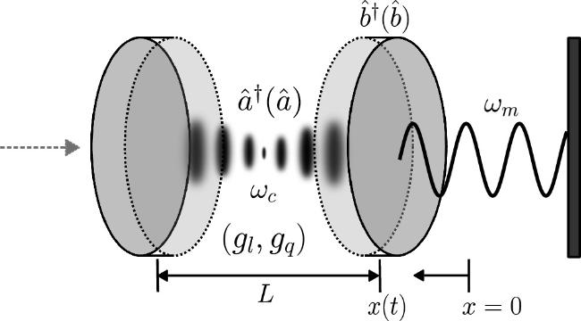
Figure 1. Schematic representation of an optomechanical cavity sustaining an electromagnetic field ${\hat{a}}^{\dagger }(\hat{a})$ with frequency ωc, which is coupled to a mechanical resonator (reflecting moving mirror) ${\hat{b}}^{\dagger }(\hat{b})$ with frequency ωm. The coupling is denoted as a function of the linear and quadratic contributions gl and gq. |
Here, the usual commutation relations from bosonic algebra for the field and the mirror take place, $[\hat{a},{\hat{a}}^{\dagger }]\,=[\hat{b},{\hat{b}}^{\dagger }]=1$. Based on the arguments above, and assuming the timescale in favor of the field, we expand the denominator of the optical frequency in terms of $\hat{x}\ll L$, where $\hat{x}$ represents the quantized version of the mirror position, then we arrive at a series of contributions
$\begin{eqnarray}\omega (\hat{x})={\omega }_{c}\displaystyle \sum _{k=0}^{\infty }{\left(\frac{L}{\hat{x}}\right)}^{k},\end{eqnarray}$
where ωc is the proper frequency of the cavity field. This leads us to consider, along the fundamental term, the two-relevant k = 1 and 2, representing linear and quadratic contributions to the optical frequency modification due to radiation feedback on-and-from the mechanical resonator. The kind of perturbations the mirror can experience to sustain the photon-phonon conversion, is bounded to those behaving harmonically at first, since it can be shown that non-harmonically motion, like linear uniform movement [8, 61–63], does not lead to dynamical Casimir effect, thus the conversion between photons and phonons due radiation pressure will be negligible.Finally, let us define the Hamiltonian of the system under these considerations as free and int , the free and linear-quadratic interaction Hamiltonians are explicitly given by
$\begin{eqnarray}\hat{H}={\hat{H}}_{{\mathtt{free}}}+{\hat{H}}_{{\mathtt{int}}}^{(l)}+{\hat{H}}_{{\mathtt{int}}}^{(q)},\end{eqnarray}$
with $\begin{eqnarray}\begin{array}{rcl}{\hat{H}}_{{\mathtt{free}}} & = & {\omega }_{c}\hat{n}+{\omega }_{m}\hat{N},\\ {\hat{H}}_{{\mathtt{int}}}^{(l)} & = & -{g}_{l}\hat{n}\left({\hat{b}}^{\dagger }+\hat{b}\right),\\ {\hat{H}}_{{\mathtt{int}}}^{(q)} & = & {g}_{q}\hat{n}{\left({\hat{b}}^{\dagger }+\hat{b}\right)}^{2},\end{array}\end{eqnarray}$
in which the interaction strength gl and gq will be platform-independent, allowing different realizations of the Hamiltonian, like optomechanical cavities or superconducting circuits [17, 59]. In [64], it is shown how the standard and non-standard quadratic terms arise in consideration under regimes of strong coupling (ωm/ωc) > 1, and even in weak coupling ωm ≪ ωc when non-standard quadratic term is present. Since non-standard and standard quadratic terms take care of the momentum exchange and conservation, its analysis is of importance. Moreover, the spectral response, will show signatures of the presence of these highly non-linear terms, beyond the usual perturbative method of linearization. In [65], it is shown how the linear optomechanical Hamiltonian is not bounded from below for sufficient large number of photons, violating the requirement $\langle \omega (\hat{x})\hat{n}\rangle \geqslant 0$, which implies that higher orders of interaction must be needed. [66] shows this from the point of view of out-of-equilibrium thermodynamics of the optomechanical system.Diagonalization
When a standard linear coupling optomechanical system is considered, the most suitable weak-coupling methods is of linearization (small classical perturbations to the quantum mechanical quantities), but as it was shown in some works [67], this procedure cannot catch the non-linear behavior of strong-coupling between light and matter, furthermore, it can lead to non-physical scenarios. This system, with linear and quadratic coupling has been addressed previously, using Lie algebraic methods to determine its temporal evolution when linear strong coupling is considered [68], also the temporal evolution of the linear-quadratic coupling when a forcing term in the cavity field is introduced [69]. In this work, the diagonalization of equations (2 )–(3 ) is done using unitary transformations, a one-mode squeezing and a one-mode displacement, in the mechanical resonator basis $\{\hat{b},{\hat{b}}^{\dagger }\}$. Thus, applying the following operators diag ) Hamiltonian,
$\begin{eqnarray}\begin{array}{rcl}\hat{S}(r(\hat{n})) & = & \exp \left[\frac{1}{2}r(\hat{n})\left({\hat{b}{}^{\dagger }}^{2}-{\hat{b}}^{2}\right)\right],\\ \quad \hat{D}(\alpha (\hat{n})) & = & \exp \left[\alpha (\hat{n})\left({\hat{b}}^{\dagger }-\hat{b}\right)\right],\end{array}\end{eqnarray}$
we arrive at the diagonalized ( $\begin{eqnarray}\begin{array}{rcl}{\hat{H}}_{{\mathtt{diag}}} & = & {\omega }_{c}\hat{n}+{\bar{\omega }}_{m}(\hat{n})\hat{N}-{\bar{\omega }}_{m}(\hat{n})| \alpha (\hat{n}){| }^{2}\\ & = & {\omega }_{c}\hat{n}+{\bar{\omega }}_{m}(\hat{n})\hat{N}-\frac{{g}_{l}^{2}{\hat{n}}^{2}{{\rm{e}}}^{-2r(\hat{n})}}{{\bar{\omega }}_{m}(\hat{n})},\end{array}\end{eqnarray}$
where quantities emerge proportionally to the number of photons $\hat{n}$, carrying the information about the field inside the cavity, these are $\begin{eqnarray}\begin{array}{rcl}r(\hat{n}) & = & \frac{1}{4}\mathrm{ln}\left|1+\frac{4{g}_{q}\hat{n}}{{\omega }_{m}}\right|,\\ {\bar{\omega }}_{m}(\hat{n}) & = & \sqrt{{\omega }_{m}\left({\omega }_{m}+4{g}_{q}\hat{n}\right)},\\ \quad \alpha (\hat{n}) & = & -\frac{{g}_{l}\hat{n}{{\rm{e}}}^{-r}}{{\bar{\omega }}_{m}(\hat{n})}.\end{array}\end{eqnarray}$
Note as well the appearance of a quadratic number of photons operator ${\hat{n}}^{2}$, this can be interpreted as a Kerr-like medium inside the cavity, which is responsible for non-linear effects.Having the diagonalized expression (5 ), we can return to the original reference frame using the inverse transformations,
$\begin{eqnarray}\begin{array}{rcl}{\hat{H}}_{{\mathtt{diag}}} & \equiv & \hat{D}(\alpha (\hat{n}))\hat{D}(r(\hat{n}))\,\hat{H}\,{\hat{S}}^{\dagger }(r(\hat{n})){\hat{D}}^{\dagger }(\alpha (\hat{n}))\\ & \Rightarrow & \hat{H}={\hat{S}}^{\dagger }(r(\hat{n})){\hat{D}}^{\dagger }(\alpha (\hat{n}))\,{\hat{H}}_{{\mathtt{diag}}}\,\hat{D}(\alpha (\hat{n}))\hat{S}(r(\hat{n})).\end{array}\end{eqnarray}$
A complete survey on the diagonalization procedure can be found in the appendix . The form in equation (7 ) arises naturally from the diagonalization procedure, its action $\hat{H}| \psi \rangle $ will lead to the application of displaced squeezed states, which are different from the squeezed coherent states, since $\hat{D}(\alpha (\hat{n}))\hat{S}(r(\hat{n}))\ne \hat{S}(r(\hat{n}))\hat{D}(\alpha (\hat{n}))$. Choose, for example ∣ψ⟩ = ∣n, 0⟩, this is a Fock number state in the cavity field, and zero mechanical excitations, we obtain 5 ), defined as ${{ \mathcal E }}_{n,N}={\omega }_{c}n+{\bar{\omega }}_{m}(n)N-{\bar{\omega }}_{m}(n)| \alpha (n){| }^{2}$, for $n,N\in {\mathbb{N}}$. Panels A and B show the energy levels when ωc = ωm, fixing gq and variating gl and vice versa, respectively. We can see that the only uncoupled non-degenerate level is ${{ \mathcal E }}_{0,0}$; this degeneracy of levels is broken as gl grows in panel A, but it is broken as soon as gq ≠ 0 in panel B. On the other hand, panels C and D show the energy levels when ωm ≪ ωc, fixing one of the couplings and variating the other. Here the degeneracy of levels is totally broken from the start, showing crossings at some specific values of gl and gq. Note that fixing gq and variating gl in panel C can lead to a triple level crossing.
$\begin{eqnarray*}\langle n,0| \hat{H}| n,0\rangle ={\omega }_{c}n+{\omega }_{m}{ \mathcal G }(r(n),\alpha (n))-{\bar{\omega }}_{m}(n)| \alpha (n){| }^{2},\end{eqnarray*}$
where function ${ \mathcal G }$ emerges as the expectation value $\begin{eqnarray*}\langle r(n),\alpha (n)| \hat{N}| r(n),\alpha (n)\rangle =| \alpha (n){| }^{2}+{\sinh }^{2}r(n),\end{eqnarray*}$
where ∣r(n), α(n)⟩ are displaced squeezed states, denoting clearly the processes of displacement and squeezing taking place in the Hamiltonian. In figure 2, the eigenvalues of (Dissipation and dephasing in optomechanical systems
Dissipation refers to the energy lost in a system, whereas dephasing is a mechanism that preserves the population, and thus no net energy loss is observed. In both mechanism, decoherence is observed. In optomechanical systems, dissipation affects the mechanical and optical susceptibility due to the interaction between the cavity field and mechanical modes, in this sense, photonic dissipation usually dominates; however, if mechanical dissipation is higher, it can lead to a feedback force on the electromagnetic mode, causing amplification or damping [70]. It is a well-known fact that dissipation has a more detrimental effect on quantum systems compared to dephasing, as it involves energy loss and can significantly disrupt quantum coherence. Dephasing, while still disruptive, primarily affects the relative phases and can be less damaging. To favor dephasing over dissipation, one could focus on minimizing energy exchanges with the environment. This can be achieved by controlling the interaction parameters and environmental coupling. Moreover, understanding the time scales is crucial, as dissipation typically occurs over a longer timescale compared to dephasing, suggesting that short-time interactions might help in reducing dissipation effects [71]. The dissipation processes affecting an optomechanical system include photon leakage through mirrors and spin ensemble dissipation. Dephasing can negatively impact phenomena such as photon blockade and photon antibunching. Pure dephasing has been observed and analyzed in mechanical quantum resonators, highlighting its significance in the study of optomechanical systems [72]. Observing the conditions needed for dissipation to be diminished in favor of dephasing, we can proceed to propose how to model this mechanism of decoherence. While dissipation is a primary mechanism of decoherence, it may be overlooked in certain scenarios involving short-time evolution. In these situations, dephasing becomes a valuable resource for utilizing new quantum features. In this sense, we can mention how dephasing can enable fast charging of quantum batteries [73], the effects of dephasing in quantum conductors [74], investigations on how dephasing can be distinguished in quantum and classical Markovian approaches [75], the decoherence in squeezed mechanical oscillators [76], the synthesis of mechanical NOON states in ultrastrong optomechanics [77], or the classical and quantum coherence in microresonators under ultrastrong coupling [78, 79].
What dephasing models do we have?
The decoherence of the system is usually described by master equations, which are derived using reasonable statistical assumptions and specific but arbitrary models to simulate the environment and its interaction with the system [80]. Conceptually, it is debatable why one has to invoke the environment, dissipation, or the measuring apparatus to conclude that coherent states lead to statistical mixtures under bath interactions. Efforts in other kinds of model, while not as successful as the master equations, have the modification of standard quantum mechanics as a goal so that decoherence becomes intrinsic, i.e., not related to any specific model of interaction or entanglement with the Universe. For example, in [81] the Schrödinger equation is modified phenomenologically by adding non-linear terms to the Hamiltonian so that the system, at Poisson distributed times, undergoes a sudden localization, where the model contains two unspecified parameters: the frequency and the spatial extent of localization. However, it has the feature that the energy of the system is not preserved. A scheme for decoherence has been proposed [82], assuming a finite difference Liouville equation with time step, τ, which has been connected to the time energy uncertainty relation. It has been shown that this finite difference equation is equivalent to a semigroup master equation of the Lindblad form. Finally, in Milburn's proposal, previously related to [31], time is a parameter, as in standard quantum mechanics, along with the Poisson distribution which is assumed. This parametric dependence in Milburn’s proposal is one of the strongest features of this decoherence mechanism, in addition, it has been shown that it is equivalent to a Lindbladian master equation up to second order. As a conclusion in this regard, recently a debate whether intrinsic decoherence models are physically viable has been raised in [34], using arguments from the quantum parameter estimation theory. The conclusion reveals that in some manner, these kind of models can be falsifiable when they are implemented indiscriminately to represent decoherence without a careful bounding in the parameters of the evolution and dephasing rate. Later in the paper, a comparison between the evolution given by the intrinsic decoherence model, and the master equation with decaying operator proportional to the Hamiltonian [83], will serve as a point of comparison between both approaches.
Intrinsic decoherence
Now, according to Milburn [31], we can define the evolution of a wavefunction in the intrinsic decoherence framework by
$\begin{eqnarray}{\hat{\rho }}_{\gamma }(t)={{\rm{e}}}^{-\gamma t}\displaystyle \sum _{k=0}^{\infty }\frac{{\left(\gamma t\right)}^{k}}{k!}{\left(| {\psi }_{k}\rangle \langle {\psi }_{k}| \right)}_{\gamma },\end{eqnarray}$
where the k-th ket is given by $\begin{eqnarray}{| {\psi }_{k}\rangle }_{\gamma }={{\rm{e}}}^{-\frac{{\rm{i}}k}{\gamma }\hat{H}}| \psi (0)\rangle ,\end{eqnarray}$
in which the quantity γ represents the rate of decoherence, determining the slope of the damping in the excitation-conserving evolution of the systems’phase. We can also write down the evolution operator of the decoherence as $\begin{eqnarray}{\hat{{ \mathcal U }}}_{\gamma }(t)={{\rm{e}}}^{-\gamma t}\displaystyle \sum _{k=0}^{\infty }\frac{{(\gamma t)}^{k}}{k!}\hat{{ \mathcal V }}\left(\frac{k}{\gamma }\right),\end{eqnarray}$
where $\hat{{ \mathcal V }}(k/\gamma )$ is the k-th component of the evolution operator, given by $\begin{eqnarray}\hat{{ \mathcal V }}\left(\frac{k}{\gamma }\right)={\hat{S}}^{\dagger }(r(\hat{n})){\hat{D}}^{\dagger }(\alpha (\hat{n}))\,{{\rm{e}}}^{-\frac{{\rm{i}}k}{\gamma }{\hat{H}}_{{\mathtt{diag}}}}\hat{S}(r(\hat{n}))\hat{D}(\alpha (\hat{n})).\end{eqnarray}$
A rise of warning must be placed here. Since an infinite sum must be done to obtain the final expression in time, we need to first perform the respective action on the intended operator, and then the sum. Previously, an attempt to describe the evolution of the linear coupling optomechanical interaction [38] settles a precedent on what we can expect, at least looking at the mirror’s response to the phase damping.Since the Hamiltonian (3 ) determines the energetic disposition of the system, the first interest is to determine the time evolution of the dynamical quantities, like the number of phonons and position quadrature of the mirror, parametrically dependent on the decoherence rate γ. This election is justified by the fact that the evolution operator of the decoherence (10 ) via the ${\hat{H}}_{{\mathtt{diag}}}$, commutes with the number of photons operator $\hat{n}$, so looking at the response of the mirror to the cavity field, seems appropriate. Let us start calculating the mechanical bosonic operators in the (k/γ)-representation given by the application of (11 ). To this aim, we need to determine the representation of the bilateral action, 10 ), and the limit γ → ∞ is taken, the expressions reduce to those obtained under the usual Heisenberg evolution. Compare it with those in the appendix (A14 ). Having these expressions, we can compute the time-evolved operator for the number of phonons,
$\begin{eqnarray}\hat{{ \mathcal O }}\left(\frac{k}{\gamma }\right)={\hat{{ \mathcal V }}}^{\dagger }\left(\frac{k}{\gamma }\right)\,\hat{{ \mathcal O }}\,\hat{{ \mathcal V }}\left(\frac{k}{\gamma }\right).\end{eqnarray}$
The calculation involves five steps where we reverse the representation to the original frame of reference. Acting over $\{{\hat{b}}^{\dagger },\hat{b}\}$, we obtain $\begin{eqnarray}\begin{array}{rcl}{\hat{b}}^{\dagger }\left(\frac{k}{\gamma }\right) & = & {\hat{b}}^{\dagger }\,{\chi }_{1}^{(n)}\left(\frac{k}{\gamma }\right)+\hat{b}\,{\chi }_{2}^{(n)}\left(\frac{k}{\gamma }\right)+{\chi }_{3}^{(n)}\left(\frac{k}{\gamma }\right),\\ \hat{b}\left(\frac{k}{\gamma }\right) & = & \hat{b}\,{\chi }_{1}^{(n)}{\left(\frac{k}{\gamma }\right)}^{* }+{\hat{b}}^{\dagger }\,{\chi }_{2}^{(n)}{\left(\frac{k}{\gamma }\right)}^{* }+{\chi }_{3}^{(n)}{\left(\frac{k}{\gamma }\right)}^{* },\end{array}\end{eqnarray}$
where the companion coefficients are $\begin{eqnarray}\begin{array}{rcl}{\chi }_{1}^{(n)}\left(\frac{k}{\gamma }\right) & = & {\cosh }^{2}r(\hat{n})\,{{\rm{e}}}^{\frac{{\rm{i}}k{\bar{\omega }}_{m}(\hat{n})}{\gamma }}\\ & & -\,{\sinh }^{2}r(\hat{n})\,{{\rm{e}}}^{-\frac{{\rm{i}}k{\bar{\omega }}_{m}(\hat{n})}{\gamma }},\\ {\chi }_{2}^{(n)}\left(\frac{k}{\gamma }\right) & = & \frac{1}{2}\left({{\rm{e}}}^{\frac{{\rm{i}}k{\bar{\omega }}_{m}(\hat{n})}{\gamma }}-{{\rm{e}}}^{-\frac{{\rm{i}}k{\bar{\omega }}_{m}(\hat{n})}{\gamma }}\right)\sinh \,2r(\hat{n}),\\ {\chi }_{3}^{(n)}\left(\frac{k}{\gamma }\right) & = & \alpha (\hat{n})\left(\cosh \,r(\hat{n})\,{{\rm{e}}}^{\frac{{\rm{i}}k{\bar{\omega }}_{m}(\hat{n})}{\gamma }}\right.\\ & & \left.-\,\sinh \,r(\hat{n})\,{{\rm{e}}}^{\frac{-{\rm{i}}k{\bar{\omega }}_{m}(\hat{n})}{\gamma }}-{{\rm{e}}}^{-r(\hat{n})}\right).\end{array}\end{eqnarray}$
When each of these coefficients are summed up according to ( $\begin{eqnarray}\begin{array}{rcl}{\hat{N}}_{\gamma }(t) & = & \hat{N}\left({\zeta }_{1}^{(n)}(t)+{\zeta }_{2}^{(n)}(t)\right)+{\hat{b}{}^{\dagger }}^{2}\,{\zeta }_{12}^{(n)}(t)+{\hat{b}}^{2}\,{\zeta }_{12}^{(n)}{(t)}^{* }\\ & & +{\hat{b}}^{\dagger }\left({\zeta }_{13}^{(n)}(t)+{\zeta }_{23}^{(n)}{(t)}^{* }\right)+\hat{b}\left({\zeta }_{23}^{(n)}(t)+{\zeta }_{13}^{(n)}(t)\right)\\ & & +{\zeta }_{2}^{(n)}(t)+{\zeta }_{3}^{(n)}(t),\end{array}\end{eqnarray}$
where the companion terms are given by $\begin{eqnarray}\begin{array}{rcl}{\zeta }_{l}^{(n)}(t) & = & {{\rm{e}}}^{-\gamma t}\displaystyle \sum _{k=0}^{\infty }\frac{{(\gamma t)}^{k}}{k!}\,\left|\right.{\chi }_{l}^{(n)}\left(\frac{k}{\gamma }\right){\left|\right.}^{2},\\ {\zeta }_{lm}^{(n)}(t) & = & {{\rm{e}}}^{-\gamma t}\displaystyle \sum _{k=0}^{\infty }\frac{{(\gamma t)}^{k}}{k!}\,{\chi }_{l}^{(n)}\left(\frac{k}{\gamma }\right){\chi }_{m}^{(n)}{\left(\frac{k}{\gamma }\right)}^{* }.\end{array}\end{eqnarray}$
And the position quadrature $\begin{eqnarray}\begin{array}{rcl}{\hat{X}}_{\gamma }(t) & = & {\hat{b}}^{\dagger }\left({\nu }_{1}^{(n)}(t)+{\nu }_{2}^{(n)}{(t)}^{* }\right)+\hat{b}\left({\nu }_{1}^{(n)}{(t)}^{* }\right.\\ & & \left.+{\nu }_{2}^{(n)}(t)\right)+2{\rm{Re}}\left\{{\nu }_{3}^{(n)}(t)\right\},\end{array}\end{eqnarray}$
where the companion terms are given by $\begin{eqnarray}{\nu }_{l}^{(n)}(t)={{\rm{e}}}^{-\gamma t}\displaystyle \sum _{k=0}^{\infty }\frac{{(\gamma t)}^{k}}{k!}\,{\chi }_{l}^{(n)}\left(\frac{k}{\gamma }\right).\end{eqnarray}$
In the previous set of equations, the superscript (n) denotes a direct play of the number of photons in the cavity field, modifying each term where it appears. Moreover, the frequency of the field is not explicitly apparent in any of the dynamical expressions for the mechanical resonator. Now, it is just a matter of selecting a suitable initial condition. For this, we can start looking at the behavior of a single excitation in the cavity field [13, 15], searching for insights about the transfer of radiation pressure to the mirror in the presence of linear, quadratic and linear-quadratic coupling, parametrically dependent on the decoherence rate γ. Setting number states in the field and the mirror, ∣n, m⟩, with just a single photon $\bar{n}=1$ and no phonons $\bar{N}=0$, this is ∣ψ(0)⟩num = ∣1⟩c ⨂ ∣0⟩m. In figure 3, we see how the system evolves under different circumstances: A. 1 and A. 2 is a linear only coupling, gq = 0, where the number of phonons and the position quadrature are the same, thus the one photon radiation pressure is back and forth between the mirror and the cavity. Turning on the decoherence rate, induces monotonically decreasing of the amplitude, leading to a mean phonon number and quadrature position of $\bar{N}=2$ and $\bar{X}=2$, respectively. B. 1 and B. 2 is a quadratic only coupling, gl = 0, here the number of phonons behaves in almost the same way as the linear coupling, but accelerating the decreasing of amplitude converging to a mean value of $\bar{N}=0.4$, on the other hand, the position quadrature is always null, $\bar{X}(t)=0\ \forall t$, meaning that the mirror is not experiencing back and forth due to radiation pressure, the initial photon is elastically bouncing to a fixed boundary. This behavior is a consequence of the quadratic coupling, which modifies the potential term of the mechanical resonator, breaking its symmetry when the linear term is not included, meaning that the highly non-linear effect of squeezing and two-mode photon-phonon conversion dominates the evolution [84]. Finally, C. 1 and C. 2 accounts for the presence of both the linear and quadratic couplings simultaneously, where we see the presence of double modulation in the number of phonons, indicating squeezing of states. On the other hand, the position quadrature behaves very clean, modulating a decreasing amplitude converging to a mean value. To end this section, we also look at the evolution considering coherent states, in the cavity field and the mirror. For this, we can set the initial condition using the coherent representation of states in the mirror, and the photon distribution in the field, ${| \alpha ,\beta \rangle }_{{\rm{coh}}}={{\rm{e}}}^{-{\alpha }^{2}}{\sum }_{k=0}^{\infty }({\alpha }^{2k}/k!)\,| n,\beta \rangle $. Taking this, and using (15 ) and (17 ), we can obtain the respective behavior, which is shown in figure 4, observing the same label system. Here, a well-known feature of the presence of a quadratic coupling is the revival-like of mean quantities, shown by the optical spring of Rai and Agarwal [12]. We see that the decoherence has an effect of cooling the mirror, thus leading to a mean phonon value $\bar{N}$, without the chance of more revival-like cycles. We can see that the dephasing process leads to the steady-state of the mechanical resonator, when a sufficiently large observation time takes place, it will evolve to some mean phonon value ${\bar{N}}_{\gamma }$ and position quadrature ${\bar{X}}_{\gamma }$. Halting the movement of the resonator, it is equivalent to preventing the dynamical Casimir effect, so features like anti-damping and self-sustained oscillations are not expected within this mechanism, as it is the case in Lindbladian treatment of adiabatic elimination [85].
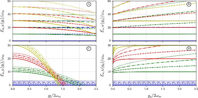
Figure 2. Eigenvalues ${{ \mathcal E }}_{n,N}({g}_{l},{g}_{q})$ of the Hamiltonian ( |

Figure 3. ${\hat{N}}_{\gamma }(t)$ and ${\hat{X}}_{\gamma }(t)$. {A, B, C}. {1, 2} are evolutions with linear, quadratic and linear-quadratic couplings, respectively. Setting ωc = ωm = 1.0, gl = gq = 1.0 and ∣ψ(0)⟩num = ∣1, 0⟩. We see how the decoherence rate γ influences in the diminishing of the amplitude in the three regimes. |

Figure 4. ${\hat{N}}_{\gamma }(t)$ and ${\hat{X}}_{\gamma }(t)$. {A, B, C}. {1, 2} are evolutions with linear, quadratic and linear-quadratic couplings, respectively. Setting ωc = ωm = 1.0, gl = gq = 1.0 and ∣ψ(0)⟩coh = ∣2, 2⟩. We see how the decoherence rate γ influences in the diminishing of the amplitude in the three regimes. |
Dephasing in master equation
As was shown in [35], and more recently in [34] and references therein, the intrinsic decoherence mechanism is equivalent, up to a second order expansion, to a master equation evolving under its Hamiltonian. Take the Poisson model, $\dot{\hat{\rho }}(t)=\gamma \left({{\rm{e}}}^{-{\rm{i}}\hat{H}/\gamma }\hat{\rho }{{\rm{e}}}^{{\rm{i}}\hat{H}/\gamma }-\hat{\rho }\right)$ of the intrinsic decoherence mechanism and expand it in terms of the dephasing rate γ−1, it is such that
$\begin{eqnarray*}\gamma \left({{\rm{e}}}^{-{\rm{i}}\hat{H}/\gamma }\hat{\rho }{{\rm{e}}}^{{\rm{i}}\hat{H}/\gamma }-\hat{\rho }\right)\displaystyle {\overset{{ \mathcal O }{({\gamma }^{-1})}^{2}}{\to }}-{\rm{i}}\left[\hat{H},\hat{\rho }\right]-\frac{1}{2}{\gamma }^{-1}\left[\hat{H},\left[\hat{H},\hat{\rho }\right]\right]\end{eqnarray*}$
which is equivalent to a master equation with jump operators $\hat{J}=\sqrt{\eta }\hat{H}$, with η the strength of the collapse, whose role it is to make phase changes in the time evolution of the observables, conserving the initial population $\langle \hat{\rho }(0)\rangle $, creating a dephasing mechanism. In this case, the relation between η and γ is proportional to η ∝ 1/γ. Here we have to agree with the claims in [34], to be cautious in demands that the intrinsic decoherence model for dephasing is absolutely valid, instead, we align with the argument that for some parameters it will lead to sufficiently good insights about the mechanism of dephasing in dissipationless systems.Spectral characteristics
A direct antecedent of spectral response in and the optomechanical system is the work by Mirza and van Enk [58], where they look at the time-dependent spectrum formation of the single-photon regime in the linear coupling. Their goal was to show how the red and blue sidebands form in time, revealing the energetic mechanism responsible for this response. Heinisch et al [86] use this technique to show the quality of his model for the generation of high-quality single photons using optical resonant cavities. Barbhuiya obtains the spectral response of the vibrational polaritonic modes in optomechanical cavities [87], as a way to determine how anharmonicities to the optical cavity establishes a modified splitting dynamic in the absorption spectrum. We can count other examples, like in the optomechanical mass spectroscopy [88] and bulk crystalline optomechanics [89], where spectral formation plays a prominent role in unraveling the energetic characteristics of the system in consideration. With these antecedents, we can think about the information that the time-dependent spectrum can give us when the dephasing is occurring. Since this decoherence mechanism is time-dependent, it appears that using this spectroscopical technique is natural. Moreover, as we just saw, dephasing leads the system to its steady-state for a sufficiently long-running time. For this case, we may ask about the resolved spectrum what we can obtain in the long-time limit of the analytical expressions. Our next task is, then, to obtain the spectral response of the mechanical resonator, as a way to understand how it deals with the loss of coherence due dephasing.
3. Spectral response
Obtaining the time-dependent spectrum of the mechanical resonator is straight-forward, since the two-time correlation enables us to use the coefficients given by the terms ${\nu }_{l}^{(n)}(t)$ in equation (18 ), which are self-dependent, meaning that $({\chi }_{l}^{(n)}(k/\gamma ))* \to ({\nu }_{l}^{(n)}(t))* $. The time-dependent spectrum is defined by [50],
$\begin{eqnarray}{{ \mathcal S }}_{\gamma }({\rm{\Gamma }},\omega ;t)=2{\rm{\Gamma }}{{\rm{e}}}^{-2{\rm{\Gamma }}t}{\int }_{0}^{t}{\rm{d}}{t}_{1}\,{{\rm{e}}}^{({\rm{\Gamma }}-{\rm{i}}\omega ){t}_{1}}{\int }_{0}^{t}{\rm{d}}{t}_{2}{{\rm{e}}}^{({\rm{\Gamma }}+{\rm{i}}\omega ){t}_{2}}\langle {\hat{b}}_{\gamma }^{\dagger }({t}_{1}){\hat{b}}_{\gamma }({t}_{2})\rangle ,\end{eqnarray}$
where the correlation function for an arbitrary initial condition ∣ψ(0)⟩ is $\begin{eqnarray}\begin{array}{rcl}\langle {\hat{b}}_{\gamma }^{\dagger }({t}_{1}){\hat{b}}_{\gamma }({t}_{2})\rangle & = & \langle \psi (0)| \left[\hat{N}\left[{\nu }_{1}^{(n)}({t}_{1}){\nu }_{1}^{(n)}{({t}_{2})}^{* }\right.\right.\\ & & \left.+\,{\nu }_{2}^{(n)}({t}_{1}){\nu }_{2}^{(n)}{({t}_{2})}^{* }\right]\\ & & +\,{\hat{b}{}^{\dagger }}^{2}\,{\nu }_{2}^{(n)}({t}_{1}){\nu }_{1}^{(n)}{({t}_{2})}^{* }\\ & & +\,{\hat{b}}^{2}\,{\nu }_{1}^{(n)}({t}_{1}){\nu }_{1}^{(n)}{({t}_{2})}^{* }\\ & & +\,{\hat{b}}^{\dagger }\left[{\nu }_{1}^{(n)}({t}_{1}){\nu }_{3}^{(n)}{({t}_{2})}^{* }+{\nu }_{3}^{(n)}({t}_{1}){\nu }_{2}^{(n)}{({t}_{2})}^{* }\right]\\ & & +\,\hat{b}\left[{\nu }_{2}^{(n)}({t}_{1}){\nu }_{3}^{(n)}{({t}_{2})}^{* }+{\nu }_{3}^{(n)}({t}_{1}){\nu }_{1}^{(n)}{({t}_{2})}^{* }\right]\\ & & \left.+\,{\nu }_{2}^{(n)}({t}_{1}){\nu }_{2}^{(n)}{({t}_{2})}^{* }+{\nu }_{3}^{(n)}({t}_{1}){\nu }_{3}^{(n)}{({t}_{2})}^{* }\right]| \psi (0)\rangle .\end{array}\end{eqnarray}$
Looking at the structure of the products of ${\nu }_{l}^{(n)}({t}_{m})$, we can assert that the fundamental need is to calculate the integrals
$\begin{eqnarray}{\int }_{0}^{t}{\rm{d}}{t}_{1}{{\rm{e}}}^{({\rm{\Gamma }}-{\rm{i}}\omega ){t}_{1}}{\int }_{0}^{t}{\rm{d}}{t}_{2}\,{{\rm{e}}}^{({\rm{\Gamma }}+{\rm{i}}\omega ){t}_{2}}{\nu }_{j}^{(n)}({t}_{1}){\nu }_{k}^{(n)}({t}_{2}),\,j,k\in \{1,2,3\}.\end{eqnarray}$
But, if we look at the index condition $j=k\in \left\{1,2,3\right\}\equiv l$, the relation is reduced to $\begin{eqnarray}{\left|{\int }_{0}^{t}\,{\rm{d}}\tau \,{{\rm{e}}}^{({\rm{\Gamma }}-{\rm{i}}\omega )\tau }{\nu }_{l}^{(n)}(\tau )\right|}^{2},\end{eqnarray}$
denoting that in the final instance, the evaluation of the three integrals is all that we need at this point, explicitly given as an operator functional of $\hat{n}$ by $\begin{eqnarray}\begin{array}{rcl} & & {\displaystyle \int }_{0}^{t}\,{\rm{d}}\tau \,{{\rm{e}}}^{({\rm{\Gamma }}-{\rm{i}}\omega )\tau }\,{\nu }_{1}^{(\hat{n})}(\tau )\\ & & \quad =\frac{{{\rm{e}}}^{t\left(\gamma {E}_{\gamma }(\hat{n})+({\rm{\Gamma }}-{\rm{i}}\omega )\right)}-1}{\gamma {E}_{\gamma }(\hat{n})+({\rm{\Gamma }}-{\rm{i}}\omega )}{\cosh }^{2}r(\hat{n})\\ & & \quad -\frac{{{\rm{e}}}^{t\left(\gamma {E}_{\gamma }{(\hat{n})}^{* }+({\rm{\Gamma }}-{\rm{i}}\omega )\right)}-1}{\gamma {E}_{\gamma }{(\hat{n})}^{* }+({\rm{\Gamma }}-{\rm{i}}\omega )}{\sinh }^{2}r(\hat{n})\equiv {{ \mathcal L }}_{1}^{(\hat{n})}(t),\\ & & {\displaystyle \int }_{0}^{t}\,{\rm{d}}\tau \,{{\rm{e}}}^{({\rm{\Gamma }}-{\rm{i}}\omega )\tau }\,{\nu }_{2}^{(\hat{n})}(\tau )=\frac{1}{2}\left[\frac{{{\rm{e}}}^{t\left(\gamma {E}_{\gamma }(\hat{n})+({\rm{\Gamma }}-{\rm{i}}\omega )\right)}-1}{\gamma {E}_{\gamma }(\hat{n})+({\rm{\Gamma }}-{\rm{i}}\omega )}\right.\\ & & \quad \left.-\frac{{{\rm{e}}}^{t\left(\gamma {E}_{\gamma }{(\hat{n})}^{* }+({\rm{\Gamma }}-{\rm{i}}\omega )\right)}-1}{\gamma {E}_{\gamma }{(\hat{n})}^{* }+({\rm{\Gamma }}-{\rm{i}}\omega )}\right]\sinh 2r(\hat{n})\equiv {{ \mathcal L }}_{2}^{(\hat{n})}(t),\\ & & \quad {\displaystyle \int }_{0}^{t}\,{\rm{d}}\tau \,{{\rm{e}}}^{({\rm{\Gamma }}-{\rm{i}}\omega )\tau }\,{\nu }_{3}^{(\hat{n})}(\tau )\\ & & \quad =\alpha (\hat{n})\left[\frac{{{\rm{e}}}^{t\left(\gamma {E}_{\gamma }(\hat{n})+({\rm{\Gamma }}-{\rm{i}}\omega )\right)}-1}{\gamma {E}_{\gamma }(\hat{n})+({\rm{\Gamma }}-{\rm{i}}\omega )}\cosh r(\hat{n})\right.\\ & & \quad -\frac{{{\rm{e}}}^{t\left(\gamma {E}_{\gamma }{(\hat{n})}^{* }+({\rm{\Gamma }}-{\rm{i}}\omega )\right)}-1}{\gamma {E}_{\gamma }{(\hat{n})}^{* }+({\rm{\Gamma }}-{\rm{i}}\omega )}\sinh r(\hat{n})\\ & & \quad \left.-\frac{{{\rm{e}}}^{t({\rm{\Gamma }}-{\rm{i}}\omega )}-1}{{\rm{\Gamma }}-{\rm{i}}\omega }{{\rm{e}}}^{-r(\hat{n})}\right]\equiv {{ \mathcal L }}_{3}^{(\hat{n})}(t),\end{array}\end{eqnarray}$
with ${E}_{\gamma }(\hat{n})={{\rm{e}}}^{\frac{{\rm{i}}{\tilde{\omega }}_{m}(\hat{n})}{\gamma }}-1$, carrying the damping effects of the dephasing decoherence. The cross-terms, j ≠ k, can be evaluated using these previous results. Looking at the denominators, there is a play between the Eγ term, the proper decoherence rate γ and the displacement of the spectrum. Thus, the position of the spectral peaks of the sidebands will be displaced proportionally to how much decoherence is at the beginning. On the other hand, a single term in ${{ \mathcal L }}_{3}^{(n)}(t)$ that does not depend on these previous quantities, will survive long-time evolutions leading to a single spectral peak, relatable to the cavity field contribution, as a function of the couplings gl and gq. Finally, note that the mechanical spectrum does not depend on the frequency ωc of the cavity field, just the photonic distribution proportional to the $\hat{n}$ terms.At this point, the initial condition will be taken as a number state in the field, and a coherent state in the mirror ∣ψ(0)⟩ = ∣n⟩c ⨂ ∣β⟩m and then generalized to $| \psi (0)\rangle \,={{\rm{e}}}^{-{\tilde{\alpha }}^{2}}{\sum }_{k=0}^{\infty }({\tilde{\alpha }}^{2k}/k!)\,{| n\rangle }_{c}\otimes {| \beta \rangle }_{m}\equiv | \tilde{\alpha },\beta \rangle $, this is because the interest to evaluate single photon excitations reflecting on the mirror without initial phonons, and the superposition of photonic and phononic distributions in both. Note that relations (23 ) are suitable to be used with arbitrary initial condition, since it depends on the photonic operator $\hat{n}$. Then, we are now in a position to obtain the time-dependent spectral response of the mirror, which is
$\begin{eqnarray}\begin{array}{rcl}{{ \mathcal S }}^{(n,\beta )}({\rm{\Gamma }},\omega ;t) & = & 2{\rm{\Gamma }}{{\rm{e}}}^{-2{\rm{\Gamma }}t}\left[| \beta {| }^{2}\left(| {{ \mathcal L }}_{1}^{(n)}(t){| }^{2}+| {{ \mathcal L }}_{2}^{(n)}(t){| }^{2}\right)\right.\\ & & +{\beta {}^{* }}^{2}{{ \mathcal L }}_{2}^{(n)}(t){{ \mathcal L }}_{1}^{(n)}{(t)}^{* }\\ & & +\,{\beta }^{2}{{ \mathcal L }}_{1}^{(n)}(t){{ \mathcal L }}_{2}^{(n)}{(t)}^{* }\\ & & +{\beta }^{* }\left[{{ \mathcal L }}_{1}^{(n)}(t){{ \mathcal L }}_{3}^{(n)}{(t)}^{* }+{{ \mathcal L }}_{3}^{(n)}(t){{ \mathcal L }}_{2}^{(n)}{(t)}^{* }\right]\\ & & +\beta \left[{{ \mathcal L }}_{2}^{(n)}(t){{ \mathcal L }}_{3}^{(n)}{(t)}^{* }+{{ \mathcal L }}_{3}^{(n)}(t){{ \mathcal L }}_{1}^{(n)}{(t)}^{* }\right]\\ & & \left.+\,| {{ \mathcal L }}_{2}^{(n)}(t){| }^{2}+| {{ \mathcal L }}_{3}^{(n)}(t){| }^{2}\right],\end{array}\end{eqnarray}$
for the mean number of photons $\bar{n}$, and the mean coherent phonons in the mirror $| \beta {| }^{2}=\bar{N}$. When a coherent photon distribution $| \tilde{\alpha }\rangle $ is requested, it can be calculated as $\begin{eqnarray}{{ \mathcal S }}^{(\tilde{\alpha },\beta )}={{\rm{e}}}^{-{\tilde{\alpha }}^{2}}\displaystyle \sum _{k=0}^{\infty }\frac{{\tilde{\alpha }}^{2k}}{k!}\,{{ \mathcal S }}^{(n,\beta )}({\rm{\Gamma }},\omega ;t),\end{eqnarray}$
where abusing the notation, we use $\tilde{\alpha }$ as the coherent state in the cavity field, which is not to be confused with the $\alpha (r(\hat{n}))$ form of the displacement operator in the diagonalization.In figures 5 and 6, it is shown that the evolution of the spectrum as a function of time, compared to when there is no decoherence (γ → ∞), upper row with labels {A, B, C}. 1, and when there is decoherence enabled (γ ≪ ∞), lower row with {A, B, C}. 2; the column labels denoted if there is linear A. {1, 2}, quadratic B. {1, 2}, or linear and quadratic C. {1, 2} coupling acting. Starting in figure 5, we have an initial state ∣ψ(0)⟩num = ∣1, 0⟩, intended to show the response of the mirror with a single excitation in the field. The first column, where there is only linear coupling, has spectral peaks centered at $\omega =\{0,\gamma \sin \frac{{\omega }_{m}}{\gamma }\}$; when there is no decoherence (A. 1), the peaks have equal amplitude through the evolution, but when the decoherence is active (A. 2), the peak at $\omega =\gamma \sin \frac{{\omega }_{m}}{\gamma }$ is diminished in time, prevailing just the peak at ω = 0, indicating that the mirror stops converting radiation pressure in phonons. Because gq = 0, the only terms playing are ${{ \mathcal L }}_{1}^{(n)}(t)$ and ${{ \mathcal L }}_{3}^{(n)}(t)$. Moving to the second column, where there is only linear coupling, there are peaks centered at $\omega =\pm \gamma \sin \frac{{\bar{\omega }}_{m}(n)}{\gamma }$, note that there is a contribution of the modified frequency ${\bar{\omega }}_{m}(n)$ which displaces the peak proportional to the number of photons present in the cavity. Here, because gl = 0, the terms that contribute are ${{ \mathcal L }}_{1}^{(n)}(t)$ and ${{ \mathcal L }}_{2}^{(n)}(t)$. The decoherence evolution shows no central peak at ω = 0, it means that both peaks’amplitude will continue damping until it disappears. Finally, the third column has enabled the linear and quadratic coupling simultaneously, here the spectral peaks are the combination of the previous discussed, $\omega =\{0,\pm \gamma \sin \frac{{\bar{\omega }}_{m}(n)}{\gamma }\}$, meaning that the central peak at ω = 0 will be the most prominent in time when the decoherence takes place, which can be interpreted as the mirror leading to the steady-state, evolving with a constant mean phonon value $\bar{N}$, so no more energetic transitions will be displayed in the spectrum. In figure 6 it is shown that the spectrum in the same parameter conditions, but starting with coherent states, in the field and the mirror, ∣ψ(0)⟩coh = ∣2, 2⟩. The spectral responses are similar as the previous discussed, but observing multipeak transitions when there is quadratic and linear-quadratic couplings. But as with the single photonic excitation, the fate of the evolution when there is decoherence, is to develop a central peak at ω = 0, denoting that the conversion of photon-phonon is stopping.
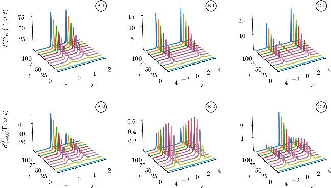
Figure 5. Time-dependent spectrum ${{ \mathcal S }}_{\gamma }({\rm{\Gamma }},\omega ;t)$ for the moving mirror. The upper row {A, B, C}. 1 are evolutions without decoherence, γ → ∞, whereas each column, A. 1, B. 2 and C. 3, represents linear, quadratic and linear-quadratic coupling, respectively. The same labeling system for the lower row. Here the relevant parameters are, Γ = 0.01, ωc = ωm = 1.0, gl = gq = 1.0. The initial state is one photonic excitation in the field, no phonons in the moving mirror, ∣ψ(0)⟩num = ∣1, 0⟩. |

Figure 6. Time-dependent spectrum ${{ \mathcal S }}_{\gamma }({\rm{\Gamma }},\omega ;t)$ for the moving mirror. The upper row {A, B, C}. 1 are evolutions without decoherence, γ → ∞, whereas each column, A. 1, B. 2 and C. 3, represents linear, quadratic and linear-quadratic coupling, respectively. The same labeling system for the lower row. Here the relevant parameters are Γ = 0.01, ωc = ωm = 1.0, gl = gq = 1.0. The initial state is a coherent state in the cavity field and in the moving mirror, ∣ψ(0)⟩coh = ∣2, 2⟩. |
Long-time limit
It is worth calculating the fate of the evolution as decoherence takes place. For this, we need to know the limits ${\mathrm{lim}}_{t\to \infty }{{\rm{e}}}^{-2{\rm{\Gamma }}t}| {{ \mathcal L }}_{k}^{(n)}(t){| }^{2}$, and ${\mathrm{lim}}_{t\to \infty }{{\rm{e}}}^{-2{\rm{\Gamma }}t}{{ \mathcal L }}_{j}^{(n)}(t){{ \mathcal L }}_{k}^{(n)}{(t)}^{* }$. Notice that these coefficients are defined in (23 ), the only terms that do not depend on Eγ(n) will be preserved, which exists in the last term of ${{ \mathcal L }}_{3}^{(n)}(t)$. This will lead us to the long-time spectrum of the form,
$\begin{eqnarray}\mathop{\mathrm{lim}}\limits_{t\to \infty }{{ \mathcal S }}^{(n,\beta )}({\rm{\Gamma }},\omega ;t)=\frac{2{\rm{\Gamma }}}{{{\rm{\Gamma }}}^{2}+{\omega }^{2}}\alpha {(n)}^{2}{{\rm{e}}}^{-2r(n)}.\end{eqnarray}$
This expression tells us that there is only one spectral peak at ω = 0, and that this peak only appears when there is either linear or linear-quadratic because when there is only quadratic coupling, α(n) = 0, meaning we obtain no spectral signature at final, as we can preview in panels (B. 2) of figures 3 and 4. Moreover, as we can see, the final spectral form does not depend on the initial state of the moving mirror, only on what we have in the cavity field at the beginning, ∣n⟩ or $| \tilde{\alpha }\rangle $.Let us dig in more in this regard. Suppose we want the steady-state of the system with initial condition ∣ψ(0⟩num = ∣n, m⟩, as it is in figure 3. The relation that can say something about the mechanical oscillator in a scenario of unchanged statistical properties, is equation (15 ). Here, we will ask for the value when the experiment reaches the end of the evolution at t → ∞, which is far beyond the point τc where the steady-state starts, but instead we obtain the value of the mean of phonons in this thermal state of the resonator. It results in the expression,
$\begin{eqnarray}\begin{array}{rcl} & & \mathop{\mathrm{lim}}\limits_{t\to \infty }\langle \psi (0)| {\hat{N}}_{\gamma }(t)| \psi (0)\rangle \\ & & \quad =m\frac{{\left({\omega }_{m}+2{g}_{q}n\right)}^{2}}{{\bar{\omega }}_{m}{(n)}^{2}}\\ & & \qquad +\left(\frac{1}{{\bar{\omega }}_{m}{(n)}^{2}}-\frac{{g}_{l}^{2}{n}^{2}{\omega }_{m}\left({\omega }_{m}-2{g}_{q}n\right)}{{\bar{\omega }}_{m}{(n)}^{4}}\right),\end{array}\end{eqnarray}$
contrasting with its associated spectral response $\begin{eqnarray*}{{ \mathcal S }}_{{\mathtt{lim}}}^{(n)}({\rm{\Gamma }},\omega )=\frac{2{\rm{\Gamma }}}{{{\rm{\Gamma }}}^{2}+{\omega }^{2}}\frac{{g}_{l}^{2}{n}^{2}{\omega }_{m}^{2}}{{\bar{\omega }}_{m}{(n)}^{4}}.\end{eqnarray*}$
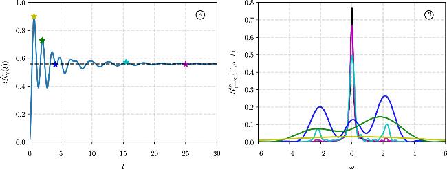
We can see that the steady-state of the mechanical resonator with this initial condition leads to a constant value proportional to combinations of power of ${\bar{\omega }}_{m}(n)$, which is also present in its spectral response, emerging as a Lorentzian peak modulated with the same proportional factor. In this sense, at thermal equilibrium, no energetic transitions are expected. In practice, with a dephasing factor γ below the hundredth, there is no need to expect infinitely long times for the steady-state, which also corresponds to a spectral peak dominating at ω = 0 for moderately long times.In figure 7, a comparative between the time evolution of the mean number of phonons for ∣ψ(0)⟩num = ∣1, 0⟩ is presented, and its corresponding spectral response for some selected times. In panel A, we observe the evolution of the mean phonon value $\langle {\hat{N}}_{\gamma }(t)\rangle $, and in panel B, we observe the formation of the spectrum ${{ \mathcal S }}_{\gamma }^{(n)}({\rm{\Gamma }},\omega ;t)$. The colors in the star marks in panel A, correspond to their respective spectrum in panel B, which was obtained by the relations in equations (15 ) and (24 ). Also note a faint black dashed line in panel A, which is the value of the steady-state given by equation (27 ), and its corresponding spectrum in panel B as a solid black line, given by equation (26 ). We can observe how the formation of the spectrum transits from an asymmetrical three-peak, to a single-peak in the long-time, centered at ω = 0. The asymmetry of the spectral peaks, as it was accused before, arises by the combination of linear and quadratic couplings, playing effects of squeezing, despite this, in the steady-state all non-linear effects are diminished due to the dephasing.
Figure 7. Time evolution and formation of the spectrum at some selected points, and in the long-time steady-state. Here the initial condition is ∣ψ(0)⟩ |
4. Conclusions
In this paper, the description of the dynamics and the spectral response in the linear-quadratic moving mirror-field system under pure dephasing decoherence is addressed. From the operational side, the full diagonalization using unitary transformations was done, since all the algebra generators closed under the Lie parenthesis, full analytical solutions can be obtained. The diagonalized Hamiltonian is composed of displaced and squeezed contributions, which leads to non-linear phenomena like revival-like of mean values when quadratic couplings are considered. The pure dephasing decoherence is introduced in the framework of the Milburn’s equation, which can be reduced to the Schrödinger–Heisenberg evolution when the decoherence rate is carried as an infinite limit. Finally, the time-dependent spectrum for the mirror response was obtained using the Eberly–Wódkiewicz non-stationary spectrum. Emphasis is given to the response of the mirror when there is a single photonic excitation, and no phonons. It is shown how the well-known results for the linear only coupling are modified by the inclusion of the second order term, the quadratic coupling, plus a view of the only quadratic is also given for the sake of comparison complement. From the dynamical standpoint, the evolution, considering decoherence is enabled, shows diminishing in the amplitudes of the mean values of phonons and the position quadrature. It is worth noticing that in a quadratic only coupling, it is equivalent to a mirror not moving at all. We can understand this due to the fact that the response of the mirror is to convert the photon to phonons due to radiation pressure, but the dephasing proportional to the decoherence rate γ damped this behavior, leading to a mean value in the phonons $\bar{N}$ and the quadrature $\bar{X}$ for a critical time tc where there is no more photon-phonon conversion. From the time-dependent spectral standpoint, the response of the mirror shows, for linear only coupling, that there are energetic transitions between the sidebands ω = 0, ωm, leading to just a single spectral peak at ω = 0, when the decoherence takes place. On the other hand, when there is quadratic only coupling, the unique chance the mirror has is to stop their movement, the transitions occur at $\omega =\pm \gamma \sin \frac{{\bar{\omega }}_{m}(n)}{\gamma }$, but disappear at long-time. Finally, when there are both couplings, linear and quadratic, it is expected to see transitions occurring as a triplet at $\omega =0,\pm \gamma \sin \frac{{\bar{\omega }}_{m}(n)}{\gamma }$, which carries the signatures of both contributions. Long-time limits were also presented, showing that only a spectral peak at ω0 is expected in linear and linear-quadratic couplings, and no spectral peak is expected in quadratic only coupling. The same analysis can be done when coherent states in both the field and the mirror, are prepared at the beginning. In this case, multipeaks are present, indicating simultaneous transitions. At the long-time limit, it is observed that same as the single photonic excitation, a spectral peak at ω = 0, or nothing at all, indicating the mirror stops its photon-phonon conversion.
Appendix. Diagonalization of the Hamiltonian
We now present the diagonalization of the Hamiltonian using unitary transformations. The Hamiltonian, as a reminder, is defined in full form by
$\begin{eqnarray}\hat{H}={\omega }_{c}\hat{n}+{\omega }_{m}\hat{N}-{g}_{l}\hat{n}\left({\hat{b}}^{\dagger }+\hat{b}\right)+{g}_{q}\hat{n}{\left({\hat{b}}^{\dagger }+\hat{b}\right)}^{2},\end{eqnarray}$
representing and optomechanical system whose mechanical frequency depending on the position is expanded up-to second order. Inspecting the interaction terms, with linear gl and quadratic gq coupling, we advert that geometrical unitary transformations must be needed: first, a one-mode squeezing, and second, a one-mode displacement in the mechanical operators.One-mode squeezing
The one-mode squeezing transformation is defined by the operator A1 ), resulting in
$\begin{eqnarray}\hat{S}(r(\hat{n}))={{\rm{e}}}^{\frac{1}{2}r(\hat{n})\left({\hat{b}{}^{\dagger }}^{2}-{\hat{b}}^{2}\right)},\quad {\hat{S}}^{\dagger }(r(\hat{n}))\equiv \hat{S}(-r(\hat{n})),\end{eqnarray}$
where $r(\hat{n})$ is a function depending on the number of photons, to be determined. The action of this transformation on the mirror operational basis is $\begin{eqnarray}\begin{array}{rcl}\hat{S}(r(\hat{n}))\,{\hat{b}}^{\dagger }\,{\hat{S}}^{\dagger }(r(\hat{n})) & = & {\hat{b}}^{\dagger }\cosh r(\hat{n})-\hat{b}\sinh r(\hat{n}),\\ \hat{S}(r(\hat{n}))\,\hat{b}\,{\hat{S}}^{\dagger }(r(\hat{n})) & = & \hat{b}\cosh r(\hat{n})-{\hat{b}}^{\dagger }\sinh r(\hat{n}).\end{array}\end{eqnarray}$
Knowing this, we can take the full transformation of the Hamiltonian ( $\begin{eqnarray}\begin{array}{rcl}\hat{S}(r)\hat{H}{\hat{S}}^{\dagger }(r) & = & {\omega }_{c}\hat{n}+{\omega }_{m}\hat{N}\cosh 2r-{g}_{l}\hat{n}\left({\hat{b}}^{\dagger }+\hat{b}\right){{\rm{e}}}^{-r}\\ & & -\,\frac{{\omega }_{m}}{2}\left({\hat{b}{}^{\dagger }}^{2}+{\hat{b}}^{2}\right)\sinh 2r\\ & & +\,{g}_{q}\hat{n}{\left({\hat{b}}^{\dagger }+\hat{b}\right)}^{2}{{\rm{e}}}^{-2r},\end{array}\end{eqnarray}$
which can be rearranged to highlight the quadratic terms we want to eliminate. The equation and the elimination conditions are, respectively, $\begin{eqnarray}\begin{array}{l}\left(-\frac{{\omega }_{m}}{2}\sinh 2r+{g}_{q}\hat{n}{{\rm{e}}}^{-2r}\right)\left({\hat{b}{}^{\dagger }}^{2}+{\hat{b}}^{2}\right)=0\\ \quad \Rightarrow r(\hat{n})=\frac{1}{4}\mathrm{ln}\left|1+\frac{4{g}_{q}\hat{n}}{{\omega }_{m}}\right|,\end{array}\end{eqnarray}$
where $r(\hat{n})$ is now identified as the squeezing parameter, preserving the unitariness of the transformation. The Hamiltonian after this one-mode squeezing operation takes the form $\begin{eqnarray}\begin{array}{rcl}{\hat{H}}_{{\mathtt{S}}} & = & {\omega }_{c}\hat{n}+{\bar{\omega }}_{m}(\hat{n})\hat{N}-{g}_{l}\hat{n}\left({\hat{b}}^{\dagger }+\hat{b}\right){{\rm{e}}}^{-r},\\ {\bar{\omega }}_{m}(\hat{n}) & = & \sqrt{{\omega }_{m}\left({\omega }_{m}+4{g}_{q}\hat{n}\right)},\end{array}\end{eqnarray}$
where the new frequency ${\bar{\omega }}_{m}(\hat{n})$ can be identified as a photon number-dependent frequency in the mechanical part influenced by the photonic counterpart.One-mode displacement
Because the one-mode squeezing transformation only deals with the quadratic part of the Hamiltonian (A1 ), the resulting Hamiltonian (A6 ) still has the lineal part damped with an exponential term in function of $r(\hat{n})$. A displacement transformation can be used, defined by
$\begin{eqnarray}\hat{D}(\alpha (\hat{n}))={{\rm{e}}}^{\alpha (\hat{n})\left({\hat{b}}^{\dagger }-\hat{b}\right)},\quad {\hat{D}}^{\dagger }(\alpha )\equiv \hat{D}(-\alpha ),\end{eqnarray}$
whose action on the mechanical operators is $\begin{eqnarray}\begin{array}{rcl}\hat{D}(\alpha (\hat{n})){\hat{b}}^{\dagger }{\hat{D}}^{\dagger }(\alpha (\hat{n})) & = & {\hat{b}}^{\dagger }-\alpha (\hat{n}),\\ \hat{D}(\alpha (\hat{n}))\hat{b}{\hat{D}}^{\dagger }(\alpha (\hat{n})) & = & \hat{b}-\alpha (\hat{n}),\end{array}\end{eqnarray}$
where the displacement argument observes realness, ${\rm{Im}}\left\{\alpha (\hat{n})\right\}=0$.Transforming the squeezed Hamiltonian (A6 ) using the rules (A8 ), we can identify the relations
$\begin{eqnarray}\begin{array}{l}\hat{D}(\alpha )\left({\omega }_{c}\hat{n}+{\bar{\omega }}_{m}(\hat{n})\hat{N}\right){\hat{D}}^{\dagger }(\alpha )={\omega }_{c}\hat{n}+{\bar{\omega }}_{m}(\hat{n})\hat{N}\\ \quad -{\bar{\omega }}_{m}(\hat{n})\alpha \left({\hat{b}}^{\dagger }+\hat{b}\right)+{\bar{\omega }}_{m}(\hat{n})| \alpha {| }^{2}={\hat{H}}_{{\mathtt{SD}}}\\ \quad \equiv {\omega }_{c}\hat{n}+{\bar{\omega }}_{m}(\hat{n})\hat{N}-{g}_{l}\hat{n}\left({\hat{b}}^{\dagger }+\hat{b}\right){{\rm{e}}}^{-r}\\ \quad \Rightarrow \alpha (\hat{n})=-\frac{{g}_{l}\hat{n}{{\rm{e}}}^{-r}}{{\bar{\omega }}_{m}(\hat{n})},\quad \therefore \,{\bar{\omega }}_{m}(\hat{n})| \alpha (\hat{n}){| }^{2}=\frac{{g}_{l}^{2}{\hat{n}}^{2}{{\rm{e}}}^{-2r}}{{\bar{\omega }}_{m}(\hat{n})},\end{array}\end{eqnarray}$
which define completely the transformation and the coefficient $\alpha (\hat{n})$. The full diagonal Hamiltonian now takes the form $\begin{eqnarray}{\hat{H}}_{{\mathtt{diag}}}={\omega }_{c}\hat{n}+{\bar{\omega }}_{m}(\hat{n})\hat{N}-\frac{{g}_{l}^{2}{\hat{n}}^{2}{{\rm{e}}}^{-2r}}{{\bar{\omega }}_{m}(\hat{n})},\end{eqnarray}$
where it can be identified as two harmonic oscillators, influenced by a Kerr-like term in the photonic field due to the presence of ${\hat{n}}^{2}$.Original representation
The diagonal representation in the original reference frame of the Hamiltonian (A1 ) is the successive transformation by $\hat{S}(r(\hat{n}))$ and $\hat{D}(\alpha (\hat{n}))$,
$\begin{eqnarray}\begin{array}{rcl}{\hat{H}}_{{\mathtt{diag}}} & \equiv & \hat{D}(\alpha (\hat{n}))\hat{S}(r(\hat{n}))\hat{H}{\hat{S}}^{\dagger }(r(\hat{n})){\hat{D}}^{\dagger }(\alpha (\hat{n}))\\ & \Rightarrow & \hat{H}={\hat{S}}^{\dagger }(r(\hat{n}))\hat{D}(\alpha (\hat{n}))\,{\hat{H}}_{{\mathtt{diag}}}\,\hat{D}(\alpha (\hat{n}))\hat{S}(r(\hat{n})).\end{array}\end{eqnarray}$
Heisenberg representation and expectation values
Relation (A11 ) defines the evolution operator of the full system
$\begin{eqnarray}\hat{{ \mathcal U }}(t)={\hat{S}}^{\dagger }(r)\hat{D}(\alpha ){{\rm{e}}}^{-{\rm{i}}t{\hat{H}}_{{\mathtt{diag}}}}\hat{D}(\alpha )\hat{S}(r),\end{eqnarray}$
that is used to calculate the time evolution of operators. The Heisenberg representation of the mechanical operators is obtained as $\begin{eqnarray}\begin{array}{rcl}{\hat{U}}^{\dagger }(t){\hat{b}}^{\dagger }\hat{U}(t) & = & {\xi }_{1}(t){\hat{b}}^{\dagger }+{\xi }_{2}(t)\hat{b}+{\xi }_{3}(t),\\ {\hat{U}}^{\dagger }(t)\hat{b}\,\hat{U}(t) & = & {\xi }_{1}^{* }(t)\hat{b}+{\xi }_{2}^{* }(t){\hat{b}}^{\dagger }+{\xi }_{3}^{* }(t),\end{array}\end{eqnarray}$
where the companion time-dependent coefficients are $\begin{eqnarray}\begin{array}{c}{\xi }_{1}(t)\,=\,\cos \left({\bar{\omega }}_{m}(\hat{n})t\right)\\ +\,{\rm{i}}\cosh \left(2r\right)\sin \left({\bar{\omega }}_{m}(\hat{n})t\right),\\ {\xi }_{2}(t)\,=\,{\rm{i}}\,\sinh \left(2r\right)\sin \left({\bar{\omega }}_{m}(\hat{n})t\right),\\ {\xi }_{3}(t)\,=\,\alpha \left[\left(1-{{\rm{e}}}^{{\rm{i}}{\bar{\omega }}_{m}(\hat{n})t}\right)\cosh \left(r\right)\right.\\ \left.+\,(1-{{\rm{e}}}^{-{\rm{i}}{\bar{\omega }}_{m}(\hat{n})t})\sinh \left(r\right)\right],\end{array}\end{eqnarray}$
determining completely the dynamics of the time evolution.