


1. Introduction
The quantum parameter estimation theory is a fundamental tool for understanding the quantum limit of precision in estimating unknown parameters [1–7]. In cases where the quantum system depends on multiple parameters, the quantum Fisher information (QFI) matrix can be used to analyze the quantum limit of precision in parameter estimation [8]. However, quantum multiparameter estimation is more complicated than single-parameter estimation, not only because of the incompatibility problem [9, 10] but also because of the diversity of parametrization. Even when focusing on a single parameter of interest, the presence of additional parameters may influence the overall precision of the estimation process. To reveal the practical quantum limits on parameter estimation, quantum multiparameter estimation theory should be properly used.
The Mach–Zehnder interferometer (MZI) is a fundamental optical device that plays a crucial role in studying the coherence properties of light fields [11]. A key parameter in this interferometer is the relative phase difference between its two arms, which has been the focus of significant research efforts [12]. The QFI approach has been widely utilized to optimize the MZI for various input states and to explore the quantum limit of phase estimation [13–15]. Notably, Jarzyna and Demkowicz-Dobrzański in [16] pointed out the potential flaws in the simplified models of MZI when using the QFI to reveal the fundamental limit of phase estimation, suggesting that these models might not fully reflect the practical limits of phase estimation.
In this paper, we revisit the quantum parameter estimation approach for the MZI. We will analyze different models for estimating the relative phase shift in the MZI and show how to understand the applicabilities of these models through the quantum multiparameter estimation theory. We will show that the QFI matrix, which is the core quantity in the quantum multiparameter estimation theory, contains enough information about the precision of phase estimation in the MZI. Even when we are only interested in the relative phase shift between the two arms, the QFI matrix should be used to analyze the precision of the phase estimation. The QFI matrix can be applied in two ways: (i) to analyze the estimation precision of the relative phase shift in the presence of nuisance parameters and (ii) to analyze the precision of phase estimation in the presence of prior constraints on the parameters. Several single-parameter models for estimating the relative phase shift in the MZI should be interpreted as the QFI about the relative phase shift in the presence of proper constraints; otherwise, the QFI may be overoptimistic. Moreover, we will specifically examine the QFI approach for the MZI with an input state composed of a displaced squeezed vacuum state and a coherent state.
This paper is organized as follows. In section 2 , we give a general analysis of phase estimation in an MZI. In section 3 , we study the phase estimation in an MZI with a displaced squeezed vacuum state and a coherent state as input. We summarize our work in section 4 and give the details of some calculations in the appendix .
2. Phase estimation in the MZI
Let us denote by a1 and a2 the annihilation operators of the two input modes of an MZI. The input state is a product state ∣ψ0⟩ = ∣ψ1⟩ ⨂ ∣ψ2⟩. It first evolves through a unitary process U1 and then passes through a channel with two arms. The upper and lower arms cause phase shifts φ1 and φ2, respectively, as shown in figure 1(a). The corresponding unitary transformation is given by
$\begin{eqnarray}{U}_{{\varphi }_{1}{\varphi }_{2}}=\exp (-{\rm{i}}{\varphi }_{1}{a}_{1}^{\dagger }{a}_{1}-{\rm{i}}{\varphi }_{2}{a}_{2}^{\dagger }{a}_{2}).\end{eqnarray}$
For an optical interferometer, the quantum state typically goes through another unitary process U2, e.g., a beam splitter, before the final measurement. The unitary operator U1 and U2 are independent of the phase parameters φ1 and φ2. The output state ∣ψ⟩ is given by $| \psi \rangle ={U}_{2}{U}_{{\varphi }_{1}{\varphi }_{2}}{U}_{1}| {\psi }_{0}\rangle $.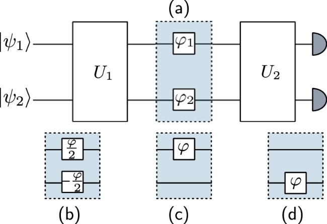
Figure 1. Different parametrization models of the MZI. (a) Two-parameter estimation model. (b)–(d) Various single-parameter estimation models. |
The relative phase shift φ1 − φ2 between the two arms is usually the parameter of interest. Therefore, it will be convenient to use φ± := φ1 ± φ2 as the independent parameters instead of the original ones φ1 and φ2. As the photon number operator $N:= {a}_{1}^{\dagger }{a}_{1}+{a}_{2}^{\dagger }{a}_{2}$ commute with ${a}_{1}^{\dagger }{a}_{1}-{a}_{2}^{\dagger }{a}_{2}$, the unitary operator ${U}_{{\varphi }_{1}{\varphi }_{2}}$ can be decomposed into
$\begin{eqnarray}{U}_{{\varphi }_{1}{\varphi }_{2}}=\exp \left(-\frac{{\rm{i}}{\varphi }_{+}}{2}N\right)\exp \left[-\frac{{\rm{i}}{\varphi }_{-}}{2}({a}_{1}^{\dagger }{a}_{1}-{a}_{2}^{\dagger }{a}_{2})\right].\end{eqnarray}$
According to the quantum parameter estimation theory, we can calculate the QFI matrix ${ \mathcal F }$ about φ± to analyze the precision of the phase estimation. For pure states, the QFI matrix ${ \mathcal F }$ can be calculated as $\begin{eqnarray}{{ \mathcal F }}_{{jk}}=4{\rm{Re}}(\langle {{\rm{\partial }}}_{j}\psi \,{{\rm{\partial }}}_{k}\psi \rangle -\langle {{\rm{\partial }}}_{j}\psi |\psi \rangle \langle \psi |{{\rm{\partial }}}_{k}\psi \rangle ),\end{eqnarray}$
with ∂1 = ∂/∂φ+ and ∂2 = ∂/∂φ−. The inverse of the QFI matrix ${{ \mathcal F }}^{-1}$ bounds the covariance matrix ${ \mathcal E }$ of any unbiased estimator [1, 2] as $\begin{eqnarray}{ \mathcal E }\geqslant {\nu }^{-1}{{ \mathcal F }}^{-1},\end{eqnarray}$
where ν is the number of repetitions of the experiment.When focusing on the relative phase shift φ−, it is tempting to use quantum single-parameter estimation theory for precision analysis. The analysis often employs various simplified models for estimating the relative phase shift φ− in an MZI, as demonstrated in figures 1(b)-(d). However, such approaches must be grounded in robust theoretical frameworks and carefully examined to avoid being overoptimistic about the estimation precision. In what follows, we shall investigate several existing single-parameter estimation models for the MZI and show how to understand their applicabilities by quantum multiparameter estimation theory.
The typical theoretical models of estimating the relative phase shift are illustrated in figure 1. With a slight abuse of notation, we use φ instead of φ− to simplify the notation, as we focus on the relative phase shift. For the model shown in figure 1(a), the value of the common phase shift φ+ is unknown and not of our interest, that is to say, φ+ is a nuisance parameter [17]. The model shown in figure 1(b) assumes that the phase shifts in the two arms are equal in magnitude but opposite in sign, i.e., φ1 = φ/2 and φ2 = − φ/2. In this model, any common phase shift φ+ is considered irrelevant and is set to zero. This approach is widely used in optical interferometry [12, 18], especially when the observable finally measured commutes with the total photon number operator N. The models shown in figures 1(c) and (d) assume that the phase shift occurs only in one arm of the interferometer, while the other arm has no phase shift.
The QFIs about the relative phase shift for these four models are given by 3 ), meaning that the two-parameter estimation model shown in figure 1(a) is the most general scenario for estimating the relative phase shift in an MZI and the two-parameter QFI matrix contains sufficient information about the estimation precision.
$\begin{eqnarray}{{ \mathcal F }}_{\varphi }^{(a)}={{ \mathcal F }}_{22}-{{ \mathcal F }}_{12}^{2}/{{ \mathcal F }}_{11},\end{eqnarray}$
$\begin{eqnarray}{{ \mathcal F }}_{\varphi }^{(b)}={{ \mathcal F }}_{22},\end{eqnarray}$
$\begin{eqnarray}{{ \mathcal F }}_{\varphi }^{(c)}={{ \mathcal F }}_{11}+2{{ \mathcal F }}_{12}+{{ \mathcal F }}_{22},\end{eqnarray}$
$\begin{eqnarray}{{ \mathcal F }}_{\varphi }^{(d)}={{ \mathcal F }}_{11}-2{{ \mathcal F }}_{12}+{{ \mathcal F }}_{22}.\end{eqnarray}$
All the above results are expressed in terms of the QFI matrix elements ${{ \mathcal F }}_{jk}$ defined in equation (Note that ${{ \mathcal F }}_{\varphi }^{(a)}$ is equal to $1/{({{ \mathcal F }}^{-1})}_{22}$ due to the explicit form of the inverse matrix of any 2 × 2 matrix. It can be seen from equation (4 ) that the variance of any unbiased estimator $\hat{\varphi }$ must obey ${\rm{Var}}(\hat{\varphi })\geqslant {({{ \mathcal F }}^{-1})}_{22}/\nu =1/(\nu {{ \mathcal F }}_{\varphi }^{(a)})$. In other words, ${{ \mathcal F }}_{\varphi }^{(a)}$ is the QFI about the relative phase shift in the presence of nuisance parameter φ+.
The quantities ${{ \mathcal F }}_{\varphi }^{(b)}$, ${{ \mathcal F }}_{\varphi }^{(c)}$, and ${{ \mathcal F }}_{\varphi }^{(d)}$ are the QFIs for single-parameter model of estimating the relative phase shift. These QFIs were studied in the prior work, e.g., see [16, 19]. Here, we show that they can be obtained from the two-parameter QFI matrix ${ \mathcal F }$ by setting proper constraints on the parameter space (φ1, φ2). Without loss of generality, assume there is a constraint f(φ−, φ+) = 0 on the unknown parameters. The constraint reduces the dimension of the parameter space. As shown in figure 2, the constraint f(φ−, φ+) = 0 can be viewed as a curve in the parameter space. To reduce the model from two-parameter estimation to single-parameter estimation, we can choose (f, g) as the two new parameters, where g is another independent function of φ+ and φ−. The QFI matrix in the new basis $\tilde{\theta }=(f,g)$ is given by
$\begin{eqnarray}\tilde{{ \mathcal F }}={{ \mathcal J }}^{{\mathsf{T}}}{ \mathcal F }{ \mathcal J },\end{eqnarray}$
where $\begin{eqnarray}{ \mathcal J }=\left(\begin{array}{l}\partial {\varphi }_{+}/\partial f,\partial {\varphi }_{+}/\partial g\\ \partial {\varphi }_{-}/\partial f,\partial {\varphi }_{-}/\partial g\end{array}\right)\end{eqnarray}$
is the Jacobian matrix of the parameter transform. The QFI about the parameter g with the constraint f = c, where c is any constant, is given by ${\tilde{{ \mathcal F }}}_{22}$ at f = c.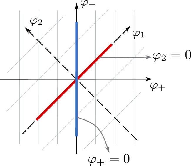
Figure 2. Various constraints on the parameter space. |
From the above approach to reduce the model from two-parameter estimation to single-parameter estimation, we can see that ${{ \mathcal F }}_{\varphi }^{(b)}$ is the QFI about the relative phase shift in the presence of the constraint φ+ = c. To derive ${{ \mathcal F }}_{\varphi }^{(c)}$ and ${{ \mathcal F }}_{\varphi }^{(d)}$ from the two-parameter QFI matrix ${ \mathcal F }$, we need to transform the QFI matrix from the basis (φ+, φ−) to the parameter basis (φ1, φ2) according to equation (9 ), that is,
$\begin{eqnarray}\tilde{{ \mathcal F }}=\left(\begin{array}{l}{{ \mathcal F }}_{11}+2{{ \mathcal F }}_{12}+{{ \mathcal F }}_{22}{{ \mathcal F }}_{11}-{{ \mathcal F }}_{22}\\ {{ \mathcal F }}_{11}-{{ \mathcal F }}_{22}{{ \mathcal F }}_{11}-2{{ \mathcal F }}_{12}+{{ \mathcal F }}_{22}\end{array}\right).\end{eqnarray}$
Therefore, ${{ \mathcal F }}_{\varphi }^{(c)}$ is given by ${\tilde{{ \mathcal F }}}_{11}$ at φ2 = c and ${{ \mathcal F }}_{\varphi }^{(d)}$ is given by ${\tilde{{ \mathcal F }}}_{22}$ at φ1 = c.The above analysis suggests that, in order to make the single-parameter QFIs about the relative phase shift meaningful, the corresponding constraints must be ensured in the experiment. Otherwise, the single-parameter QFIs might be overoptimistic for the quantum limit of estimation precision. In many realistic scenarios, e.g., gravitational wave detection [20], the MZI is operated at an adjustable working phase point and the parameter to be estimated is a tiny phase perturbation. The model in figures 1(b)–(d) stand for different sensing mechanisms in the MZI. They can be understood as different curves determined by corresponding constraint in the parameter space, as shown in figure 2.
Note that ${{ \mathcal F }}_{\varphi }^{(c)}$ is greater than ${{ \mathcal F }}_{22}$ when ${{ \mathcal F }}_{12}\geqslant 0$. The reason being that not only does the constraint bring in the prior information about the values of parameters, but also that there is a scaling operation in the parameter transform from (φ+, φ−) to (φ1, φ2). In other words, the determinant of the Jacobian matrix ${ \mathcal J }$ is not equal to 1 so that the determinant of the QFI matrix $\tilde{{ \mathcal F }}$ is not equal to the determinant of the original QFI matrix ${ \mathcal F }$. This fact should be taken into account when comparing the QFIs in different models.
From the above analysis, it can be seen that the unconstrained scheme as figure 1(a) shown is suitable when the common phase shift is treated as a nuisance parameter. Other single-parameter models are not equivalent and might underestimate the Cramér–Rao bound on the estimation error of the relative phase shift in the absence of proper constraints. When there is a constraint on the parameter space, these single-parameter models can be used to analyze the achievable limit of the estimation precision. We will use these QFIs to analyze the MZI with the displaced squeezed vacuum state and the coherent state as input in next section.
3. Displaced squeezed vacuum state plus coherent state as input
We now consider an MZI that takes the product state of a displaced squeezed state and a coherent state as the input. The classical Fisher information for the photon counting of the two output modes under this model is given in [21]. Here we calculate the QFIs to analyze the fundamental limit of precision in estimating the phase difference between the two arms. The input state is expressed as
$\begin{eqnarray}| {\psi }_{0}\rangle =| {\alpha }_{1},r\rangle \otimes | {\alpha }_{2}\rangle ,\end{eqnarray}$
where ∣α1, r⟩ is a displaced squeezed vacuum state with a zero squeeze angle, i.e., ∣α1, r⟩ = D(α1)S(r)∣0⟩ with $D({\alpha }_{1})={{\rm{e}}}^{{\alpha }_{1}{a}^{\dagger }-{\alpha }_{1}^{* }a}$ and $S(r)={{\rm{e}}}^{r({a}^{2}-{a}^{\dagger 2})/2}$ being the displacement and squeeze operators, respectively, and ∣α2⟩ is a coherent state. We henceforth assume that the squeeze parameter r ≥ 0. The two beam splitters are both 50:50 and the corresponding unitary transformations are given by ${U}_{\,\rm{BS}\,}={{\rm{e}}}^{-{\rm{i}}\pi ({a}_{1}^{\dagger }{a}_{2}+{a}_{2}^{\dagger }{a}_{1})/4}$ and ${U}_{{\rm{BS}}}^{\dagger }$. After the first beam splitter, the state evolves through a channel with phase shifts φ1 and φ2 in the upper and lower arms, respectively, as shown in figure 3(a). After the second beam splitter, the output state is given by $| \psi \rangle ={U}_{\rm{BS}\,}^{\dagger }{U}_{{\varphi }_{1}{\varphi }_{2}}{U}_{\,\rm{BS}}| {\psi }_{0}\rangle $, for which we can calculate the QFI matrix to analyze the precision of the phase estimation.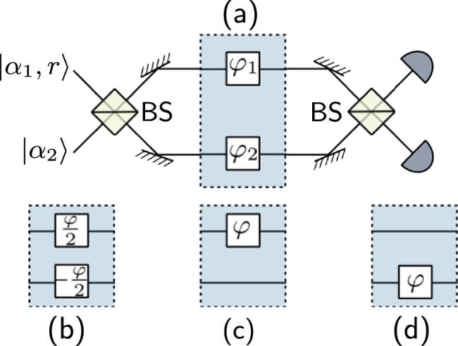
Figure 3. Mach–Zehnder interferometer with a displaced squeezed state and a coherent state as input. |
The MZI has the SU(2) mathematical structure and can be conveniently described by the SU(2) generators [18], 3 ), we obtain the elements of the QFI matrix about the parameters φ+ and φ− as appendix .
$\begin{eqnarray}{J}_{1}=\frac{1}{2}\left({a}_{1}^{\dagger }{a}_{2}+{a}_{2}^{\dagger }{a}_{1}\right),\end{eqnarray}$
$\begin{eqnarray}{J}_{2}=\frac{1}{2{\rm{i}}}\left({a}_{1}^{\dagger }{a}_{2}-{a}_{2}^{\dagger }{a}_{1}\right),\end{eqnarray}$
$\begin{eqnarray}{J}_{3}=\frac{1}{2}\left({a}_{1}^{\dagger }{a}_{1}-{a}_{2}^{\dagger }{a}_{2}\right),\end{eqnarray}$
as well as the total number operator $N={a}_{1}^{\dagger }{a}_{1}+{a}_{2}^{\dagger }{a}_{2}$. Note that Ji satisfies the SU(2) commutation relation [Ji, Jj] = iεijkJk and N commutes with all Ji. With these operators, the total unitary transformation can be expressed as $\begin{eqnarray}{U}_{\rm{BS}\,}^{\dagger }{U}_{{\varphi }_{1}{\varphi }_{2}}{U}_{\,\rm{BS}}=\exp \left(-\frac{{\rm{i}}}{2}{\varphi }_{+}N\right)\exp (-{\rm{i}}{\varphi }_{-}{J}_{2}),\end{eqnarray}$
where φ± = φ1 ± φ2. Using equation ( $\begin{eqnarray}\begin{array}{rcl}{{ \mathcal F }}_{11} & = & \langle {N}^{2}\rangle -{\langle N\rangle }^{2},\\ {{ \mathcal F }}_{12} & = & 2\langle N{J}_{2}\rangle -2\langle N\rangle \langle {J}_{2}\rangle ,\\ {{ \mathcal F }}_{22} & = & 4{\langle {J}_{2}\rangle }^{2}-4{\langle {J}_{2}\rangle }^{2},\end{array}\end{eqnarray}$
and ${{ \mathcal F }}_{21}={{ \mathcal F }}_{12}$, where the expectation values are taken with respect to the input state ∣ψ0⟩. Substituting the concrete state ∣ψ0⟩ = ∣α1, r⟩ ⨂ ∣α2⟩, the final result is $\begin{eqnarray}\begin{array}{rcl}{{ \mathcal F }}_{11} & = & | {\alpha }_{2}{| }^{2}+\frac{{\sinh }^{2}2r}{2}+{{\rm{\Theta }}}_{1},\\ {{ \mathcal F }}_{22} & = & | {\alpha }_{1}{| }^{2}+{\sinh }^{2}r+{{\rm{\Theta }}}_{2},\\ {{ \mathcal F }}_{12} & = & -{\rm{Im}}\left({\alpha }_{1}{\alpha }_{2}\right)\sinh 2r+2{\rm{Im}}\left({\alpha }_{1}^{* }{\alpha }_{2}\right){\cosh }^{2}r,\end{array}\end{eqnarray}$
where $\begin{eqnarray}{{\rm{\Theta }}}_{1}={({\rm{Re}}{\alpha }_{1})}^{2}{{\rm{e}}}^{-2r}+{({\rm{Im}}{\alpha }_{1})}^{2}{{\rm{e}}}^{2r},\end{eqnarray}$
$\begin{eqnarray}{{\rm{\Theta }}}_{2}={({\rm{Im}}{\alpha }_{2})}^{2}{{\rm{e}}}^{-2r}+{({\rm{Re}}{\alpha }_{2})}^{2}{{\rm{e}}}^{2r}.\end{eqnarray}$
We give the detailed calculation of the QFI matrix in the We take n1 = ∣α1∣2, n2 = ∣α2∣2, and the squeeze parameter r as the measures on the resources used in the MZI. In what follows, we will study the optimization of different scenarios over the arguments of α1 and α2.
If the common phase shift φ+ is treated as a nuisance parameter, the QFI about φ− is given by ${{ \mathcal F }}_{\varphi }^{(a)}\,={{ \mathcal F }}_{22}-{{ \mathcal F }}_{12}^{2}/{{ \mathcal F }}_{11}$, which is smaller than ${{ \mathcal F }}_{22}$ unless ${{ \mathcal F }}_{12}=0$. For fixed n1, n2, and r, ${{ \mathcal F }}_{\varphi }^{(a)}$ attains its maximum 21 ), when α2 is real.
$\begin{eqnarray}{{ \mathcal F }}_{\varphi }^{(a)}={n}_{1}+{\sinh }^{2}r+{n}_{2}{{\rm{e}}}^{2r},\end{eqnarray}$
when α1 and α2 are both real numbers. If the common phase shift is treated as a constraint, the QFI ${{ \mathcal F }}_{\varphi }^{(b)}$ about φ− for fixed n1, n2, and r attains its maximum, which is the same as equation (When the constraint comes to φ2 = c as shown in figure 3(c), the QFI about φ is given by ${{ \mathcal F }}_{\varphi }^{(c)}={{ \mathcal F }}_{11}\,+2{{ \mathcal F }}_{12}+{{ \mathcal F }}_{22}$ according to equation (7 ). We found that if ${\rm{Re}}{\alpha }_{1}=-{\rm{Im}}{\alpha }_{2}$ and ${\rm{Im}}{\alpha }_{1}={\rm{Re}}{\alpha }_{2}$ are satisfied, ${{ \mathcal F }}_{\varphi }^{(c)}$ has a concise result as follows
$\begin{eqnarray}{{ \mathcal F }}_{\varphi }^{(c)}=(2+\cosh 2r){\sinh }^{2}r.\end{eqnarray}$
Note that the mean photon numbers of squeezed vacuum state is ${n}_{s}={\sinh }^{2}r$. Therefore, the expression of QFI is ${{ \mathcal F }}_{\varphi }^{(c)}=(3+2{n}_{s}){n}_{s}$. Meanwhile, the variance is bounded from below by $\begin{eqnarray}{\rm{Var}}(\hat{\varphi })\geqslant \frac{1}{{{ \mathcal F }}_{\varphi }^{(c)}}=\frac{1}{(3+2{n}_{s}){n}_{s}}.\end{eqnarray}$
Similarly, setting ${\rm{Re}}{\alpha }_{1}={\rm{Im}}{\alpha }_{2}$, ${\rm{Im}}{\alpha }_{1}=-{\rm{Re}}{\alpha }_{2}$, the QFI also will be ${{ \mathcal F }}_{\varphi }^{(d)}=(2+\cosh 2r){\sinh }^{2}r$, and there will be the same result as ${{ \mathcal F }}_{\varphi }^{(c)}$.4. Conclusion
In this work, we have analyzed different theoretical models for estimating the relative phase shift in the arms of an MZI. We pointed out that there are two type of models for estimating the relative phase shift in the MZI: the nuisance parameter model and the constrained model. The nuisance parameter model treats the common phase shift as a nuisance parameter and the relative phase shift as the parameter to be estimated. The constrained model sets a constraint on the parameter space to reduce the model from two-parameter estimation to single-parameter estimation. The selection of the model depends on the experimental setup and the prior information about the parameters. If the constrained model is used but the constraint is not satisfied in the experiment, the QFI about the relative phase shift might be overoptimistic. Moreover, we have shown that the QFIs in the constrained model can be obtained from the two-parameter QFI matrix by imposing proper constraints on the parameter space, so for theoretical work the two-parameter QFI matrix is sufficient to analyze the precision of the phase estimation. Our work provides a unified framework to analyze the precision of phase estimation in the MZI and highlights the importance of the constraints in the parameter space.