


1. Introduction
In quantum computation and quantum information, there are two widely used paradigms: the first involves discrete-variable systems such as qubits, while the second involves continuous-variable systems such as quantum oscillators (bosonic systems). In both paradigms, quantum gates (unitary operators) are analogous to classical logic gates but operate on quantum states. Quantum gates manipulate the input quantum states to perform specific quantum operations, which may offer quantum computational advantages over classical computation [1].
In the stabilizer formalism of discrete-variable quantum computation, quantum circuits with Clifford gates, stabilizer states and Pauli measurements can be efficiently simulated by classical computers, as ensured by the Gottesman–Knill theorem [1–3]. To realize genuine quantum computation, it is necessary to invoke non-stabilizer states or non-Clifford gates, which can generate magic resources from stabilizer states [4–9]. In a qubit or qutrit system, the well-known T-gates [1, 5]
$\begin{eqnarray*}{T}_{{\rm{qubit}}}=\left(\begin{array}{cc}1 & 0\\ 0 & {{\rm{e}}}^{{\rm{i}}\pi /4}\end{array}\right),\quad {T}_{{\rm{qutrit}}}=\left(\begin{array}{ccc}1 & 0 & 0\\ 0 & {{\rm{e}}}^{{\rm{i}}2\pi /9} & 0\\ 0 & 0 & {{\rm{e}}}^{-{\rm{i}}2\pi /9}\end{array}\right)\end{eqnarray*}$
are standard non-Clifford gates for implementing universal quantum computation. Indeed, the framework of ‘Clifford+T’, which involves the combination of Clifford gates and T-gates, has been widely used in designing and analyzing quantum circuits [10–15]. Moreover, the T-count (the number of quantum T-gates in a quantum circuit) has become a benchmark for describing the complexity of a quantum circuit [16–18].While qubit systems are widely used in quantum information processing, qudits do offer some advantage and convenience in certain contexts. Many practical quantum systems, including spin systems and multi-level atoms, are described by finite-dimensional Hilbert spaces where the dimensions may be arbitrary [19–22]. To exploit such systems for quantum computation, it is necessary to construct high-dimensional analogies of T-gates in arbitrary dimensions. In a remarkable piece of work, Howard and Vala introduced qudit versions of T-gates for prime dimensional systems [5], which have important applications in fault-tolerant quantum computation [20–28].
Differently from the discrete-variable scenario, the continuous-variable quantum information based on systems such as optical devices, superconducting circuits, cavity optomechanics, etc., provides another powerful and convenient paradigm [29–43]. Gaussian states (including coherent states, squeezed coherent states, and thermal states), which capture many amenable properties of continuous-variable systems, play an important role in continuous-variable quantum information [31, 32]. Non-Gaussianity, on the other hand, can be viewed as quantum resources in quantum information processing [44–52]. Gaussian gates are associated with Gaussian transformations which preserve the Gaussian nature of quantum states, i.e., send Gaussian states to Gaussian states. Lloyd highlighted that the set of Gaussian gates is inadequate for constructing arbitrary polynomial Hamiltonian transformations and pointed out that the addition of any single non-Gaussian gate is sufficient for achieving universal quantum computation [29]. Cubic phase gates, as the simplest non-Gaussian gates, have been widely employed in certain continuous-variable quantum protocols [53–58]. In [33, 53], a universal gate set for continuous-variable systems is given by
$\begin{eqnarray*}\{{{\rm{e}}}^{{\rm{i}}p{ \mathcal Q }}\,:\,p\in {\mathbb{R}}\}\cup \{{{\rm{e}}}^{{\rm{i}}\kappa {{ \mathcal Q }}^{2}/2}:\,\kappa \in {\mathbb{R}}\}\cup \{{{\rm{e}}}^{{\rm{i}}\pi ({{ \mathcal Q }}^{2}+{{ \mathcal P }}^{2})/4}\}\cup \{{{\rm{e}}}^{{\rm{i}}\gamma {{ \mathcal Q }}^{3}}\},\end{eqnarray*}$
where the constant $\gamma \in {\mathbb{R}}\backslash \{0\}$, and ${ \mathcal Q }$ and ${ \mathcal P }$ are the canonical position and momentum observables of an oscillator (single-mode bosonic system).Apart from the Howard–Vala T-gates in prime dimensions [5], we are still lacking T-gates in arbitrary dimensions, and it is desirable to construct such gates, generalizing that of Howard and Vala [5]. By exploiting the analogies between Clifford/non-Clifford gates in discrete-variable systems and Gaussian/non-Gaussian gates in continuous-variable systems, we derive general T-gates from cubic phase gates in continuous-variable systems via the Gottesman–Kitaev–Preskill (GKP) encoding, which encodes discrete qudits into continuous-variable systems involving oscillators and serves as a natural bridge connecting discrete and continuous worlds [59]. We further apply the obtained T-gates to construct some interesting frames including certain MUBs (mutually unbiased bases).
The work is structured as follows. In section 2 , we recall some basic features of both discrete- and continuous-variable quantum systems. In particular, for discrete-variable systems, we recall the discrete Heisenberg–Weyl group and the associated Clifford group. For continuous-variable systems, we recall continuous Heisenberg–Weyl group and Gaussian gates. We also review GKP encoding from both intuitive and rigorous perspectives. In section 3 , we first recall the T-gates in prime dimensional systems. Then we employ the GKP encoding to construct the T-gates (in arbitrary dimensional systems) from the conventional cubic phase gates in continuous-variable systems. This is achieved by ensuring the preservation of the GKP code space, from which certain parameters of the cubic phase gates are determined. This allows us to derive general T-gates as discrete counterparts of the continuous-variable cubic phase gates. We reveal some basic properties of the introduced T-gates. We further compare the Gaussian hierarchy in continuous-variable systems and the Clifford hierarchy in discrete-variable systems. In section 4 , we make a comparison between our T-gates and the Howard–Vala T-gates, and reveal their relationships. In section 5 , as an application of the T-gates, we construct some equidistributed n-angular frames including some MUBs as special instances. Finally, we conclude with a summary and discussion in section 6 .
2. Preliminaries
In this section, we recall the Clifford gates in discrete-variable systems, and their continuous analogies, the Gaussian gates, in continuous-variable systems. We also review basic aspects of GKP encoding, which will play a crucial role in our approach to T-gates.
2.1. Clifford gates in discrete-variable systems
Let ${{\mathbb{Z}}}_{d}=\{0,1,\cdots \,,\,d-1\}$ be the ring of integers modulo d, and ${{\mathbb{C}}}^{d}={L}^{2}({{\mathbb{Z}}}_{d})$ be the d-dimensional complex Hilbert space with computational basis $\{| j\rangle :j\in {{\mathbb{Z}}}_{d}\}.$ Let
$\begin{eqnarray}X=\displaystyle \sum _{j=0}^{d-1}|j+1\rangle \langle j|,\,Z=\displaystyle \sum _{j=0}^{d-1}{\omega }^{j}|j\rangle \langle j|,\,\omega ={{\rm{e}}}^{{\rm{i}}2\pi /d},\end{eqnarray}$
which satisfy the commutation relation ZX = ωXZ. These two unitary operators are introduced by Schwinger in his seminal study of unitary operator bases [60], and are fundamental ingredients of discrete-variable quantum theory. The discrete Heisenberg–Weyl (generalized Pauli) group ${\mathscr{P}}$ of the d-dimensional system ${{\mathbb{C}}}^{d}$ is defined as [61] $\begin{eqnarray*}{\mathscr{P}}=\{{\tau }^{c}{D}_{k,l}\,:c\in {\mathbb{Z}},k,l\in {{\mathbb{Z}}}_{d}\}\end{eqnarray*}$
with $\begin{eqnarray*}{D}_{k,l}={\tau }^{kl}{X}^{k}{Z}^{l},\qquad \tau =-{{\rm{e}}}^{{\rm{i}}\pi /d}\end{eqnarray*}$
being the discrete Heisenberg–Weyl operators (displacement operators) [61]. Moreover, $\{\frac{1}{\sqrt{d}}{D}_{k,l}:k,l\in {{\mathbb{Z}}}_{d}\}$ constitutes an orthonormal basis for the d2-dimensional operator space of all linear operators (matrices) on ${{\mathbb{C}}}^{d}$ endowed with the Hilbert–Schmidt inner product $\langle A| B\rangle ={\rm{tr}}{A}^{\dagger }B.$As the normalizer of the discrete Heisenberg–Weyl group in the unitary group ${\mathscr{U}}$ of ${{\mathbb{C}}}^{d}$, the Clifford group [61]
$\begin{eqnarray*}{\mathscr{C}}=\{U\in {\mathscr{U}}\,:U{\mathscr{P}}{U}^{\dagger }={\mathscr{P}}\}\end{eqnarray*}$
consists of those unitary operators on ${{\mathbb{C}}}^{d}$ mapping the discrete Heisenberg–Weyl group into itself under unitary conjugation. According to the definition of the Clifford group, for any $U\in {\mathscr{C}}$ and any ${D}_{k,l}\in {\mathscr{P}}$, we have $U{D}_{k,l}{U}^{\dagger }\in {\mathscr{P}}$, which means that there exists a liner transformation ${{\rm{\Gamma }}}_{U}\,:{{\mathbb{Z}}}_{d}\times {{\mathbb{Z}}}_{d}\to {{\mathbb{Z}}}_{d}\times {{\mathbb{Z}}}_{d}$ and a function ${f}_{U}:{{\mathbb{Z}}}_{d}\times {{\mathbb{Z}}}_{d}\to {{\mathbb{Z}}}_{d}$ such that $\begin{eqnarray*}U{D}_{k,l}{U}^{\dagger }={\omega }^{{f}_{U}(k,l)}{D}_{{{\rm{\Gamma }}}_{U}(k,l)}.\end{eqnarray*}$
Let ΓU(1, 0) = (α, β) and ΓU(0, 1) = (γ, δ), then for any $(k,l)\in {{\mathbb{Z}}}_{d}\times {{\mathbb{Z}}}_{d}$, $\begin{eqnarray*}{{\rm{\Gamma }}}_{U}(k,l)=\left(k,l\right)\left(\begin{array}{cc}\alpha & \beta \\ \gamma & \delta \end{array}\right),\quad \alpha ,\beta ,\gamma ,\delta \in {{\mathbb{Z}}}_{d}.\end{eqnarray*}$
Notice that $\begin{eqnarray*}\begin{array}{rcl}{X}_{U} & = & UX{U}^{\dagger }={\omega }^{{f}_{U}(1,0)}{D}_{\alpha ,\beta },\\ {Z}_{U} & = & UZ{U}^{\dagger }={\omega }^{{f}_{U}(0,1)}{D}_{\gamma ,\delta }\end{array}\end{eqnarray*}$
should keep the commutative relation as that between X and Z, i.e., ZUXU = ωXUZU. Consequently, we obtain that αδ − βγ = 1 (mod d). In this way, each element of the Clifford group is associated with a $\begin{eqnarray*}\begin{array}{l}{{\rm{\Gamma }}}_{U}\in {\rm{SL}}(2,{{\mathbb{Z}}}_{d})\\ \,=\,\left\{\left(\begin{array}{cc}\alpha & \beta \\ \gamma & \delta \end{array}\right)\,:\,\alpha ,\beta ,\gamma ,\delta \in {{\mathbb{Z}}}_{d},\,\alpha \delta -\beta \gamma =1\,({\rm{mod}}\,d)\right\}.\end{array}\end{eqnarray*}$
Let $\begin{eqnarray}\begin{array}{rcl}F & = & \frac{1}{\sqrt{d}}\displaystyle \sum _{j,k=0}^{d-1}{\omega }^{jk}| k\rangle \langle j| ,\\ S & = & \displaystyle \sum _{j=0}^{d-1}{\tau }^{{j}^{2}}| j\rangle \langle j| \end{array}\end{eqnarray}$
be the discrete Fourier transform (generalized Hadamard gate) and the phase gate, respectively, then $\begin{eqnarray*}\begin{array}{rcl}F{D}_{k,l}{F}^{\dagger } & = & {D}_{{{\rm{\Gamma }}}_{F}(k,l)}={D}_{-l,k},\\ S{D}_{k,l}{S}^{\dagger } & = & {D}_{{{\rm{\Gamma }}}_{S}(k,l)}={D}_{k,k+l}.\end{array}\end{eqnarray*}$
This follows from the easily verifiable facts $\begin{eqnarray}\begin{array}{rcl}FX{F}^{\dagger } & = & Z,\qquad \,\,\,FZ{F}^{\dagger }={X}^{-1},\\ SX{S}^{\dagger } & = & {D}_{1,1},\qquad SZ{S}^{\dagger }=Z.\end{array}\end{eqnarray}$
Moreover, $\begin{eqnarray*}{{\rm{\Gamma }}}_{F}=\left(\begin{array}{cc}0 & 1\\ -1 & 0\end{array}\right),\qquad {{\rm{\Gamma }}}_{S}=\left(\begin{array}{cc}1 & 1\\ 0 & 1\end{array}\right),\end{eqnarray*}$
and they are two generators of the group ${\rm{SL}}(2,{{\mathbb{Z}}}_{d}).$In view of the above results, we know that up to global phases, the gates Z, F and S generate the whole Clifford group ${\mathscr{C}}.$ It should be emphasized that F2 = 1 for d = 2 and F4 = 1 for d > 2, while
$\begin{eqnarray*}{S}^{d}=\left\{\begin{array}{cc}{\bf{1}}, & {\rm{if}}\,d\,{\rm{is}}\,{\rm{odd}},\\ {Z}^{d/2}, & {\rm{if}}\,d\,{\rm{is}}\,{\rm{even}}.\end{array}\right.\end{eqnarray*}$
2.2. Gaussian gates in continuous-variable systems
For the continuous-variable quantum system with the Hilbert space ${L}^{2}({\mathbb{R}})$, the continuous Heisenberg–Weyl group (more precisely a representation of the group) is defined as
$\begin{eqnarray*}{\mathscr{H}}=\{{{\rm{e}}}^{{\rm{i}}t}{{ \mathcal D }}_{q,p}:\,t,q,p\in {\mathbb{R}}\},\end{eqnarray*}$
where $\begin{eqnarray*}{{ \mathcal D }}_{q,p}={{\rm{e}}}^{-{\rm{i}}q{ \mathcal P }+{\rm{i}}p{ \mathcal Q }},\qquad q,p\in {\mathbb{R}}\end{eqnarray*}$
are the continuous Heisenberg–Weyl (displacement) operators. Here ${ \mathcal Q }$ and ${ \mathcal P }$ are the canonical position and momentum observables on ${L}^{2}({\mathbb{R}})$ satisfying $[{ \mathcal Q },{ \mathcal P }]={\rm{i}}$ (we take the convention ℏ = 1). Any Gaussian gate ${ \mathcal G }$ induces a Gaussian transformation in the way that $\begin{eqnarray}\left(\begin{array}{c}{ \mathcal G }{ \mathcal Q }{{ \mathcal G }}^{\dagger }\\ { \mathcal G }{ \mathcal P }{{ \mathcal G }}^{\dagger }\end{array}\right)={L}_{{ \mathcal G }}\left(\begin{array}{c}{ \mathcal Q }\\ { \mathcal P }\end{array}\right)+\left(\begin{array}{c}{q}_{{ \mathcal G }}\\ {p}_{{ \mathcal G }}\end{array}\right),\end{eqnarray}$
where ${q}_{{ \mathcal G }},{p}_{{ \mathcal G }}\in {\mathbb{R}}$ and $\begin{eqnarray*}\begin{array}{l}{L}_{{ \mathcal G }}\in {\rm{SL}}(2,{\mathbb{R}})\\ =\left\{\left(\begin{array}{cc}a & b\\ c & d\end{array}\right)\,:\,a,b,c,d\in {\mathbb{R}},\,ad-bc=1\right\}.\end{array}\end{eqnarray*}$
For example, the ${{ \mathcal D }}_{q,p}$ induces the transformation $\begin{eqnarray*}\left(\begin{array}{c}{{ \mathcal D }}_{q,p}{ \mathcal Q }{{ \mathcal D }}_{q,p}^{\dagger }\\ {{ \mathcal D }}_{q,p}{ \mathcal P }{{ \mathcal D }}_{q,p}^{\dagger }\end{array}\right)={L}_{{{ \mathcal D }}_{q,p}}\left(\begin{array}{c}{ \mathcal Q }\\ { \mathcal P }\end{array}\right)+\left(\begin{array}{c}q\\ p\end{array}\right)=\left(\begin{array}{c}{ \mathcal Q }+q\\ { \mathcal P }+p\end{array}\right),\end{eqnarray*}$
with $\begin{eqnarray*}{L}_{{{ \mathcal D }}_{q,p}}=\left(\begin{array}{cc}1 & 0\\ 0 & 1\end{array}\right).\end{eqnarray*}$
Consider the continuous Fourier transformation
$\begin{eqnarray*}{ \mathcal F }={{\rm{e}}}^{{\rm{i}}\pi ({{ \mathcal Q }}^{2}+{{ \mathcal P }}^{2})/4},\end{eqnarray*}$
and a class of quadratic phase gates (or shearing operators) ${{ \mathcal S }}_{\kappa }={{\rm{e}}}^{{\rm{i}}\kappa {{ \mathcal Q }}^{2}/2}$ depending on $\kappa \in {\mathbb{R}}$. By the Baker–Hausdorff formula [62], it can be verified that $\begin{eqnarray}\begin{array}{rcl}{ \mathcal F }{ \mathcal Q }{{ \mathcal F }}^{\dagger } & = & { \mathcal P },\qquad \,{ \mathcal F }{ \mathcal P }{{ \mathcal F }}^{\dagger }=-{ \mathcal Q },\\ {{ \mathcal S }}_{\kappa }{ \mathcal Q }{{ \mathcal S }}_{\kappa }^{\dagger } & = & { \mathcal Q },\qquad {{ \mathcal S }}_{\kappa }{ \mathcal P }{{ \mathcal S }}_{\kappa }^{\dagger }={ \mathcal P }-\kappa { \mathcal Q },\end{array}\end{eqnarray}$
which imply that the continuous Fourier transformation ${ \mathcal F }$ and the quadratic phase gates ${{ \mathcal S }}_{\kappa }$ induce the following Gaussian transformations $\begin{eqnarray*}\begin{array}{rcl}\left(\begin{array}{c}{ \mathcal F }{ \mathcal Q }{{ \mathcal F }}^{\dagger }\\ { \mathcal F }{ \mathcal P }{{ \mathcal F }}^{\dagger }\end{array}\right) & = & {L}_{{ \mathcal F }}\left(\begin{array}{c}{ \mathcal Q }\\ { \mathcal P }\end{array}\right)=\left(\begin{array}{c}{ \mathcal P }\,\\ -{ \mathcal Q }\end{array}\right),\,{L}_{{ \mathcal F }}=\left(\begin{array}{cc}0 & 1\\ -1 & 0\end{array}\right),\\ \left(\begin{array}{c}{{ \mathcal S }}_{\kappa }{ \mathcal Q }{{ \mathcal S }}_{\kappa }^{\dagger }\\ {{ \mathcal S }}_{\kappa }{ \mathcal P }{{ \mathcal S }}_{\kappa }^{\dagger }\end{array}\right) & = & {L}_{{{ \mathcal S }}_{\kappa }}\left(\begin{array}{c}{ \mathcal Q }\\ { \mathcal P }\end{array}\right)=\left(\begin{array}{c}{ \mathcal Q }\\ { \mathcal P }-\kappa { \mathcal Q }\end{array}\right),\,{L}_{{{ \mathcal S }}_{\kappa }}=\left(\begin{array}{cc}1 & 0\\ -\kappa & 1\end{array}\right).\end{array}\end{eqnarray*}$
In addition, it is known that the group ${\rm{SL}}(2,{\mathbb{R}})$ is generated by $\begin{eqnarray*}{L}_{{ \mathcal F }}=\left(\begin{array}{cc}0 & 1\\ -1 & 0\end{array}\right),\qquad {L}_{{{ \mathcal S }}_{\kappa }}=\left(\begin{array}{cc}1 & 0\\ -\kappa & 1\end{array}\right),\quad \kappa \in {\mathbb{R}}.\end{eqnarray*}$
Consequently, the group of Gaussian gates is generated by $\begin{eqnarray*}{{\rm{e}}}^{{\rm{i}}p{ \mathcal Q }},\quad p\in {\mathbb{R}},\qquad {{\rm{e}}}^{{\rm{i}}\kappa {{ \mathcal Q }}^{2}/2},\quad \kappa \in {\mathbb{R}},\qquad {{\rm{e}}}^{{\rm{i}}\pi ({{ \mathcal Q }}^{2}+{{ \mathcal P }}^{2})/4}.\end{eqnarray*}$
It is worth noting that, according to equation (4 ), Gaussian gates map the continuous Heisenberg–Weyl group to itself under unitary conjugation, similar to the behavior of Clifford gates in discrete-variable systems. Thus we may formally regard Clifford gates as discrete-variable analogies of Gaussian gates.
2.3. GKP encoding
Through GKP encoding, which encodes qudits into continuous-variable systems involving oscillators [59], it is possible to connect gates in discrete-variable systems and those in continuous-variable systems.
Consider a d-dimensional quantum system described by ${{\mathbb{C}}}^{d}$ and let $s=\sqrt{2\pi /d}.$ The ideal GKP encoding is a linear map ${G}_{s}\,:S({{\mathbb{C}}}^{d})\to {\rm{\Delta }}({L}^{2}({\mathbb{R}}))$ determined by 6 )) for the GKP codes correspond to the discrete shift operator X and the phase operator Z (equation (1 )), i.e., 2 )) acting on ${{\mathbb{C}}}^{d}$, that is 5 ), we have
$\begin{eqnarray*}{G}_{s}| j\rangle =| j{\rangle }_{{\rm{GKP}}}\equiv \displaystyle \sum _{n=-\infty }^{+\infty }\left|s(dn+j)\right.{\rangle }_{{ \mathcal Q }},\qquad j\in {{\mathbb{Z}}}_{d}.\end{eqnarray*}$
Here, $S({{\mathbb{C}}}^{d})$ is the set of all states on the system ${{\mathbb{C}}}^{d}$ with computational basis $\{| j\rangle \,:j\in {{\mathbb{Z}}}_{d}\}$, and ${\rm{\Delta }}({L}^{2}({\mathbb{R}}))$ (called code state space) denotes the set of linear combinations of all generalized states (Dirac delta functions) for the continuous-variable system described by ${L}^{2}({\mathbb{R}})$. Meanwhile, $| x{\rangle }_{{ \mathcal Q }}$ denotes the position (generalized) eigenstates : ${ \mathcal Q }| x{\rangle }_{{ \mathcal Q }}=x| x{\rangle }_{{ \mathcal Q }},x\in {\mathbb{R}}.$ Similarly, we denote the momentum (generalized) eigenstates as $| y{\rangle }_{{ \mathcal P }}:$ ${ \mathcal P }| y{\rangle }_{{ \mathcal P }}=y| y{\rangle }_{{ \mathcal P }}$. For any quantum state $| \psi \rangle \,={\sum }_{j=0}^{d-1}{\alpha }_{j}| j\rangle \in {{\mathbb{C}}}^{d}$, we have $\begin{eqnarray*}| \psi {\rangle }_{{\rm{GKP}}}={G}_{s}| \psi \rangle =\displaystyle \sum _{j=0}^{d-1}{\alpha }_{j}| j{\rangle }_{{\rm{GKP}}}.\end{eqnarray*}$
The ideal GKP code states are simultaneously stabilized by $\begin{eqnarray*}{{ \mathcal X }}_{s}={{\rm{e}}}^{-{\rm{i}}sd{ \mathcal P }},\qquad {{ \mathcal Z }}_{s}={{\rm{e}}}^{{\rm{i}}sd{ \mathcal Q }},\end{eqnarray*}$
which commute with each other in the sense that ${{ \mathcal X }}_{s}{{ \mathcal Z }}_{s}\,={{\rm{e}}}^{2\pi d[{ \mathcal P },{ \mathcal Q }]}{{ \mathcal Z }}_{s}{{ \mathcal X }}_{s}={{ \mathcal Z }}_{s}{{ \mathcal X }}_{s}$. In addition, the logical shift operator and the phase operator for the GKP codes are respectively provided by $\begin{eqnarray}{ \mathcal X }={{\rm{e}}}^{-{\rm{i}}s{ \mathcal P }},\qquad { \mathcal Z }={{\rm{e}}}^{{\rm{i}}s{ \mathcal Q }},\end{eqnarray}$
where ${ \mathcal X }$ translates q by s and ${ \mathcal Z }$ translates p by s. It can be directly checked that $\begin{eqnarray*}{ \mathcal X }| j{\rangle }_{{\rm{GKP}}}=| j+1{\rangle }_{{\rm{GKP}}},\,\,{ \mathcal Z }| j{\rangle }_{{\rm{GKP}}}={\omega }^{j}| j{\rangle }_{{\rm{GKP}}},\,\,j\in {{\mathbb{Z}}}_{d}.\end{eqnarray*}$
Thus, the logical shift operator ${ \mathcal X }$ and the phase operator ${ \mathcal Z }$ (equation ( $\begin{eqnarray*}{ \mathcal X }{G}_{s}| j\rangle ={G}_{s}X| j\rangle ,\qquad { \mathcal Z }{G}_{s}| j\rangle ={G}_{s}Z| j\rangle ,\qquad j\in {{\mathbb{Z}}}_{d}.\end{eqnarray*}$
Notice that ∣j⟩GKP are eigenstates of ${ \mathcal Z }$ with eigenvalues ωj. Similarly, we can define $\begin{eqnarray*}| \hat{j}{\rangle }_{{\rm{GKP}}}=\displaystyle \sum _{n=-\infty }^{+\infty }\left|s(nd+j)\right.{\rangle }_{{ \mathcal P }},\qquad j\in {{\mathbb{Z}}}_{d},\end{eqnarray*}$
which are eigenstates of ${ \mathcal X }$ with eigenvalues ω−j. The continuous Fourier transform ${ \mathcal F }={{\rm{e}}}^{{\rm{i}}\pi ({{ \mathcal Q }}^{2}+{{ \mathcal P }}^{2})/4}$ switches between the position and momentum variables, i.e., $\begin{eqnarray*}{ \mathcal F }{ \mathcal Q }{{ \mathcal F }}^{\dagger }={ \mathcal P },\qquad { \mathcal F }{ \mathcal P }{{ \mathcal F }}^{\dagger }=-{ \mathcal Q }.\end{eqnarray*}$
This is analogous to the discrete Fourier transform F (equation ( $\begin{eqnarray}\begin{array}{rcl}{ \mathcal F }{G}_{s}| j\rangle & = & { \mathcal F }| j{\rangle }_{{\rm{GKP}}}=\displaystyle \sum _{n=-\infty }^{+\infty }{ \mathcal F }| s(dn+j){\rangle }_{{ \mathcal Q }}\\ & = & \displaystyle \sum _{n=-\infty }^{+\infty }| s(dn+j){\rangle }_{{ \mathcal P }}=\frac{1}{\sqrt{d}}\displaystyle \sum _{k=0}^{d-1}{\omega }^{jk}| k{\rangle }_{{\rm{GKP}}}\\ & = & {G}_{s}F| j\rangle ,\qquad j\in {{\mathbb{Z}}}_{d}.\end{array}\end{eqnarray}$
Meanwhile, the phase gate S in discrete-variable systems is connected with the quadratic phase gate ${{ \mathcal S }}_{d+1}={{\rm{e}}}^{{\rm{i}}(d+1){{ \mathcal Q }}^{2}/2}$ in continuous-variable systems via GKP encoding as $\begin{eqnarray}\begin{array}{rcl}{{ \mathcal S }}_{d+1}{G}_{s}| j\rangle & = & {{ \mathcal S }}_{d+1}| j{\rangle }_{{\rm{GKP}}}={{\rm{e}}}^{{\rm{i}}\frac{(d+1)}{2}{{ \mathcal Q }}^{2}}\displaystyle \sum _{n=-\infty }^{+\infty }\left|s(dn+j)\right.{\rangle }_{{ \mathcal Q }}\\ & = & \displaystyle \sum _{n=-\infty }^{+\infty }{{\rm{e}}}^{\frac{{\rm{i}}\pi (d+1)}{d}{(dn+j)}^{2}}\left|s(dn+j)\right.{\rangle }_{{ \mathcal Q }}\\ & = & \displaystyle \sum _{n=-\infty }^{+\infty }{{\rm{e}}}^{{\rm{i}}\pi (d+1)d{n}^{2}+\frac{{\rm{i}}\pi (d+1)}{d}{j}^{2}}\left|s(dn+j)\right.{\rangle }_{{ \mathcal Q }}\\ & = & {{\rm{e}}}^{\frac{{\rm{i}}\pi (d+1)}{d}{j}^{2}}\displaystyle \sum _{n=-\infty }^{+\infty }\left|s(dn+j)\right.{\rangle }_{{ \mathcal Q }}\\ & = & {\tau }^{{j}^{2}}| j{\rangle }_{{\rm{GKP}}}={G}_{s}S| j\rangle ,\qquad j\in {{\mathbb{Z}}}_{d}.\end{array}\end{eqnarray}$
In addition, from equation ( $\begin{eqnarray*}{{ \mathcal S }}_{d+1}{ \mathcal P }{{ \mathcal S }}_{d+1}^{\dagger }={ \mathcal P }-(d+1){ \mathcal Q },\end{eqnarray*}$
which implies that $\begin{eqnarray*}\begin{array}{rcl}{{ \mathcal S }}_{d+1}{ \mathcal X }{{ \mathcal S }}_{d+1}^{\dagger } & = & {{ \mathcal S }}_{d+1}{{\rm{e}}}^{-{\rm{i}}s{ \mathcal P }}{{ \mathcal S }}_{d+1}^{\dagger }={{\rm{e}}}^{-{\rm{i}}s{ \mathcal P }+{\rm{i}}s(d+1){ \mathcal Q }}\\ & = & \tau {{\rm{e}}}^{-{\rm{i}}s{ \mathcal P }}{{\rm{e}}}^{{\rm{i}}s(d+1){ \mathcal Q }},\qquad \tau =-{{\rm{e}}}^{{\rm{i}}\pi /d}.\end{array}\end{eqnarray*}$
Then the action of ${{ \mathcal S }}_{d+1}{ \mathcal X }{{ \mathcal S }}_{d+1}^{\dagger }$ on the GKP codes is equivalent to $\tau {{\rm{e}}}^{-{\rm{i}}s{ \mathcal P }}{{\rm{e}}}^{{\rm{i}}s{ \mathcal Q }}$, which corresponds to the discrete Heisenberg–Weyl operator D1,1 = τXZ = SXS†.Through GKP encoding, we can find the continuous-variable counterparts of Clifford gates, which are exhibited in table 1.
Table 1. Clifford gates in discrete-variable systems ${{\mathbb{C}}}^{d}$ v.s. Gaussian gates in continuous-variable systems ${L}^{2}({\mathbb{R}})$. |
| Clifford gates | Gaussian gates |
|---|---|
| $X=\displaystyle \sum _{j=0}^{d-1}| j+1\rangle \langle j| $ | ${ \mathcal X }={{\rm{e}}}^{-{\rm{i}}s{ \mathcal P }}$ |
| $Z=\displaystyle \sum _{j=0}^{d-1}{\omega }^{j}| j\rangle \langle j| $ | ${ \mathcal Z }={{\rm{e}}}^{{\rm{i}}s{ \mathcal Q }}$ |
| Dk,l = τklXkZl | ${{ \mathcal D }}_{q,p}={{\rm{e}}}^{-{\rm{i}}q{ \mathcal P }+{\rm{i}}p{ \mathcal Q }}$ |
| $F=\frac{1}{\sqrt{d}}\displaystyle \sum _{j,k=0}^{d-1}{\omega }^{jk}| k\rangle \langle j| $ | ${ \mathcal F }={{\rm{e}}}^{{\rm{i}}\pi ({{ \mathcal Q }}^{2}+{{ \mathcal P }}^{2})/4}$ |
| $S=\displaystyle \sum _{j=0}^{d-1}{\tau }^{{j}^{2}}| j\rangle \langle j| $ | ${{ \mathcal S }}_{d+1}={{\rm{e}}}^{{\rm{i}}(d+1){{ \mathcal Q }}^{2}/2}$ |
| ⋮ | ⋮ |
3. Deriving T-gates from cubic phase gates via GKP encoding
In the previous section, we have connected Clifford gates for discrete-variable systems and Gaussian gates for continuous-variable systems via GKP encoding. In this section, we introduce T-gates in arbitrary dimensional systems by manipulating the cubic phase gates in continuous-variable systems via GKP encoding.
3.1. T-gates
According to the Gottesman–Knill theorem [2], any stabilizer circuit, which consists of stabilizer states, Clifford gates and Pauli measurements, can be simulated by classical computers efficiently. Clifford gates are insufficient for universal quantum computation. For qubit systems, the combination of Clifford gates and the (non-Clifford) qubit T-gate is sufficient for universal quantum computation. To categorize non-Clifford gates into different levels, the following Clifford hierarchy
$\begin{eqnarray*}{{\mathscr{C}}}_{0}\subset {{\mathscr{C}}}_{1}\subset \cdots \subset {{\mathscr{C}}}_{n}\subset \cdots \end{eqnarray*}$
is introduced in [63]. Here, the zeroth level ${{\mathscr{C}}}_{0}={\mathscr{P}}$ is the discrete Heisenberg–Weyl group, the first level ${{\mathscr{C}}}_{1}={\mathscr{C}}$ is just the Clifford group, and $\begin{eqnarray*}{{\mathscr{C}}}_{n+1}=\{U\in {\mathscr{U}}\,:U{\mathscr{P}}{U}^{\dagger }\subseteq {{\mathscr{C}}}_{n}\},\,n=0,1,\cdots \end{eqnarray*}$
It should be noted that apart from the first two levels ${{\mathscr{C}}}_{0}$ and ${{\mathscr{C}}}_{1}$, all other levels are not groups.To generalize the qubit T-gate Tqubit, Howard and Vala introduced the following remarkable qudit versions of T-gates [5]
$\begin{eqnarray}{T}_{{\rm{HV}}}=\left\{\begin{array}{l}\displaystyle \sum _{j=0}^{2}{\zeta }^{{j}^{3}}| j\rangle \langle j| ,\,\qquad \,\,\zeta ={{\rm{e}}}^{{\rm{i}}2\pi /9},\quad {\rm{for}}\,d=3,\\ \displaystyle \sum _{j=0}^{d-1}{\omega }^{j(j-1)(2j-1)/12}| j\rangle \langle j| ,\quad \omega ={{\rm{e}}}^{{\rm{i}}2\pi /d},\quad {\rm{for}}\,{\rm{prime}}\,d\gt 3,\end{array}\right.\end{eqnarray}$
in odd prime dimensional systems, which belong to ${{\mathscr{C}}}_{2}$ [5]. Here j(j − 1)(2j − 1)/12 is understood in the sense of modular d arithmetic in ${{\mathbb{Z}}}_{d}$ since d is a prime number. In the computational basis, we have the following special instances.(1) For d = 3,
$\begin{eqnarray*}{T}_{{\rm{HV}}}={T}_{{\rm{qutrit}}}=\left(\begin{array}{ccc}1 & 0 & 0\\ 0 & {{\rm{e}}}^{{\rm{i}}2\pi /9} & 0\\ 0 & 0 & {{\rm{e}}}^{-{\rm{i}}2\pi /9}\end{array}\right).\end{eqnarray*}$
(2) For d = 5,
$\begin{eqnarray*}{T}_{{\rm{HV}}}=\left(\begin{array}{ccccc}1 & 0 & 0 & 0 & 0\\ 0 & 1 & 0 & 0 & 0\\ 0 & 0 & {{\rm{e}}}^{{\rm{i}}6\pi /5} & 0 & 0\\ 0 & 0 & 0 & 1 & 0\\ 0 & 0 & 0 & 0 & {{\rm{e}}}^{{\rm{i}}4\pi /5}\end{array}\right).\end{eqnarray*}$
As shown in [5], together with Z and S, the Howard–Vala T-gates THV generate the group of diagonal gates in the second level of the Clifford hierarchy.Cui, Gottesman and Krishna introduced the following versions of T-gates [23]
$\begin{eqnarray*}{T}_{{\rm{CGK}}}=\displaystyle \sum _{j=0}^{d-1}{\omega }^{{j}^{3}}| j\rangle \langle j| ,\end{eqnarray*}$
which turn out to be Clifford equivalent to ${T}_{{\rm{HV}}}^{6}$. Indeed, it can be directly verified that $\begin{eqnarray*}{T}_{{\rm{CGK}}}={T}_{{\rm{HV}}}^{6}{S}^{3}{Z}^{(d-1)/2},\end{eqnarray*}$
with S3Z(d+1)/2 being a Clifford gate. We will call TCGK the Cui–Gottesman–Krishna T-gates.3.2. Cubic phase gates
For an oscillator system, Gaussian operations are inadequate for constructing arbitrary polynomial Hamiltonian transformations while adding any single non-Gaussian gate is capable of universal quantum computation [29]. For example, for any fixed constant $\gamma \in {\mathbb{R}}\backslash \{0\}$, the gate set
$\begin{eqnarray*}\{{{\rm{e}}}^{{\rm{i}}p{ \mathcal Q }}:\,p\in {\mathbb{R}}\}\cup \{{{\rm{e}}}^{{\rm{i}}\kappa {{ \mathcal Q }}^{2}/2}:\,\kappa \in {\mathbb{R}}\}\cup \{{{\rm{e}}}^{{\rm{i}}\frac{\pi }{4}({{ \mathcal Q }}^{2}+{{ \mathcal P }}^{2})}\}\cup \{{{\rm{e}}}^{{\rm{i}}\gamma {{ \mathcal Q }}^{3}}\}\end{eqnarray*}$
is universal for quantum computation based on continuous-variable systems [33, 53]. Noticing that $\begin{eqnarray*}{{\rm{e}}}^{{\rm{i}}\gamma {{ \mathcal Q }}^{3}}{ \mathcal Q }{{\rm{e}}}^{-{\rm{i}}\gamma {{ \mathcal Q }}^{3}}={ \mathcal Q },\qquad {{\rm{e}}}^{{\rm{i}}\gamma {{ \mathcal Q }}^{3}}{ \mathcal P }{{\rm{e}}}^{-{\rm{i}}\gamma {{ \mathcal Q }}^{3}}={ \mathcal P }-3\gamma {{ \mathcal Q }}^{2},\end{eqnarray*}$
we conclude that the continuous Heisenberg–Weyl operators ${{\rm{e}}}^{-{\rm{i}}q{ \mathcal P }+{\rm{i}}p{ \mathcal Q }}$ are still Gaussian operators under the conjugate action of the cubic phase gate ${{\rm{e}}}^{{\rm{i}}\gamma {{ \mathcal Q }}^{3}}$. This is reminiscent of the T-gates in the Clifford hierarchy for discrete-variable systems. To pursue this analogy further, we introduce the Gaussian hierarchy $\begin{eqnarray*}{{\mathscr{G}}}_{0}\subset {{\mathscr{G}}}_{1}\subset \cdots \,\subset {{\mathscr{G}}}_{n}\subset \cdots \end{eqnarray*}$
for continuous-variable systems. Here ${{\mathscr{G}}}_{0}={\mathscr{H}}$ is the continuous Heisenberg–Weyl group and ${{\mathscr{G}}}_{1}={\mathscr{G}}$ consists of all Gaussian gates, and $\begin{eqnarray*}{{\mathscr{G}}}_{n+1}=\{{ \mathcal U }\,:{ \mathcal U }{\mathscr{H}}{{ \mathcal U }}^{\dagger }\subset {{\mathscr{G}}}_{n}\},\qquad n=0,1,\,\cdots \end{eqnarray*}$
The cubic phase gates ${{\rm{e}}}^{{\rm{i}}\gamma {{ \mathcal Q }}^{3}}\in {{\mathscr{G}}}_{2}$ for γ ≠ 0, whose behavior in the Gaussian hierarchy is quite similar to the T-gates in the Clifford hierarchy. This motivates us to derive general T-gates from cubic phase gates via GKP encoding. However, since ${{\rm{e}}}^{{\rm{i}}\gamma {{ \mathcal Q }}^{3}}$ may not leave the GKP code space invariant, we need the following general class of cubic phase gates $\begin{eqnarray}{{ \mathcal C }}_{a,b,c}={{\rm{e}}}^{{\rm{i}}(a{{ \mathcal Q }}^{3}+b{{ \mathcal Q }}^{2}+c{ \mathcal Q })},\qquad a,b,c\in {\mathbb{R}}.\end{eqnarray}$
Proposition 1. The cubic phase gates ${{ \mathcal C }}_{a,b,c}$ defined by equation (10 ) belong to ${{\mathscr{G}}}_{2}$, the second level of the Gaussian hierarchy.
Proof. Since ${{ \mathcal C }}_{a,b,c}{ \mathcal Z }{{ \mathcal C }}_{a,b,c}^{\dagger }={ \mathcal Z }$, it suffices to verify that ${{ \mathcal V }}_{a,b,c}={{ \mathcal C }}_{a,b,c}{ \mathcal X }{{ \mathcal C }}_{a,b,c}^{\dagger }\in {{\mathscr{G}}}_{1}.$ By the Baker–Hausdorff formula [62], we have
$\begin{eqnarray*}{{ \mathcal C }}_{a,b,c}{ \mathcal P }{{ \mathcal C }}_{a,b,c}^{\dagger }={ \mathcal P }-3a{{ \mathcal Q }}^{2}-2b{ \mathcal Q }-c,\end{eqnarray*}$
which implies that $\begin{eqnarray}{{ \mathcal V }}_{a,b,c}={{ \mathcal C }}_{a,b,c}{ \mathcal X }{{ \mathcal C }}_{a,b,c}^{\dagger }={{\rm{e}}}^{-{\rm{i}}s({ \mathcal P }-3a{{ \mathcal Q }}^{2}-2b{ \mathcal Q }-c)}.\end{eqnarray}$
Furthermore, by employing the Baker–Hausdorff formula once again, we obtain $\begin{eqnarray*}{{ \mathcal V }}_{a,b,c}{ \mathcal P }{{ \mathcal V }}_{a,b,c}^{\dagger }={ \mathcal P }-s(6a{ \mathcal Q }+2b-3sa),\end{eqnarray*}$
which implies that $\begin{eqnarray*}\begin{array}{rcl}{{ \mathcal V }}_{a,b,c}{ \mathcal X }{{ \mathcal V }}_{a,b,c}^{\dagger } & = & {{\rm{e}}}^{-{\rm{i}}s({ \mathcal P }-s(6a{ \mathcal Q }+2b-3sa))}\\ & = & {{\rm{e}}}^{-{\rm{i}}s{ \mathcal P }+{\rm{i}}6{s}^{2}a{ \mathcal Q }+{\rm{i}}{s}^{2}(2b-3sa)}\in {{\mathscr{G}}}_{1}.\end{array}\end{eqnarray*}$
Consequently, we have the cubic phase gates $\begin{eqnarray*}{{ \mathcal C }}_{a,b,c}={{\rm{e}}}^{{\rm{i}}(a{{ \mathcal Q }}^{3}+b{{ \mathcal Q }}^{2}+c{ \mathcal Q })}\in {{\mathscr{G}}}_{2}.\end{eqnarray*}$
To derive T-gates from cubic phase gates ${{ \mathcal C }}_{a,b,c}$, similar to the process of equations (7 ) and (8 ), we anticipate the existence of some diagonal $T\in {{\mathscr{C}}}_{2}$ such that
$\begin{eqnarray*}{{ \mathcal C }}_{a,b,c}{G}_{s}| j\rangle ={G}_{s}T| j\rangle ,\qquad j\in {{\mathbb{Z}}}_{d},\end{eqnarray*}$
for some constants a, b, c. Firstly, assuming such T-gates exist in any d-dimensional system, we observe that V = TXT† satisfies
$\begin{eqnarray*}VX{V}^{\dagger }={\tau }^{j}{D}_{1,k},\end{eqnarray*}$
for some specific $j,k\in {\mathbb{Z}}$. In fact, when d is odd, $j,k\in {{\mathbb{Z}}}_{d}$ and when d is even, $j,k\in {{\mathbb{Z}}}_{2d}$. Correspondingly, consider ${{ \mathcal V }}_{a,b,c}={{ \mathcal C }}_{a,b,c}{ \mathcal X }{{ \mathcal C }}_{a,b,c}^{\dagger }\in {{\mathscr{G}}}_{1}$, then $\begin{eqnarray*}{{ \mathcal V }}_{a,b,c}{ \mathcal X }{{ \mathcal V }}_{a,b,c}^{\dagger }={\tau }^{j}D(s,ks)={{\rm{e}}}^{-{\rm{i}}s{ \mathcal P }+{\rm{i}}sk{ \mathcal Q }+{\rm{i}}\pi j(d+1)/d}\end{eqnarray*}$
for some specific $j,k\in {\mathbb{Z}}$.Let
$\begin{eqnarray*}\begin{array}{rcl}{{ \mathcal T }}_{k} & = & {{ \mathcal C }}_{\frac{(d+1)k}{6s},-\frac{(d+1)k}{4},-\frac{(d+1)(2d+3)k\pi }{6s}}\\ & = & {{\rm{e}}}^{{\rm{i}}(d+1)k\left(\frac{1}{6s}{{ \mathcal Q }}^{3}-\frac{1}{4}{{ \mathcal Q }}^{2}-\frac{(2d+3)\pi }{6s}{ \mathcal Q }\right)},\qquad k\in {\mathbb{Z}}.\end{array}\end{eqnarray*}$
It can be directly verified that ${{ \mathcal T }}_{k}={{ \mathcal T }}_{1}^{k}$, which implies that the set $\{{{ \mathcal T }}_{k}\,:k\in {\mathbb{Z}}\}$ is generated by ${{ \mathcal T }}_{1}$. For notational simplicity, we put ${ \mathcal T }={{ \mathcal T }}_{1}.$ More explicitly, $\begin{eqnarray}{ \mathcal T }={{\rm{e}}}^{{\rm{i}}(d+1)\left(\frac{1}{6s}{{ \mathcal Q }}^{3}-\frac{1}{4}{{ \mathcal Q }}^{2}-\frac{(2d+3)\pi }{6s}{ \mathcal Q }\right)}.\end{eqnarray}$
Our idea is to introduce T-gates as discrete-variable analogies of ${ \mathcal T }$ via a formal intertwining of the GKP encoding.For the discrete-variable system ${{\mathbb{C}}}^{d}$ with arbitrary dimension d, let
$\begin{eqnarray}T=\displaystyle \sum _{j=0}^{d-1}{{\rm{e}}}^{{\rm{i}}(d+1)\pi \left(\frac{1}{3d}{j}^{3}-\frac{1}{2d}{j}^{2}-\frac{(2d+3)}{6}j\right)}| j\rangle \langle j| .\end{eqnarray}$
Proposition 2. Let ${ \mathcal T }$ and T be defined by equations (12 ), and (13 ), respectively. Then we have the following statements.
(1) The GKP encoding Gs intertwines ${ \mathcal T }$ and T in the sense that
$\begin{eqnarray*}{ \mathcal T }{G}_{s}| j\rangle ={G}_{s}T| j\rangle ,\qquad j\in {{\mathbb{Z}}}_{d}.\end{eqnarray*}$
(2) The gate $T\in {{\mathscr{C}}}_{2}$, i.e., TDk,lT† is a Clifford gate for any $k,l\in {{\mathbb{Z}}}_{d}$. More specifically,
$\begin{eqnarray*}\begin{array}{rcl}TZ{T}^{\dagger } & = & Z\in {\mathscr{P}},\\ TX{T}^{\dagger } & = & {{\rm{e}}}^{\frac{-{\rm{i}}\pi (2d+1){(d+1)}^{2}}{6d}}XS\in {\mathscr{C}}.\end{array}\end{eqnarray*}$
Proof. For item (1), we have
$\begin{eqnarray*}\begin{array}{rcl}{ \mathcal T }| j{\rangle }_{{\rm{GKP}}} & = & \displaystyle \sum _{n=-\infty }^{+\infty }{{\rm{e}}}^{{\rm{i}}(d+1)\left(\frac{1}{6s}{Q}^{3}-\frac{1}{4}{Q}^{2}-\frac{(2d+3)\pi }{6s}Q\right)}\left|s(dn+j)\right.{\rangle }_{{ \mathcal Q }}\\ & = & \displaystyle \sum _{n=-\infty }^{+\infty }{{\rm{e}}}^{{\rm{i}}{\theta }_{n}}\left|s(dn+j)\right.{\rangle }_{{ \mathcal Q }},\end{array}\end{eqnarray*}$
where $\begin{eqnarray*}\begin{array}{rcl}{\theta }_{n} & = & \displaystyle \frac{d+1}{6s}{s}^{3}{(dn+j)}^{3}-\displaystyle \frac{d+1}{4}{s}^{2}{(dn+j)}^{2}\\ & & -\displaystyle \frac{\pi }{s}\left(\displaystyle \frac{(d+1)d}{3}+\displaystyle \frac{d+1}{2}\right)s(dn+j)\\ & = & 2\pi \left(\displaystyle \frac{d+1}{6d}({d}^{3}{n}^{3}+3{d}^{2}j{n}^{2}+3d{j}^{2}n+{j}^{3})\right.\\ & & -\displaystyle \frac{d+1}{4d}({d}^{2}{n}^{2}+2djn+{j}^{2})-\displaystyle \frac{(d+1){d}^{2}}{6}n\\ & & \left.-\displaystyle \frac{(d+1)d}{6}j-\displaystyle \frac{(d+1)d}{4}n-\displaystyle \frac{d+1}{4}j\right)\\ & = & 2\pi \left(\displaystyle \frac{(d+1){d}^{2}}{6}({n}^{3}-n)+\displaystyle \frac{(d+1)d}{2}j{n}^{2}\right.\\ & & +\displaystyle \frac{d+1}{2}({j}^{2}-j)n-\displaystyle \frac{(d+1)d}{4}({n}^{2}+n)\\ & & \left.+\displaystyle \frac{d+1}{6d}{j}^{3}-\displaystyle \frac{d+1}{4d}{j}^{2}-\displaystyle \frac{(d+1)d}{6}j-\displaystyle \frac{d+1}{4}j\right).\end{array}\end{eqnarray*}$
Since $\begin{eqnarray*}6|({n}^{3}-n),\,\,2|(d(d+1)),\,\,2|({j}^{2}-j),\,\,4|(d(d+1)n(n+1)),\end{eqnarray*}$
we have $\begin{eqnarray*}{{\rm{e}}}^{{\rm{i}}{\theta }_{n}}={{\rm{e}}}^{{\rm{i}}(d+1)\pi \left(\frac{1}{3d}{j}^{3}-\frac{1}{2d}{j}^{2}-\frac{2d+3}{6}j\right)},\end{eqnarray*}$
which is a constant independent of n, then $\begin{eqnarray*}\begin{array}{rcl}{ \mathcal T }| j{\rangle }_{{\rm{GKP}}} & = & \displaystyle \sum _{n=-\infty }^{+\infty }{{\rm{e}}}^{{\rm{i}}(d+1)\pi \left(\frac{1}{3d}{j}^{3}-\frac{1}{2d}{j}^{2}-\frac{2d+3}{6}j\right)}\left|s(dn+j)\right.{\rangle }_{{ \mathcal Q }}\\ & = & {{\rm{e}}}^{{\rm{i}}(d+1)\pi \left(\frac{1}{3d}{j}^{3}-\frac{1}{2d}{j}^{2}-\frac{2d+3}{6}j\right)}| j{\rangle }_{{\rm{GKP}}}={G}_{s}T| j\rangle .\end{array}\end{eqnarray*}$
For item (2), since T is diagonal, we have TZT† = Z. From equations (11 ) and (12 ), we have 3 ),
$\begin{eqnarray*}{ \mathcal T }{ \mathcal X }{{ \mathcal T }}^{\dagger }={{\rm{e}}}^{-{\rm{i}}(d+1)s({ \mathcal P }-\frac{1}{2s}{{ \mathcal Q }}^{2}+\frac{1}{2}{ \mathcal Q }+\frac{(2d+3)}{6s})}.\end{eqnarray*}$
By the Baker–Hausdorff formula [62], it can be verified that $\begin{eqnarray*}{ \mathcal V }={ \mathcal T }{ \mathcal X }{{ \mathcal T }}^{\dagger }={{\rm{e}}}^{-{\rm{i}}s{ \mathcal P }}{{\rm{e}}}^{{\rm{i}}\frac{d+1}{2}{{ \mathcal Q }}^{2}}{{\rm{e}}}^{-\frac{{\rm{i}}\pi (2d+1){(d+1)}^{2}}{6d}}\end{eqnarray*}$
is a Gaussian gate. Consequently, we have $\begin{eqnarray}V=TX{T}^{\dagger }={{\rm{e}}}^{-\frac{{\rm{i}}\pi (2d+1){(d+1)}^{2}}{6d}}XS\in {\mathscr{C}},\end{eqnarray}$
which implies that $T\in {{\mathscr{C}}}_{2}$. Indeed, From equation ( $\begin{eqnarray*}\begin{array}{rcl}VX{V}^{\dagger } & = & (XS)X{(XS)}^{\dagger }=X(SX{S}^{\dagger }){X}^{\dagger }\\ & = & X{D}_{1,1}{X}^{\dagger }={\omega }^{-1}{D}_{1,1}\in {\mathscr{P}}.\end{array}\end{eqnarray*}$
To gain a more concrete feeling of the T-gates defined by equation (13 ), we express some of them explicitly as follows.
(1) For d = 2,
$\begin{eqnarray*}T={T}_{{\rm{qubit}}}=\left(\begin{array}{cc}1 & 0\\ 0 & {{\rm{e}}}^{{\rm{i}}\pi /4}\end{array}\right).\end{eqnarray*}$
(2) For d = 3,
$\begin{eqnarray*}T=\left(\begin{array}{ccc}1 & 0 & 0\\ 0 & {{\rm{e}}}^{-{\rm{i}}2\pi /9} & 0\\ 0 & 0 & {{\rm{e}}}^{{\rm{i}}8\pi /9}\end{array}\right)=ZS{F}^{2}{T}_{{\rm{qutrit}}}{F}^{2},\end{eqnarray*}$
which implies that for a qutrit system, T is Clifford equivalent to Tqutrit. (3) For d = 4,
$\begin{eqnarray*}T=\left(\begin{array}{cccc}1 & 0 & 0 & 0\\ 0 & {{\rm{e}}}^{{\rm{i}}5\pi /8} & 0 & 0\\ 0 & 0 & {\rm{i}} & 0\\ 0 & 0 & 0 & {{\rm{e}}}^{{\rm{i}}\pi /8}\end{array}\right).\end{eqnarray*}$
(4) For d = 5,
$\begin{eqnarray*}T=\left(\begin{array}{ccccc}1 & 0 & 0 & 0 & 0\\ 0 & {{\rm{e}}}^{{\rm{i}}4\pi /5} & 0 & 0 & 0\\ 0 & 0 & {{\rm{e}}}^{{\rm{i}}4\pi /5} & 0 & 0\\ 0 & 0 & 0 & {{\rm{e}}}^{{\rm{i}}2\pi /5} & 0\\ 0 & 0 & 0 & 0 & 1\end{array}\right).\end{eqnarray*}$
(5) For d = 6,
$\begin{eqnarray*}T=\left(\begin{array}{cccccc}1 & 0 & 0 & 0 & 0 & 0\\ 0 & {{\rm{e}}}^{{\rm{i}}11\pi /36} & 0 & 0 & 0 & 0\\ 0 & 0 & {{\rm{e}}}^{{\rm{i}}16\pi /9} & 0 & 0 & 0\\ 0 & 0 & 0 & {{\rm{e}}}^{{\rm{i}}3\pi /4} & 0 & 0\\ 0 & 0 & 0 & 0 & {{\rm{e}}}^{{\rm{i}}14\pi /9} & 0\\ 0 & 0 & 0 & 0 & 0 & {{\rm{e}}}^{{\rm{i}}19\pi /36}\end{array}\right).\end{eqnarray*}$
4. Comparison
Proposition 3. For the T-gates defined by equation (13 ), we have the following statements.
(1) For a qubit system (i.e., d = 2), Tqubit = T.
(2) For a qutrit system (i.e., d = 3), Tqutrit = ZS2F2TF2. Note that $Z{S}^{2}{F}^{2},{F}^{2}\in {\mathscr{C}}.$
(3) For any prime d = p > 3, THV = ZjT with j = (2p + 1)(p + 1)2/12, which is an integer for any prime p > 3. Note that ${Z}^{j}\in {\mathscr{C}}.$
(4) For any prime d = p > 3, TCGK = S3T6. Note that ${S}^{3}\in {\mathscr{C}}.$
Proof. Items (1) and (2) can be verified directly. For item (3), firstly, we observe that j = (2p + 1)(p + 1)2/12 is an integer for prime p > 3. Since T and Z are both diagonal, they commute and 14 ), we have 9 ) and noting that THV satisfies
$\begin{eqnarray*}TZ{T}^{\dagger }=Z.\end{eqnarray*}$
According to equation ( $\begin{eqnarray*}TX{T}^{\dagger }={\omega }^{-j}XS,\qquad \omega ={{\rm{e}}}^{{\rm{i}}2\pi /p}.\end{eqnarray*}$
Compared with equation ( $\begin{eqnarray*}{T}_{{\rm{HV}}}X{T}_{{\rm{HV}}}^{\dagger }=XS,\qquad {T}_{{\rm{HV}}}Z{T}_{{\rm{HV}}}^{\dagger }=Z,\end{eqnarray*}$
we have THV = ZjT, since $\{\frac{1}{\sqrt{p}}{X}^{k}{Z}^{l}\,:k,l\in {{\mathbb{Z}}}_{p}\}$ constitutes an orthonormal basis of the operator space on ${{\mathbb{C}}}^{p}.$ Consequently, T and THV are Clifford equivalent. According to [5], we known ${T}^{p}={T}_{{\rm{HV}}}^{p}={\bf{1}}$, and $\{{T}^{k}\,:k\in {{\mathbb{Z}}}_{p}\}$ is a cyclic group.For item (4), by direct calculation, we obtain that
$\begin{eqnarray*}\begin{array}{rcl}{S}^{3}{T}^{6} & = & \displaystyle \sum _{j=0}^{p-1}{{\rm{e}}}^{{\rm{i}}(p+1)\pi \left(\frac{2}{p}{j}^{3}-\frac{3}{p}{j}^{2}-(2p+3)j\right)}{{\rm{e}}}^{\frac{{\rm{i}}3(p+1)\pi }{p}{j}^{2}}| j\rangle \langle j| \\ & = & \displaystyle \sum _{j=0}^{p-1}{{\rm{e}}}^{{\rm{i}}2(p+1)\pi {j}^{3}/p}| j\rangle \langle j| \\ & = & \displaystyle \sum _{j=0}^{p-1}{\omega }^{{j}^{3}}| j\rangle \langle j| \\ & = & {T}_{{\rm{CGK}}}.\end{array}\end{eqnarray*}$
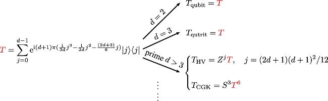
Our T-gates can induce various T-gates in the literature, as illustrated in figure 1.
Figure 1. Various T-gates can be simply derived from our T-gates, which are well defined for arbitrary dimensions. |
5. Constructing MUBs and n-angular frames via T-gates
In this section, we employ the T-gates to construct some special frames including MUBs and certain equidistributed n-angular frames.
Definition 1. Consider a finite normalized frame M = {∣ψα⟩ : α = 1, 2, ⋯ , m}, where ∣ψα⟩ are unit norm vectors in ${{\mathbb{C}}}^{d}$. M is called n-angular if the cardinality of
$\begin{eqnarray*}{\rm{\Lambda }}=\{| \langle {\psi }_{\alpha }| {\psi }_{\beta }\rangle | \,:\alpha \ne \beta \}\end{eqnarray*}$
is exactly n, i.e., Λ = {λj : j = 1, 2, ⋯ , n}. Moreover, M is an equidistributed n-angular frame if $\begin{eqnarray*}\#\{\beta \,:| \langle {\psi }_{\alpha }| {\psi }_{\beta }\rangle | ={\lambda }_{j},\beta =1,2,\cdots \,,\,m\}\end{eqnarray*}$
is a constant independent of α for each j = 1, 2, ⋯ , n.For instance, an equiangular frame is 1-angular and a frame consisting of MUBs is an equidistributed 2-angular frame. A simple approach to equidistributed n-angular frame is through the group frame
$\begin{eqnarray*}{M}_{G,|\psi \rangle }=\{|{\psi }_{\alpha }\rangle ={U}_{\alpha }|\psi \rangle :\alpha =1,2,\cdots \,,\,m\},\end{eqnarray*}$
which is the orbit of a finite group G = {Uα: α = 1, 2, ⋯ , m} (assuming U1 = 1) with a unitary representation on ${{\mathbb{C}}}^{d}$ acting on an initial state ∣ψ⟩. It is known that each group frame constitutes a tight frame on ${{\mathbb{C}}}^{d}$ [64–68]. Moreover, MG,∣ψ⟩ is equidistributed [67, 68], since $\begin{eqnarray*}\langle {\psi }_{\alpha }| {\psi }_{\beta }\rangle =\langle \psi | {U}_{\alpha }^{\dagger }{U}_{\beta }| \psi \rangle =\langle \psi | {\psi }_{\gamma }\rangle ,\end{eqnarray*}$
where ${U}_{\alpha }^{\dagger }{U}_{\beta }={U}_{\gamma }$ is assumed. Consequently, we conclude that {β : ∣⟨ψα∣ψβ⟩∣ = λj, β = 1, 2, ⋯ , m} = {β : ∣⟨ψ∣ψβ⟩∣ = λj, β = 1, 2, ⋯ , m} is independent of α.Consider the group frame generated by ${\mathscr{P}}/U(1)$ (ignoring the global phases) acting on the initial state ∣Uθ⟩ = Uθ∣+⟩, where
$\begin{eqnarray*}{U}_{{\boldsymbol{\theta }}}=\displaystyle \sum _{j=0}^{d-1}{{\rm{e}}}^{{\rm{i}}{\theta }_{j}}| j\rangle \langle j| ,\quad {\theta }_{j}\in [0,2\pi ),\quad | +\rangle =\frac{1}{\sqrt{d}}\displaystyle \sum _{j=0}^{d-1}| j\rangle .\end{eqnarray*}$
Then we obtain an equidistributed frame $\begin{eqnarray*}{M}_{{\mathscr{P}},| {U}_{{\boldsymbol{\theta }}}\rangle }=\{| {U}_{k,l,{\boldsymbol{\theta }}}\rangle ={D}_{k,l}| {U}_{{\boldsymbol{\theta }}}\rangle \,:k,l\in {{\mathbb{Z}}}_{d}\}.\end{eqnarray*}$
Moreover, these d2 unit norm vectors in ${M}_{{\mathscr{P}},| {U}_{{\boldsymbol{\theta }}}\rangle }$ can be divided into d orthonormal bases $\{| {U}_{k,l,{\boldsymbol{\theta }}}\rangle \,:l\in {{\mathbb{Z}}}_{d}\}$ indexed by $k\in {{\mathbb{Z}}}_{d}$, which can be directly verified as $\begin{eqnarray*}\begin{array}{rcl}| \langle {U}_{k,l,{\boldsymbol{\theta }}}| {U}_{k,{l}^{{\prime} },{\boldsymbol{\theta }}}\rangle | & = & | \langle +| {U}_{{\boldsymbol{\theta }}}^{\dagger }{D}_{k,l}^{\dagger }{D}_{k,{l}^{{\prime} }}{U}_{{\boldsymbol{\theta }}}| +\rangle | \\ & = & | \langle +| {U}_{{\boldsymbol{\theta }}}^{\dagger }{Z}^{{l}^{{\prime} }-l}{U}_{{\boldsymbol{\theta }}}| +\rangle | \\ & = & | \langle +| {Z}^{{l}^{{\prime} }-l}| +\rangle | \\ & = & \frac{1}{d}\left|{\sum }_{j=0}^{d-1}{\omega }^{j({l}^{{\prime} }-l)}\right|\\ & = & {\delta }_{l,{l}^{{\prime} }}.\end{array}\end{eqnarray*}$
Specially, when Uθ = 1, we have $\begin{eqnarray*}\{{D}_{k,l}| +\rangle \,:l\in {{\mathbb{Z}}}_{d}\}=\{{Z}^{l}| +\rangle :l\in {{\mathbb{Z}}}_{d}\},\qquad k\in {{\mathbb{Z}}}_{d},\end{eqnarray*}$
which implies that ${M}_{{\mathscr{P}},| +\rangle }$ contains d identical orthonormal bases. When the diagonal gates Uθ = T, we have the following proposition.Proposition 4. For ${{\mathbb{C}}}^{d}$ with computational basis $\{| j\rangle \,:j\in {{\mathbb{Z}}}_{d}\}$, let $| +\rangle =\frac{1}{\sqrt{d}}{\sum }_{j=0}^{d-1}| j\rangle \in {{\mathbb{C}}}^{d}$ be a maximally superposed state and ∣ψ⟩ = T∣+⟩. Let $d={p}_{1}^{{n}_{1}}{p}_{2}^{{n}_{2}}\cdots {p}_{r}^{{n}_{r}}$ be the canonical prime factorization of the dimension d with pi being distinct primes. Consider the following group frame
$\begin{eqnarray}{M}_{{\mathscr{P}},| \psi \rangle }=\{| {\psi }_{k,l}\rangle ={D}_{k,l}| \psi \rangle :k,l\in {{\mathbb{Z}}}_{d}\}.\end{eqnarray}$
We have(1) ${M}_{{\mathscr{P}},| \psi \rangle }$ can be divided into d orthonormal bases $\{| {\psi }_{k,l}\rangle \,:l\in {{\mathbb{Z}}}_{d}\}$ indexed by $k\in {{\mathbb{Z}}}_{d}$.
(2) ${M}_{{\mathscr{P}},| \psi \rangle }$ is an equidistributed n-angular frame, where n = (n1 + 1)(n2 + 1) ⋯ (nr + 1).
Proof. For item (1), this result follows readily from the discussion above.
For item (2) Let
$\begin{eqnarray*}{{\rm{\Lambda }}}_{k,l}=\{|\langle {\psi }_{k,l}|{\psi }_{{k}^{{\rm{{\prime} }}},{l}^{{\rm{{\prime} }}}}\rangle |:{k}^{{\rm{{\prime} }}},{l}^{{\rm{{\prime} }}}\in {{\mathbb{Z}}}_{d}\},\end{eqnarray*}$
then from the properties of group frame we observe that Λk,l = Λ0,0 for any $k,l\in {{\mathbb{Z}}}_{d}$, which imply that ${M}_{{\mathscr{P}},| \psi \rangle }$ is equidistributed. To establish the desired result, it suffices to prove that #Λ0,0 = (n1 + 1)(n2 + 1) ⋯ (nr + 1).Firstly, when k = 0, from the fact that T commutes Z, we have
$\begin{eqnarray*}\begin{array}{rcl}| \langle {\psi }_{0,0}| {\psi }_{0,l}\rangle | & = & | \langle +| {T}^{\dagger }{Z}^{l}T| +\rangle | \\ & = & | \langle +| {Z}^{l}| +\rangle | \\ & = & \frac{1}{d}\left|{\sum }_{j=0}^{d-1}{\omega }^{jl}\right|\\ & = & {\delta }_{0,l}.\end{array}\end{eqnarray*}$
When k > 0, we have $\begin{eqnarray*}\begin{array}{rcl}| \langle {\psi }_{0,0}| {\psi }_{k,l}\rangle | & = & | \langle +| {T}^{\dagger }{X}^{k}{Z}^{l}T| +\rangle | \\ & = & \left|\left\langle +| \left(\displaystyle \sum _{j=0}^{d-1}{{\rm{e}}}^{{\rm{i}}({\theta }_{j}-{\theta }_{j+k})}| j+k\rangle \langle j| \right){Z}^{l}| +\right\rangle \right|\\ & = & \frac{1}{d}\left|\displaystyle \sum _{j=0}^{d-1}{\omega }^{jl}{{\rm{e}}}^{{\rm{i}}({\theta }_{j}-{\theta }_{j+k})}\right|,\end{array}\end{eqnarray*}$
with $\begin{eqnarray*}{\theta }_{j}=\frac{\pi (d+1)}{3d}{j}^{3}-\frac{(d+1)}{2d}{j}^{2}-\frac{(d+1)(2d+3)}{6}j.\end{eqnarray*}$
By direct computation, we obtain that $\begin{eqnarray}\begin{array}{rcl}| \langle {\psi }_{0,0}| {\psi }_{k,l}\rangle | & = & \frac{1}{d}\left|\displaystyle \sum _{j=0}^{d-1}{{\rm{e}}}^{\frac{{\rm{i}}\pi (d+1)}{d}(k{j}^{2}+(k(k-1)-2l)j)}\right|\\ & = & \left\{\begin{array}{l}\frac{1}{d}\left|\displaystyle \sum _{j=0}^{d-1}{\omega }^{k{j}^{2}+(k(k-1)-2l)j}\right|,\quad \omega ={{\rm{e}}}^{{\rm{i}}2\pi /d},\qquad {\rm{for}}\,d\,{\rm{odd}},\\ \frac{1}{2d}\left|\displaystyle \sum _{j=0}^{2d-1}{\tau }^{k{j}^{2}+(k(k-1)-2l)j}\right|,\,\,\tau ={{\rm{e}}}^{{\rm{i}}2\pi /2d},\quad \,\,{\rm{for}}\,d\,{\rm{even}}.\end{array}\right.\end{array}\end{eqnarray}$
We need to consider several cases separately.
(1) k∤d.
When d is odd, from equation (16 ), we have
$\begin{eqnarray*}| \langle {\psi }_{0,0}| {\psi }_{k,l}\rangle | =\frac{1}{d}\left|\displaystyle \sum _{j=0}^{d-1}{\omega }^{k{j}^{2}}\right|=\frac{1}{d}\left|\displaystyle \sum _{j=0}^{d-1}{\omega }^{{j}^{2}}\right|=\frac{1}{\sqrt{d}}.\end{eqnarray*}$
When d is even, k∤d implies k∤2d, and we obtain that
$\begin{eqnarray*}\begin{array}{rcl}| \langle {\psi }_{0,0}| {\psi }_{k,l}\rangle | & = & \frac{1}{2d}\left|\displaystyle \sum _{j=0}^{2d-1}{\tau }^{k{j}^{2}}\right|=\frac{1}{2d}\left|\displaystyle \sum _{j=0}^{2d-1}{\tau }^{{j}^{2}}\right|\\ & = & \frac{| (1+{\rm{i}})\sqrt{2d}| }{2d}=\frac{1}{\sqrt{d}}.\end{array}\end{eqnarray*}$
In summary, we have $| \langle {\psi }_{0,0}| {\psi }_{k,l}\rangle | =1/\sqrt{d}$.
(2) k∣d.
We discuss the cases for odd d and even d separately.
(2.1) When d is odd, let m = gcd(d, k) > 1. We consider the following two cases m∤(k(k − 1) − 2l) and m∣(k(k − 1) − 2l). When l runs through {0, 1, ⋯ , d − 1}, the value of (k(k − 1) − 2l) can take any value in {0, 1, ⋯ , d − 1}.
(2.1a) m∤(k(k − 1) − 2l)
In this case, we have the quadratic Gauss sum ${\sum }_{j=0}^{d-1}{\omega }^{k{j}^{2}+(k(k-1)-2l)j}=0$. Consequently, we obtain that ∣⟨ψ0,0∣ψk,l⟩∣ = 0.
(2.1b) m∣(k(k − 1) − 2l)
Let ${d}^{{\prime} }=d/m,{k}^{{\prime} }=k/m,{r}^{{\prime} }=(k(k-1)-2l)/m$ be integers and let $\gamma ={{\rm{e}}}^{{\rm{i}}2\pi /{d}^{{\prime} }}$. In this case, we have the quadratic Gauss sum
$\begin{eqnarray*}\begin{array}{l}\left|\displaystyle \sum _{j=0}^{d-1}{\omega }^{k{j}^{2}+(k(k-1)-2l)j}\right|=m\left|\displaystyle \sum _{j=0}^{d^{\prime} -1}{\gamma }^{k^{\prime} {j}^{2}+r^{\prime} j}\right|\\ =m\left|\displaystyle \sum _{j=0}^{d^{\prime} -1}{\gamma }^{k^{\prime} {j}^{2}}\right|=m\left|\displaystyle \sum _{j=0}^{d^{\prime} -1}{\gamma }^{{j}^{2}}\right|=m\sqrt{d^{\prime} },\end{array}\end{eqnarray*}$
since ${d}^{{\prime} }$ is also an odd number. Consequently, we have $\begin{eqnarray*}| \langle {\psi }_{0,0}| {\psi }_{k,l}\rangle | =\frac{1}{d}\left|\displaystyle \sum _{j=0}^{d-1}{\omega }^{k{j}^{2}+(k(k-1)-2l)j}\right|=\frac{m\sqrt{{d}^{{\prime} }}}{d}=\frac{1}{\sqrt{{d}^{{\prime} }}}.\end{eqnarray*}$
Here, ${d}^{{\prime} }| d$ and ${d}^{{\prime} }\lt d$.(2.2) When d is even, let m = gcd(d, k) > 1. We consider the following two cases gcd(2d, k)∤(k(k − 1) − 2l) and gcd(2d, k)∣(k(k − 1) − 2l). When l runs through {0, 1, ⋯ , d − 1}, the value of (k(k − 1) − 2l)/2 can take any value in {0, 1, ⋯ , d − 1}.
(2.2a) gcd(2d, k)∤(k(k − 1) − 2l).
In this case, the quadratic Gauss sum ${\sum }_{j=0}^{d-1}{\tau }^{(k{j}^{2}+(k(k-1)-2l)j)}=0$. Consequently, we obtain that ∣⟨ψ0,0∣ψk,l⟩∣ = 0.
(2.2b) gcd(2d, k)∣(k(k − 1) − 2l).
Let ${d}^{{\prime} }=d/m$.
If ${d}^{{\prime} }$ is even, then m = gcd(d, k) = gcd(2d, k) > 1. Let ${k}^{{\prime} }=k/m,{r}^{{\prime} }=(k(k-1)-2l)/m$ be integers and let $\zeta ={{\rm{e}}}^{{\rm{i}}2\pi /2{d}^{{\prime} }}={{\rm{e}}}^{{\rm{i}}\pi /{d}^{{\prime} }}$. In this case, we have the quadratic Gauss sum
$\begin{eqnarray*}\begin{array}{l}\left|\displaystyle \sum _{j=0}^{2d-1}{\tau }^{k{j}^{2}+(k(k-1)-2l)j}\right|=m\left|\displaystyle \sum _{j=0}^{2d^{\prime} -1}{\zeta }^{k^{\prime} {j}^{2}+r^{\prime} j}\right|\\ =m\left|\displaystyle \sum _{j=0}^{2d^{\prime} -1}{\zeta }^{k^{\prime} {j}^{2}}\right|=m\left|\displaystyle \sum _{j=0}^{2d^{\prime} -1}{\zeta }^{{j}^{2}}\right|\\ =m| (1+{\rm{i}})\sqrt{2{d}^{{\prime} }}| =2m\sqrt{{d}^{{\prime} }}.\end{array}\end{eqnarray*}$
Consequently, we obtain $\begin{eqnarray*}\begin{array}{rcl}| \langle {\psi }_{0,0}| {\psi }_{k,l}\rangle | & = & \frac{1}{2d}\left|\displaystyle \sum _{j=0}^{2d-1}{\tau }^{k{j}^{2}+(k(k-1)-2l)j}\right|\\ & = & \frac{2m\sqrt{{d}^{{\prime} }}}{2d}=\frac{1}{\sqrt{{d}^{{\prime} }}}.\end{array}\end{eqnarray*}$
If ${d}^{{\prime} }$ is odd, then gcd(2d, k) = 2gcd(d, k) = 2m. Let ${k}^{{\prime} }=k/2\,m,{r}^{{\prime} }=(k(k-1)-2l)/2m$ be integers and let $\gamma ={{\rm{e}}}^{{\rm{i}}2\pi /{d}^{{\prime} }}$. In this case, we have the quadratic Gauss sum
$\begin{eqnarray*}\begin{array}{l}\left|\displaystyle \sum _{j=0}^{2d-1}{\tau }^{k{j}^{2}+(k(k-1)-2l)j}\right|=2m\left|\displaystyle \sum _{j=0}^{{d}^{{\prime} }-1}{\gamma }^{k^{\prime} {j}^{2}+r^{\prime} j}\right|\\ =2m\left|\displaystyle \sum _{j=0}^{{d}^{{\prime} }-1}{\gamma }^{k^{\prime} {j}^{2}}\right|=2m\left|\displaystyle \sum _{j=0}^{{d}^{{\prime} }-1}{\gamma }^{{j}^{2}}\right|=2m\sqrt{{d}^{{\prime} }}.\end{array}\end{eqnarray*}$
Consequently, we obtain $\begin{eqnarray*}\begin{array}{rcl}| \langle {\psi }_{0,0}| {\psi }_{k,l}\rangle | & = & \frac{1}{2d}\left|\displaystyle \sum _{j=0}^{2d-1}{\tau }^{k{j}^{2}+(k(k-1)-2l)j}\right|\\ & = & \frac{2m\sqrt{{d}^{{\prime} }}}{2d}=\frac{1}{\sqrt{{d}^{{\prime} }}}.\end{array}\end{eqnarray*}$
In summary, we have $| \langle {\psi }_{0,0}| {\psi }_{k,l}\rangle | =1/\sqrt{{d}^{{\prime} }}$, where ${d}^{{\prime} }| d$ and ${d}^{{\prime} }\lt d$.Combining the two cases k∣d and k∤d, we obtain that
$\begin{eqnarray*}{{\rm{\Lambda }}}_{0,0}=\left\{\frac{1}{\sqrt{{d}^{{\prime} }}}:{d}^{{\prime} }| d,{d}^{{\prime} }\ne 1\right\}\cup \{0\}.\end{eqnarray*}$
Finally, we have the cardinality $\begin{eqnarray*}| {{\rm{\Lambda }}}_{0,0}| =({n}_{1}+1)({n}_{2}+1)\cdots ({n}_{r}+1),\end{eqnarray*}$
since $d={p}_{1}^{{n}_{1}}{p}_{2}^{{n}_{2}}\cdots {p}_{r}^{{n}_{r}}$ with pi being distinct primes.It is remarkable that when d is a prime number, the group frame defined by equation (15 ) can actually be partitioned into d MUBs, since ${{\rm{\Lambda }}}_{0,0}=\{1/\sqrt{{d}^{{\prime} }}:{d}^{{\prime} }| d,{d}^{{\prime} }\ne 1\}\cup \{0\}\,=\{0,1/\sqrt{d}\}$. These d MUBs, together with the computational basis $\{| j\rangle \,:j\in {{\mathbb{Z}}}_{d}\}$ of ${{\mathbb{C}}}^{d}$, constitute a complete family of d + 1 MUBs of ${{\mathbb{C}}}^{d}$.
6. Discussion
According to the Gottesman–Knill theorem, non-Clifford gates, in particular, the T-gates, are essential for achieving universal quantum computation. Considering the significance of T-gates in discrete-variable quantum computation, it is desirable to study such gates in arbitrary finite dimensional systems. However, in the literature, the T-gates are only defined in prime dimensional systems, and their non-prime dimensional analogies remain elusive. In this work, inspired by the cubic phase gates in continuous-variable systems and the analogies between the Clifford/non-Clifford gates in discrete-variable systems and the Gaussian/non-Gaussian gates in continuous-variable systems, we have introduced general T-gates in arbitrary finite dimensional systems via GKP encoding.
As a bridge between discrete- and continuous-variable systems, GKP encoding maps quantum states in discrete-variable systems to (generalized) quantum states in continuous-variable systems, and can be used to connect discrete-variable gates and continuous-variable ones. We have exploited an important class of non-Gaussian gates, i.e., the class of cubic phase gates, in order to derive discrete-variable T-gates. This is achieved by determining the parameters in the cubic phase gates preserving the GKP code space. We are then led, via GKP encoding, to T-gates in arbitrary dimensional systems, circumventing number-theoretic challenges in the conventional approach to T-gates. We have compared our T-gates with those in the literature, and have shown that they indeed generalize the existing ones. We have introduced the Gaussian hierarchy as a continuous-variable analogy of the discrete-variable Clifford hierarchy. As an interesting application of our T-gates, we have provided a simple method for constructing MUBs and n-angular frames.
Our GKP-induced T-gates are defined in arbitrary finite dimensional systems, enabling the extension of the ‘Clifford+T’framework to any finite dimensional system. Many features and implications of the T-gates remain to be investigated. We hope the T-gates can be used to study the Clifford hierarchy, in particular the group structures of diagonal gates. It is also reasonable to expect that the T-gates are optimal in generating magic (non-stabilizer) resources in some sense [26–28]. Furthermore, exploring the role of T-gates in fault-tolerant quantum computation, particularly in magic state distillation [69], may reveal practical advantage in non-prime dimensions. It would also be valuable to examine the feasibility of T-gate teleportation in general dimensions. The relationship between even higher order continuous-variable phase gates and Clifford hierarchy gates in both single- and multi-qudit gates remains an intriguing issue for future research. It is known that certain bizarre physical phenomena occur in non-prime dimensions, in contrast to prime dimensions, and it is expected that GKP encoding can provide insights into such phenomena. Finally, while it is natural to use GKP encoding to establish the discrete- and continuous-variable bridge, it is also desirable to investigate some axiomatic reasoning from which GKP encoding or other alternative encodings emerge. These issues will be treated elsewhere. In summary, the interplay between discrete- and continuous-variable systems via GKP encoding is worth further investigations for both its own intrinsic significance and practical applications.