


1. Introduction
The Standard Model (SM) of particle physics represents our best understanding of nature, as it explains three of the four fundamental forces that govern the universe. Up to now, the SM has successfully explained almost all observations from collider experiments; while it fails to explain some fundamental problems, like neutrino masses and the dark matter, which suggests new physics beyond the Standard Model. With the advent of experimental techniques, particularly the upgrades of the Large Hadron Collider (LHC) [1, 2], and the upcoming new colliders [3–10], high-energy scattering processes will be explored attentively and precisely. Meanwhile, searching for new physics requires that the established theory provides sufficiently accurate predictions for the observations. For this sake, pursuing a higher order calculation of perturbation theory is clearly a major task of physicists.
A fundamental technical difficulty in higher order calculation is the treatment of Feynman integrals. Over past decades, a variety of representations for Feynman integrals have been developed, including the Schwinger parameters representation [11], the Feynman parameters representation [12], the Mellin–Barnes representation [13, 14], the Lee–Pomeransky representation [15], and the Baikov representation [16]. Another effective approach for evaluating multi-loop integrals is the differential equations method, which has attracted wide interest in the academic community [17–22]. Some notable progress in recent years includes the uniform transcendental (UT) basis method proposed in [23], which can simplify the differential equations significantly; and the auxiliary mass flow method proposed in [24, 25], which can provide high-precision numerical results efficiently.
In this paper, we study three classes of Feynman integrals: the massless banana integral, the one-mass banana integral, and the massless three-point multi-edge integral. We find that the any loop analytic results of these integrals can be obtained by recursively using the one-loop integration formulas, and the results turn out to be quite simple and compact. The computational details and results for each integral are subsequently presented in sections 2 –4 . The application of this method in a more general case is discussed in section 5 . In the last section, we present discussions and a conclusion.
2. Massless banana integral
In this section we consider the massless L-loop banana graph, which is shown in figure 1(a), wherein the external momentum is denoted by q, the loop momenta are denoted by ki (i = 1, …, L). The spacetime dimensions are set to be d = 4 − 2ε. The Feynman integral of this graph is defined as 3 ) twice6 ) by using the mathematical induction method. Considering the (L + 1)-loop integral shown in figure 1(b), the L-loop substructure can be constructed by using equation (6 ), we then obtain 6 ).
$\begin{eqnarray}{I}_{1}^{(L)}(q,\{{a}_{i}\})=\int \left(\displaystyle \prod _{i=1}^{L}\frac{{\,\rm{d}\,}^{d}{k}_{i}}{i{\pi }^{d/2}}\right)\left(\displaystyle \prod _{j=1}^{L+1}\frac{1}{{D}_{j}^{{a}_{j}}}\right),\end{eqnarray}$
with the inverse of propagators parametrized as $\begin{eqnarray}\begin{array}{rcl}{D}_{1} & = & -{k}_{1}^{2},\quad {D}_{2}=-{({k}_{2}-{k}_{1})}^{2},\,\cdots \,,\\ {D}_{L} & = & -{({k}_{L}-{k}_{L-1})}^{2},\\ {D}_{L+1} & = & -{(q-{k}_{L})}^{2}.\end{array}\end{eqnarray}$
We start from the L = 1 case, for which the one-loop integral can be calculated directly by using the Feynman parameters representation [13] $\begin{eqnarray}\begin{array}{rcl}{I}_{1}^{(1)}\left(q,\{{a}_{1},{a}_{2}\}\right) & = & \displaystyle \int \frac{{\,\rm{d}\,}^{d}{k}_{1}}{i{\pi }^{d/2}}\frac{1}{{[-{k}_{1}^{2}]}^{{a}_{1}}{[-{(q-{k}_{1})}^{2}]}^{{a}_{2}}}\\ & = & \frac{G({a}_{1},{a}_{2})}{{(-{q}^{2})}^{{a}_{1}+{a}_{2}-d/2}},\end{array}\end{eqnarray}$
where $\begin{eqnarray}G({a}_{1},{a}_{2})=\frac{{\rm{\Gamma }}\left({a}_{1}+{a}_{2}-\frac{d}{2}\right){\rm{\Gamma }}\left(\frac{d}{2}-{a}_{1}\right){\rm{\Gamma }}\left(\frac{d}{2}-{a}_{2}\right)}{{\rm{\Gamma }}({a}_{1}){\rm{\Gamma }}({a}_{2}){\rm{\Gamma }}(d-{a}_{1}-{a}_{2})}.\end{eqnarray}$
Then the two-loop sunrise integral can be evaluated by using equation ( $\begin{eqnarray}\begin{array}{rcl}{I}_{1}^{(2)}\left(q,\{{a}_{1},{a}_{2},{a}_{3}\}\right) & = & \displaystyle \int \frac{{\rm{d}\,}^{d}{k}_{1}}{i{\pi }^{d/2}}\frac{{\,\rm{d}}^{d}{k}_{2}}{i{\pi }^{d/2}}\frac{1}{{[-{k}_{1}^{2}]}^{{a}_{1}}{[-{({k}_{2}-{k}_{1})}^{2}]}^{{a}_{2}}{[-{(q-{k}_{2})}^{2}]}^{{a}_{3}}}\\ & = & G({a}_{1},{a}_{2})\displaystyle \int \frac{{\,\rm{d}\,}^{d}{k}_{2}}{i{\pi }^{d/2}}\frac{1}{{[-{k}_{2}^{2}]}^{{a}_{1}+{a}_{2}-d/2}{[-{(q-{k}_{2})}^{2}]}^{{a}_{3}}}\\ & = & \frac{G({a}_{1},{a}_{2})G\left({a}_{1}+{a}_{2}-\frac{d}{2},{a}_{3}\right)}{{(-{q}^{2})}^{{a}_{1}+{a}_{2}+{a}_{3}-d}}.\end{array}\end{eqnarray}$
By repeating this procedure L times, we obtain the result at L-loop order $\begin{eqnarray}\begin{array}{rcl}{I}_{1}^{(L)}\left(q,\{{a}_{i}\}\right) & = & \frac{1}{{(-{q}^{2})}^{{A}_{L+1}}}\displaystyle \prod _{i=1}^{L}G({A}_{i},{a}_{i+1})\\ & = & \frac{1}{{(-{q}^{2})}^{{A}_{L+1}}}\frac{{\rm{\Gamma }}({A}_{L+1})}{{\rm{\Gamma }}\left(\frac{d}{2}-{A}_{L+1}\right)}\displaystyle \prod _{i=1}^{L+1}\frac{{\rm{\Gamma }}\left(\frac{d}{2}-{a}_{i}\right)}{{\rm{\Gamma }}({a}_{i})}.\end{array}\end{eqnarray}$
Here, for brevity, we introduce the notation ${A}_{n}\,={\sum }_{i=1}^{n}\left({a}_{i}-\frac{d}{2}\right)+\frac{d}{2}$. We may complete the proof of equation ( $\begin{eqnarray}\begin{array}{rcl}{I}_{1}^{(L+1)}\left(q,\{{a}_{i}\}\right) & = & \displaystyle \int \frac{{\,\rm{d}\,}^{d}{k}_{L+1}}{i{\pi }^{d/2}}\,{I}_{1}^{(L)}({k}_{L+1},\{{a}_{i}\})\\ & & \times \frac{1}{{[-(q-{k}_{L+1})]}^{{a}_{L+2}}}\\ & = & \displaystyle \prod _{i=1}^{L}G({A}_{i},{a}_{i+1})\displaystyle \int \frac{{\,\rm{d}\,}^{d}{k}_{L+1}}{i{\pi }^{d/2}}\,\\ & & \times \frac{1}{{(-{k}_{L+1}^{2})}^{{A}_{L+1}}}\frac{1}{{[-(q-{k}_{L+1})]}^{{a}_{L+2}}}\\ & = & \frac{1}{{(-{q}^{2})}^{{A}_{L+2}}}\displaystyle \prod _{i=1}^{L+1}G({A}_{i},{a}_{i+1}),\end{array}\end{eqnarray}$
which is in the same form as equation (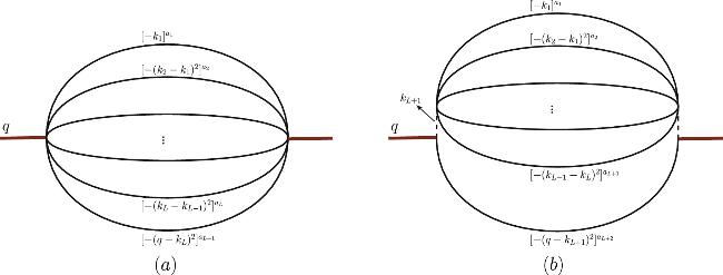
Figure 1. (a) The massless L-loop banana graph. (b) The massless (L + 1)-loop banana graph. |
The UT basis ensures that each term in the expansion of ε possesses the same transcendentality. We then try to find out the UT basis for the L-loop banana ${I}_{1}^{(L)}(q,\{{a}_{i}\})$. It is known that the one-loop integral $\int {\,\rm{d}\,}^{d}k{[-{k}^{2}]}^{-1}{[-{(q-k)}^{2}]}^{-2}$ possesses the uniform transcendentality. On the other hand, according to the second line of equation (7 ), the ratio between ${I}_{1}^{(L)}$ and ${I}_{1}^{(L-1)}$ is ${I}_{1}^{(L)}/{I}_{1}^{(L-1)}\sim \int {\,\rm{d}\,}^{d}{k}_{L}{[-{k}_{L}^{2}]}^{-{A}_{L}}{[-{(q-{k}_{L})}^{2}]}^{-{a}_{L+1}}$. Hence, the UT basis can be obtained by demanding ${A}_{L}\sim 1+{ \mathcal O }(\epsilon )$ and aL+1 = 2, which eventually leads to a1 = 1, a2 = ⋯ = aL+1 = 2. Therefore, the UT basis takes the form 8 ) up to a five-loop order
$\begin{eqnarray}\begin{array}{rcl}{I}_{1}^{(L)}\left(q,\{1,\mathop{\underbrace{2,\ldots ,2}}\limits_{L}\}\right) & = & \frac{1}{{(-{q}^{2})}^{1+L\epsilon }}\\ & & \times \frac{{\rm{\Gamma }}\left(1+L\epsilon \right){\rm{\Gamma }}(1-\epsilon ){\rm{\Gamma }}{(-\epsilon )}^{L}}{{\rm{\Gamma }}\left(1-(L+1)\epsilon \right)},\end{array}\end{eqnarray}$
which is remarkably simple. As an illustration, we present the ε-expansion series of equation ( $\begin{eqnarray}{\tilde{I}}_{1}^{(1)}=-\frac{1}{\epsilon }+\frac{{\pi }^{2}}{12}\epsilon +\frac{7\zeta (3)}{3}{\epsilon }^{2}+O({\epsilon }^{3}).\end{eqnarray}$
$\begin{eqnarray}{\tilde{I}}_{1}^{(2)}=\frac{1}{{\epsilon }^{2}}-\frac{{\pi }^{2}}{6}-\frac{32\zeta (3)\epsilon }{3}-\frac{19{\pi }^{4}{\epsilon }^{2}}{120}+O({\epsilon }^{3}).\end{eqnarray}$
$\begin{eqnarray}\begin{array}{rcl}{\tilde{I}}_{1}^{(3)} & = & -\frac{1}{{\epsilon }^{3}}+\frac{{\pi }^{2}}{4\epsilon }+29\zeta (3)+\frac{71{\pi }^{4}\epsilon }{160}\\ & & +\,\left[\frac{1263\zeta (5)}{5}-\frac{29{\pi }^{2}\zeta (3)}{4}\right]{\epsilon }^{2}+O({\epsilon }^{3}).\end{array}\end{eqnarray}$
$\begin{eqnarray}\begin{array}{rcl}{\tilde{I}}_{1}^{(4)} & = & \frac{1}{{\epsilon }^{4}}-\frac{{\pi }^{2}}{3{\epsilon }^{2}}-\frac{184\zeta (3)}{3\epsilon }-\frac{43{\pi }^{4}}{45}\\ & & +\left[\frac{184{\pi }^{2}\zeta (3)}{9}-\frac{4144\zeta (5)}{5}\right]\epsilon \\ & & +\left[\frac{16928\zeta {(3)}^{2}}{9}-\frac{536{\pi }^{6}}{315}\right]{\epsilon }^{2}+O({\epsilon }^{3}).\end{array}\end{eqnarray}$
$\begin{eqnarray}\begin{array}{rcl}{\tilde{I}}_{1}^{(5)} & = & -\frac{1}{{\epsilon }^{5}}+\frac{5{\pi }^{2}}{12{\epsilon }^{3}}+\frac{335\zeta (3)}{3{\epsilon }^{2}}+\frac{169{\pi }^{4}}{96\epsilon }+2179\zeta (5)\\ & & -\,\frac{1675{\pi }^{2}\zeta (3)}{36}+\left[\frac{38015{\pi }^{6}}{8064}-\frac{112225\zeta {(3)}^{2}}{18}\right]\epsilon \\ & & +\,\left[\frac{358055\zeta (7)}{7}-\frac{56615{\pi }^{4}\zeta (3)}{288}-\frac{10895{\pi }^{2}\zeta (5)}{12}\right]{\epsilon }^{2}+O({\epsilon }^{3}).\end{array}\end{eqnarray}$
Here, for for brevity, we introduce the notation${\tilde{I}}_{1}^{(L)}={\rm{e}\,}^{L{\gamma }_{\,\rm{E}}\epsilon }{(-{q}^{2})}^{1+L\epsilon }{I}_{1}^{(L)}(q,\{1,2,\ldots ,2\})$.Note that in d = 2 − 2ε, the UT basis has a more concise form, with ${I}_{1}^{(L)}\left(q,\{1,\mathop{\underbrace{1,\ldots ,1}}\limits_{L}\}\right)$ naturally forming the UT basis, and we can use the dimension shift to recover the UT basis in d = 4 − 2ε.
3. One-mass banana integral
In this section and the following ones, we investigate the case where the massless banana appears as a subgraph of a bigger graph. Equation (6 ) indicates that the integration of a banana subgraph will not lead to too much complexity, but only a shift on the power of the propagator. In this way, the multi-loop integral is reduced to the one-loop integral with non-integer propagator power.
We first consider the banana integral with one massive propagator. One may encounter this integral when calculating the total decay width of a heavy quark [26, 27]. The corresponding graph is shown in figure 2(a). Denoting the external momentum as q, the loop momenta as ki (i = 1, …, L), the general expression of this integral is 14 ) can be carried out by using equation (6 ). Therefore, we have 6 ), the L-loop integral reduces to a one-loop integral, as shown in figure 2(b). On the other hand, the two-point one-loop integral with arbitrary propagator powers has been investigated in [28–31]. By using their results, we finally obtain
$\begin{eqnarray}{I}_{2}^{(L)}\left(q,\{{a}_{i}\},{b}_{1}\right)=\int \left(\displaystyle \prod _{i=1}^{L}\frac{{\,\rm{d}\,}^{d}{k}_{i}}{i{\pi }^{d/2}}\right)\left(\displaystyle \prod _{j=1}^{L}\frac{1}{{D}_{1,j}^{{a}_{j}}}\right)\frac{1}{{D}_{2}^{{b}_{1}}},\end{eqnarray}$
where the inverse of the propagators read $\begin{eqnarray}\begin{array}{l}{D}_{1,1}=-{k}_{1}^{2},\quad {D}_{1,2}=-{({k}_{2}-{k}_{1})}^{2},\,\cdots \,,\\ {D}_{1,L}=-{({k}_{L}-{k}_{L-1})}^{2},\\ {D}_{2}={m}^{2}-{(q-{k}_{L})}^{2}.\end{array}\end{eqnarray}$
The intermediate integrations over k1 to kL−1 of equation ( $\begin{eqnarray}\begin{array}{rcl}{I}_{2}^{(L)}\left(q,\{{a}_{i}\},{b}_{1}\right) & = & \frac{{\rm{\Gamma }}({A}_{L})}{{\rm{\Gamma }}\left(\frac{d}{2}-{A}_{L}\right)}\displaystyle \prod _{i=1}^{L}\frac{{\rm{\Gamma }}\left(\frac{d}{2}-{a}_{i}\right)}{{\rm{\Gamma }}({a}_{i})}\\ & & \times \,\displaystyle \int \frac{{\,\rm{d}\,}^{d}{k}_{L}}{i{\pi }^{d/2}}\frac{1}{{[-{k}_{L}^{2}]}^{{A}_{L}}{[{m}^{2}-{(q-{k}_{L})}^{2}]}^{{b}_{1}}},\end{array}\end{eqnarray}$
which indicates that after using equation ( $\begin{eqnarray}\begin{array}{rcl}{I}_{2}^{(L)}\left(q,\{{a}_{i}\},{b}_{1}\right) & = & \frac{1}{{({m}^{2})}^{{A}_{L}+{b}_{1}-d/2}}\\ & & \times \frac{{\rm{\Gamma }}\left({A}_{L}\right){\rm{\Gamma }}\left({A}_{L}+{b}_{1}-\frac{d}{2}\right)}{{\rm{\Gamma }}\left(\frac{d}{2}\right){\rm{\Gamma }}({b}_{1})}\displaystyle \prod _{i=1}^{L}\frac{{\rm{\Gamma }}\left(\frac{d}{2}-{a}_{i}\right)}{{\rm{\Gamma }}({a}_{i})}\\ & & \times {\,}_{2}{F}_{1}\left({A}_{L},{A}_{L}+{b}_{1}-\frac{d}{2};\frac{d}{2};\frac{{q}^{2}}{{m}^{2}}\right).\end{array}\end{eqnarray}$
Here, 2F1 is the hypergeometric function. For the special cases where the external momentum goes on-shell or vanishes, we have $\begin{eqnarray}\begin{array}{rcl}{I}_{2}^{(L)}\left(q,\{{a}_{i}\},{b}_{1}\right) & \mathop{\to }\limits^{{q}^{2}\to {m}^{2}} & \frac{1}{{({m}^{2})}^{{A}_{L}+{b}_{1}-d/2}}\\ & & \quad \times \,\frac{{\rm{\Gamma }}\left({A}_{L}\right){\rm{\Gamma }}\left({A}_{L}+{b}_{1}-\frac{d}{2}\right){\rm{\Gamma }}\left(d-2{A}_{L}-{b}_{1}\right)}{{\rm{\Gamma }}\left(\frac{d}{2}-{A}_{L}\right){\rm{\Gamma }}\left(d-{A}_{L}-{b}_{1}\right){\rm{\Gamma }}({b}_{1})}\\ & & \quad \times \,\displaystyle \prod _{i=1}^{L}\frac{{\rm{\Gamma }}\left(\frac{d}{2}-{a}_{i}\right)}{{\rm{\Gamma }}({a}_{i})},\end{array}\end{eqnarray}$
$\begin{eqnarray}\begin{array}{rcl}{I}_{2}^{(L)}\left(q,\{{a}_{i}\},{b}_{1}\right) & \mathop{\to }\limits^{{q}^{2}\to 0} & \frac{1}{{({m}^{2})}^{{A}_{L}+{b}_{1}-d/2}}\frac{{\rm{\Gamma }}\left({A}_{L}\right){\rm{\Gamma }}\left({A}_{L}+{b}_{1}-\frac{d}{2}\right)}{{\rm{\Gamma }}\left(\frac{d}{2}\right){\rm{\Gamma }}({b}_{1})}\\ & & \times \,\displaystyle \prod _{i=1}^{L}\frac{{\rm{\Gamma }}\left(\frac{d}{2}-{a}_{i}\right)}{{\rm{\Gamma }}({a}_{i})}.\end{array}\end{eqnarray}$
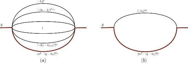
Figure 2. (a) The one-mass L-loop banana graph. (b) The reduced graph after using equation ( |
Like the case of the massless banana integral, one of the UT basis can be constructed by setting a1 = 1, a2 = ⋯ = aL = 2, b1 = 2, that is
$\begin{eqnarray}\begin{array}{rcl}{I}_{2}^{(L)}\left(q,\{1,\mathop{\underbrace{2,\ldots ,2}}\limits_{L-1}\},2\right) & = & \frac{{\rm{\Gamma }}(1-\epsilon ){\rm{\Gamma }}{(-\epsilon )}^{L-1}}{{({m}^{2})}^{1+L\epsilon }}\frac{{\rm{\Gamma }}\left(1+(L-1)\epsilon \right){\rm{\Gamma }}\left(1+L\epsilon \right)}{{\rm{\Gamma }}\left(\frac{d}{2}\right)}\\ & & {\times \,}_{2}{F}_{1}\left(1+(L-1)\epsilon ,1+L\epsilon ;2-\epsilon ;\frac{{q}^{2}}{{m}^{2}}\right),\end{array}\end{eqnarray}$
which can be expanded with the help of HypExp [32]: $\begin{eqnarray}x{\tilde{I}}_{2}^{(1)}=-{\mathrm{ln}}\,(1-x)+O(\epsilon ),\end{eqnarray}$
$\begin{eqnarray}x{\tilde{I}}_{2}^{(2)}=\frac{{\mathrm{ln}}\,(1-x)}{\epsilon }-{\,\rm{Li}\,}_{2}(x)-2\,{{\mathrm{ln}}}^{2}(1-x)+O(\epsilon ),\end{eqnarray}$
$\begin{eqnarray}\begin{array}{rcl}x{\tilde{I}}_{2}^{(3)} & = & -\frac{{\mathrm{ln}}\,(1-x)}{{\epsilon }^{2}}+\left[{\,\rm{Li}\,}_{2}(x)+3\,{{\mathrm{ln}}}^{2}(1-x)\right]\frac{1}{\epsilon }\\ & & +18{\,\rm{Li}\,}_{3}(1-x)+{\,\rm{Li}\,}_{3}(x)+6{\,\rm{Li}\,}_{2}(x)\,{\mathrm{ln}}\,(1-x)\\ & & -\,6\,{{\mathrm{ln}}}^{3}\,(1-x)+9\,{{\mathrm{ln}}}^{2}\,(1-x)\,{\mathrm{ln}}\,x\\ & & -\frac{17}{4}{\pi }^{2}\,{\mathrm{ln}}\,(1-x)-18\zeta (3)+O(\epsilon ),\end{array}\end{eqnarray}$
$\begin{eqnarray}\begin{array}{rcl}x{\tilde{I}}_{2}^{(4)} & = & \frac{{\mathrm{ln}}\,(1-x)}{{\epsilon }^{3}}-\left[{\,\rm{Li}\,}_{2}(x)+4\,{{\mathrm{ln}}}^{2}\,(1-x)\right]\frac{1}{{\epsilon }^{2}}\\ & & +\left[-96{\,\rm{Li}\,}_{3}(1-x)-3{\,\rm{Li}\,}_{3}(x)\right.\\ & & -\,36{\,\rm{Li}\,}_{2}(x)\,{\mathrm{ln}}\,(1-x)+32\,{{\mathrm{ln}}}^{3}\,(1-x)\\ & & -48\,{\mathrm{ln}}\,x\,{{\mathrm{ln}}}^{2}\,(1-x)+23{\pi }^{2}\,{\mathrm{ln}}\,(1-x)\\ & & \left.+\,96\zeta (3)\right]\frac{1}{3\epsilon }+32{\,\rm{Li}\,}_{4}\left(\frac{x}{x-1}\right)+32{\,\rm{Li}\,}_{4}(1-x)\\ & & +31{\,\rm{Li}\,}_{4}(x)-12{\,\rm{Li}\,}_{3}(x)\,{\mathrm{ln}}\,(1-x)\\ & & +\,96{\,\rm{Li}\,}_{3}(1-x)\,{\mathrm{ln}}\,(1-x)+{\,\rm{Li}\,}_{2}(x)\\ & & \times \,\left(48\,{{\mathrm{ln}}}^{2}\,(1-x)-\frac{7}{3}{\pi }^{2}\right)-\frac{472}{3}\zeta (3)\,{\mathrm{ln}}\,(1-x)\\ & & -\,20\,{{\mathrm{ln}}}^{4}\,(1-x)+\frac{160}{3}\,{{\mathrm{ln}}}^{3}\,(1-x)\,{\mathrm{ln}}\,x\\ & & -28{\pi }^{2}\,{{\mathrm{ln}}}^{2}\,(1-x)-\frac{16}{45}{\pi }^{4}+O(\epsilon ).\end{array}\end{eqnarray}$
Here, for for brevity, we introduce the notation ${\tilde{I}}_{2}^{(L)}\,={\rm{e}\,}^{L{\gamma }_{\,\rm{E}}\epsilon }{(-{q}^{2})}^{1+L\epsilon }{I}_{2}^{(L)}(q,\{1,2,\ldots ,2\},2)$, and x = q2/m2.Beyond the one-loop order, we find that the integral family considered in this sector contains two master integrals. We inductively construct the UT basis at any loop order, they are 19 ). The analytic results for these integrals can alternatively be derived through an iterative procedure of solving the canonical differential equations order by order within the framework of ε-expansion.
$\begin{eqnarray}\begin{array}{rcl}{\boldsymbol{F}} & = & \{({q}^{2}-{m}^{2}){I}_{2}^{(L)}\left(q,\{\mathop{\underbrace{2,\ldots ,2}}\limits_{L}\},1\right)-L\,{m}^{2}\,{I}_{2}^{(L)}\left(q,\{1,\mathop{\underbrace{2,\ldots ,2}}\limits_{L-1}\},2\right),\\ & & {q}^{2}{I}_{2}^{(L)}\left(q,\{1,\mathop{\underbrace{2,\ldots ,2}}\limits_{L-1}\},2\right)\},\end{array}\end{eqnarray}$
with the corresponding differential equations formulated as $\begin{eqnarray}\frac{{\rm{d}}\,{\boldsymbol{F}}}{{\rm{d}}x}=\epsilon \left[\begin{array}{cc}-\frac{L}{x-1} & {L}^{2}\left(\frac{1}{x}-\frac{1}{x-1}\right)\\ -\frac{1}{x-1} & \frac{1}{x}-\frac{L}{x-1}\\ \end{array}\right]\cdot {\boldsymbol{F}},\end{eqnarray}$
where L is the number of loop. The above differential equations are in canonical form, and there are two letters that appeared in the alphabet {x, 1 − x}. The integrals are regular at q2 = 0, the boundary conditions for the basis at q2 = 0 can readily be obtained from equation (4. Massless three-point multi-edge integral
In this section, we consider the massless three-point multi-edge integral. This integral is involved in the calculation of the massless form factor [33, 34]. The corresponding graph is shown in figure 3(a), wherein, the external momenta is denoted by q, q1, q2, with overall momentum conservation q = q1 + q2; the loop momenta are denoted by k0, k1,i, k2,i, and k3,i; the number of edges at each side is denoted by m, n, l, respectively, and hence the loop number is L = m + n + l − 2. We consider the special case where ${q}_{1}^{2}={q}_{2}^{2}=0$. The general expression of this integral is 6 ), we have 31 ) is shown in figure 3(b). In combination with the studies of [28, 30], we obtain the final result
$\begin{eqnarray}\begin{array}{rcl} & & {I}_{3}^{(m+n+l-2)}\left(q,\{{a}_{i}\},\{{b}_{i}\},\{{c}_{i}\}\right)\\ & & \quad =\displaystyle \int \frac{{\,\rm{d}\,}^{d}{k}_{0}}{i{\pi }^{d/2}}\left[\left(\displaystyle \prod _{i=1}^{m-1}\frac{{\,\rm{d}\,}^{d}{k}_{1,i}}{i{\pi }^{d/2}}\right)\left(\displaystyle \prod _{j=1}^{m}\frac{1}{{D}_{1,j}^{{a}_{j}}}\right)\right]\\ & & \qquad \times \,\left[\left(\displaystyle \prod _{i=1}^{n-1}\frac{{\,\rm{d}\,}^{d}{k}_{2,i}}{i{\pi }^{d/2}}\right)\left(\displaystyle \prod _{j=1}^{n}\frac{1}{{D}_{2,j}^{{b}_{j}}}\right)\right]\\ & & \qquad \times \,\left[\left(\displaystyle \prod _{i=1}^{l-1}\frac{{\,\rm{d}\,}^{d}{k}_{3,i}}{i{\pi }^{d/2}}\right)\left(\displaystyle \prod _{j=1}^{l}\frac{1}{{D}_{3,j}^{{c}_{j}}}\right)\right],\end{array}\end{eqnarray}$
where the propagators are organized into three groups $\begin{eqnarray}\begin{array}{rcl}\,\rm{group 1:}\,\quad {D}_{1,1} & = & -{k}_{1,1}^{2},\quad {D}_{1,2}=-{({k}_{1,2}-{k}_{1,1})}^{2},\,\cdots \,,\\ {D}_{1,m-1} & = & -{({k}_{1,m-1}-{k}_{1,m-2})}^{2},\\ {D}_{1,m} & = & -{({k}_{0}-{k}_{1,m-1})}^{2};\end{array}\end{eqnarray}$
$\begin{eqnarray}\begin{array}{rcl}\,\rm{group 2:}\,\quad {D}_{2,1} & = & -{k}_{2,1}^{2},\quad {D}_{2,2}=-{({k}_{2,2}-{k}_{2,1})}^{2},\,\cdots \,,\\ {D}_{2,n-1} & = & -{({k}_{2,n-1}-{k}_{2,n-2})}^{2},\\ {D}_{2,n} & = & -{({k}_{0}-{q}_{1}-{k}_{2,n-1})}^{2};\end{array}\end{eqnarray}$
$\begin{eqnarray}\begin{array}{rcl}\,\rm{group 3:}\,\quad {D}_{3,1} & = & -{k}_{3,1}^{2},\quad {D}_{3,2}=-{({k}_{3,2}-{k}_{3,1})}^{2},\,\cdots \,,\\ {D}_{3,l-1} & = & -{({k}_{3,l-1}-{k}_{3,l-2})}^{2},\\ {D}_{3,l} & = & -{({k}_{0}+{q}_{2}-{k}_{3,l-1})}^{2}.\end{array}\end{eqnarray}$
It can be seen that the integrations of each group can be carried out independently. By using equation ( $\begin{eqnarray}\begin{array}{rcl} & & {I}_{3}^{(m+n+l-2)}\left(q,\{{a}_{i}\},\{{b}_{i}\},\{{c}_{i}\}\right)\\ & & \quad =\left[\frac{{\rm{\Gamma }}({A}_{m})}{{\rm{\Gamma }}\left(\frac{d}{2}-{A}_{m}\right)}\displaystyle \prod _{i=1}^{m}\frac{{\rm{\Gamma }}\left(\frac{d}{2}-{a}_{i}\right)}{{\rm{\Gamma }}({a}_{i})}\right]\\ & & \qquad \times \,\left[\frac{{\rm{\Gamma }}({B}_{n})}{{\rm{\Gamma }}\left(\frac{d}{2}-{B}_{n}\right)}\displaystyle \prod _{i=1}^{n}\frac{{\rm{\Gamma }}\left(\frac{d}{2}-{b}_{i}\right)}{{\rm{\Gamma }}({b}_{i})}\right]\\ & & \qquad \times \,\left[\frac{{\rm{\Gamma }}({C}_{l})}{{\rm{\Gamma }}\left(\frac{d}{2}-{C}_{l}\right)}\displaystyle \prod _{i=1}^{l}\frac{{\rm{\Gamma }}\left(\frac{d}{2}-{c}_{i}\right)}{{\rm{\Gamma }}({c}_{i})}\right]\\ & & \qquad \times \,\displaystyle \int \frac{{\,\rm{d}\,}^{d}{k}_{0}}{i{\pi }^{d/2}}\frac{1}{{[-{k}_{0}^{2}]}^{{A}_{m}}{[-({k}_{0}-{q}_{1})]}^{{B}_{n}}{[-{({k}_{0}+{q}_{2})}^{2}]}^{{C}_{l}}}.\end{array}\end{eqnarray}$
Here, the notations Bn and Cn are defined in the same way as An: ${B}_{n}={\sum }_{i=1}^{n}({b}_{i}-\frac{d}{2})+\frac{d}{2}$, ${C}_{n}={\sum }_{i=1}^{n}({c}_{i}-\frac{d}{2})+\frac{d}{2}$. The reduced graph corresponding to the right side of equation ( $\begin{eqnarray}\begin{array}{rcl} & & {I}_{3}^{(m+n+l-2)}\left(q,\{{a}_{i}\},\{{b}_{i}\},\{{c}_{i}\}\right)\\ & & \quad =\frac{1}{{(-{q}^{2})}^{{A}_{m}+{B}_{n}+{C}_{l}-d/2}}\left[\frac{{\rm{\Gamma }}({A}_{m})}{{\rm{\Gamma }}\left(\frac{d}{2}-{A}_{m}\right)}\displaystyle \prod _{i=1}^{m}\frac{{\rm{\Gamma }}\left(\frac{d}{2}-{a}_{i}\right)}{{\rm{\Gamma }}({a}_{i})}\right]\\ & & \qquad \times \left[\frac{{\rm{\Gamma }}({B}_{n})}{{\rm{\Gamma }}\left(\frac{d}{2}-{B}_{n}\right)}\displaystyle \prod _{i=1}^{n}\frac{{\rm{\Gamma }}\left(\frac{d}{2}-{b}_{i}\right)}{{\rm{\Gamma }}({b}_{i})}\right]\left[\frac{{\rm{\Gamma }}({C}_{l})}{{\rm{\Gamma }}\left(\frac{d}{2}-{C}_{l}\right)}\displaystyle \prod _{i=1}^{l}\frac{{\rm{\Gamma }}\left(\frac{d}{2}-{c}_{i}\right)}{{\rm{\Gamma }}({c}_{i})}\right]\\ & & \times \,\frac{{\rm{\Gamma }}\left(\frac{d}{2}-{A}_{m}-{B}_{n}\right){\rm{\Gamma }}\left(\frac{d}{2}-{A}_{m}-{C}_{l}\right){\rm{\Gamma }}\left({A}_{m}+{B}_{n}+{C}_{l}-\frac{d}{2}\right)}{{\rm{\Gamma }}({B}_{n}){\rm{\Gamma }}({C}_{l}){\rm{\Gamma }}(d-{A}_{m}-{B}_{n}-{C}_{l})}.\end{array}\end{eqnarray}$
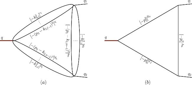
Figure 3. (a) The massless three-point multi-edge graph. The number of loop is m + n + l − 2, where m, n, l, are the number of edges at each side respectively. (b) The reduced graph after using equation ( |
By setting the indexes a1, b1, c1 equal to 1, other indexes equal to 2, we obtain the UT basis as well as the corresponding ε-expansion 33 ) up to three-loop order is
$\begin{eqnarray}\begin{array}{rcl} & & {I}_{3}^{(m+n+l-2)}\left(q,\{1,\mathop{\underbrace{2,\ldots ,2}}\limits_{m-1}\},\{1,\mathop{\underbrace{2,\ldots ,2}}\limits_{n-1}\},\{1,\mathop{\underbrace{2,\ldots ,2}}\limits_{l-1}\}\right)\\ & & \quad =\frac{{\rm{\Gamma }}{(1-\epsilon )}^{3}{\rm{\Gamma }}{(-\epsilon )}^{l+m+n-3}}{{(-{q}^{2})}^{1+(m+n+l-2)\epsilon }}\\ & & \qquad \times \,\frac{{\rm{\Gamma }}(1+(m-1)\epsilon ){\rm{\Gamma }}((1-m-n)\epsilon ){\rm{\Gamma }}((1-m-l)\epsilon ){\rm{\Gamma }}(1+(m+n+l-2)\epsilon )}{{\rm{\Gamma }}(1-m\epsilon ){\rm{\Gamma }}(1-n\epsilon ){\rm{\Gamma }}(1-l\epsilon ){\rm{\Gamma }}(1-(m+n+l-1)\epsilon )}.\end{array}\end{eqnarray}$
The ε-expansion of equation ( $\begin{eqnarray}{\tilde{I}}_{3}^{(1+1+1-2)}=\frac{1}{{\epsilon }^{2}}-\frac{{\pi }^{2}}{12}-\frac{7\zeta (3)\epsilon }{3}-\frac{47{\pi }^{4}{\epsilon }^{2}}{1440}+O({\epsilon }^{3}),\end{eqnarray}$
$\begin{eqnarray}\begin{array}{rcl}{\tilde{I}}_{3}^{(2+1+1-2)} & = & -\frac{1}{4{\epsilon }^{3}}-\frac{{\pi }^{2}}{24\epsilon }+\frac{13\zeta (3)}{6}+\frac{41{\pi }^{4}\epsilon }{1440}\\ & & +\left[\frac{13{\pi }^{2}\zeta (3)}{36}+\frac{121\zeta (5)}{10}\right]{\epsilon }^{2}+O({\epsilon }^{3}),\end{array}\end{eqnarray}$
$\begin{eqnarray}\begin{array}{rcl}{\tilde{I}}_{3}^{(1+2+1-2)} & = & -\frac{1}{2{\epsilon }^{3}}+\frac{{\pi }^{2}}{12\epsilon }+\frac{16\zeta (3)}{3}+\frac{19{\pi }^{4}\epsilon }{240}\\ & & +\left[\frac{136\zeta (5)}{5}-\frac{8{\pi }^{2}\zeta (3)}{9}\right]{\epsilon }^{2}+O({\epsilon }^{3}),\end{array}\end{eqnarray}$
$\begin{eqnarray}\begin{array}{rcl}{\tilde{I}}_{3}^{(3+1+1-2)} & = & \frac{1}{9{\epsilon }^{4}}+\frac{{\pi }^{2}}{12{\epsilon }^{2}}-\frac{23\zeta (3)}{9\epsilon }+\frac{7{\pi }^{4}}{864}\\ & & +\left[-\frac{23{\pi }^{2}\zeta (3)}{12}-\frac{117\zeta (5)}{5}\right]\epsilon +\left[\frac{529\zeta {(3)}^{2}}{18}-\frac{65243{\pi }^{6}}{1088640}\right]{\epsilon }^{2}\\ & & +\,O({\epsilon }^{3}),\end{array}\end{eqnarray}$
$\begin{eqnarray}\begin{array}{rcl}{\tilde{I}}_{3}^{(1+3+1-2)} & = & \frac{1}{3{\epsilon }^{4}}-\frac{{\pi }^{2}}{12{\epsilon }^{2}}-\frac{29\zeta (3)}{3\epsilon }-\frac{71{\pi }^{4}}{480}\\ & & +\left[\frac{29{\pi }^{2}\zeta (3)}{12}-\frac{421\zeta (5)}{5}\right]\epsilon +\left[\frac{841\zeta {(3)}^{2}}{6}-\frac{11539{\pi }^{6}}{72576}\right]{\epsilon }^{2}\\ & & +O({\epsilon }^{3}),\end{array}\end{eqnarray}$
$\begin{eqnarray}\begin{array}{rcl}{\tilde{I}}_{3}^{(2+2+1-2)} & = & \frac{1}{6{\epsilon }^{4}}+\frac{{\pi }^{2}}{24{\epsilon }^{2}}-\frac{23\zeta (3)}{6\epsilon }-\frac{25{\pi }^{4}}{576}+\left[-\frac{23{\pi }^{2}\zeta (3)}{24}-\frac{351\zeta (5)}{10}\right]\epsilon +\left[\frac{529\zeta {(3)}^{2}}{12}-\frac{66041{\pi }^{6}}{725760}\right]{\epsilon }^{2}\\ & & +\,O({\epsilon }^{3}),\end{array}\end{eqnarray}$
$\begin{eqnarray}\begin{array}{rcl}{\tilde{I}}_{3}^{(1+2+2-2)}v & = & \frac{1}{4{\epsilon }^{4}}-\frac{{\pi }^{2}}{16{\epsilon }^{2}}-\frac{29\zeta (3)}{4\epsilon }-\frac{71{\pi }^{4}}{640}\\ & & +\left[\frac{29{\pi }^{2}\zeta (3)}{16}-\frac{1263\zeta (5)}{20}\right]\epsilon +\left[\frac{841\zeta {(3)}^{2}}{8}-\frac{11539{\pi }^{6}}{96768}\right]{\epsilon }^{2}\\ & & +\,O({\epsilon }^{3}).\end{array}\end{eqnarray}$
Here, for brevity, we introduce the notation ${\tilde{I}}_{3}^{(m+n+l-2)}={\,\rm{e}\,}^{(m+n+l-2){\gamma }_{\,\rm{E}\,}\epsilon }{(-{q}^{2})}^{1+(m+n+l-2)\epsilon }\,\times {I}_{3}^{(m+n+l-2)}(q,\{1,2,\ldots ,2\},\{1,2,\ldots ,2\},\{1,2,\ldots ,2\})$.5. Generalize to massless N-point multi-edge integral
The calculations in sections 3 and 4 are based on the fact that the massless banana can be integrated out and result in a shift on the power of the propagator. This technique can be used to simplify any integral with the substructure of a massless banana. Considering the massless N-point multi-edge integral shown in figure 4(a). The external momenta are denoted by qi, with overall momentum conservation ${\sum }_{i=1}^{N}{q}_{i}=0$; the loop momenta are denoted by k0, ki,j; the number of edges of the ith side is indicated with ni, and hence the loop number is $1+{\sum }_{i=1}^{N}({n}_{i}-1)$. Like the three-point case in section 4 , this N-point multi-edge integral finally reduces to an one-loop integral with non-integer propagator power, as shown in figure 4(b). The corresponding formula reads
$\begin{eqnarray}\begin{array}{rcl} & & {I}_{N}^{(1+\displaystyle \sum _{i=1}^{N}({n}_{i}-1))}\left(\{{Q}_{i}\},\{{a}_{1,i}\},\cdots \,,\{{a}_{N,i}\}\right)\\ & & \quad =\,\displaystyle \prod _{i=1}^{N}\left[\frac{{\rm{\Gamma }}({A}_{i,{n}_{i}})}{{\rm{\Gamma }}\left(\frac{d}{2}-{A}_{i,{n}_{i}}\right)}\displaystyle \prod _{j=1}^{{n}_{i}}\frac{{\rm{\Gamma }}\left(\frac{d}{2}-{a}_{i,j}\right)}{{\rm{\Gamma }}({a}_{i,j})}\right]\\ & & \times \,\displaystyle \int \frac{{\,\rm{d}\,}^{d}{k}_{0}}{i{\pi }^{d/2}}\frac{1}{{[-{k}_{0}^{2}]}^{{A}_{1,{n}_{1}}}{[-{({k}_{0}-{q}_{1})}^{2}]}^{{A}_{2,{n}_{2}}}\cdots {\left[-{\left({k}_{0}-\displaystyle \sum _{i=1}^{N-1}{q}_{i}\right)}^{2}\right]}^{{A}_{N,{n}_{N}}}},\end{array}\end{eqnarray}$
where Qi denote the external momentum scales, ${A}_{i,{n}_{i}}\,={\sum }_{j=1}^{{n}_{i}}({a}_{i,j}-\frac{d}{2})+\frac{d}{2}$. Generally speaking, evaluating a one-loop integral with general propagator powers is not as simple as evaluating standard one-loop integral (where all propagator powers are unity). Fortunately, there has been much research made around this topic [28–31]. Collectively, these prior studies, together with our present work and the method of differential equations, establish a comprehensive framework for addressing a broader class of integrals possessing the massless banana substructure.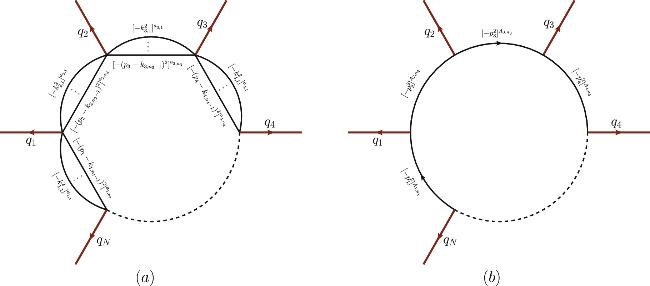
Figure 4. (a) The massless N-point multi-edge graph. The number of loop is $1+{\sum }_{i=1}^{N}({n}_{i}-1)$, where ni are the number of edges of the ith side. (b) The reduced graph after using equation ( |
6. Discussions and conclusion
In this paper, we present the analytic results for three classes of Feynman integrals, including the massless banana integral, the one-mass banana integral, and the massless three-point multi-edge integral. By combining the recursive property of the massless two-point integral, with the previous research on one-loop integrals with arbitrary propagator powers, we obtain the analytic results at any loop order. It turns out that the results are quite simple and compact, especially after choosing basis with uniform transcendentality. The calculation method used in this work is straightforward, and can be generalized to general cases where the massless propagator is “dressed” by a massless banana, we leave these topics to future works.
The analytic results in this work may also serve as boundary conditions for more complicated integrals. For phenomenology applications, the integrals in this work will contribute to the high order corrections of many interesting phenomena, like the heavy quarks production and decay, and the massless quark and gluon form factors. The banana integrals we discussed can also be used for the calculation of multi-particle phase space integrals including a massive particle.