


1. Introduction
Nonlinear circuits have garnered attention for their ability to mimic the dynamic behaviors of complex biological systems [1–3]. They are particularly adept at replicating the nonlinear characteristics and dynamic actions of biological systems when simulating neurons and muscle cells. By combining electronic components, circuit models can be constructed that emulate the electrical behavior of biological cells [4–7]. These models are capable of simulating various states of neurons, including resting states, spike firing states, burst firing states, and even chaotic firing states [8–10]. Within nonlinear circuits, inductance and magnetic flux-controlled memristors (MFCMs) can simulate the induced currents or magnetic flux in neurons. These variables are instrumental in studying the effects of magnetic fields on ion channel currents, thereby influencing the excitability of neurons [11–13]. In exploring the mechanisms of neuronal firing and their role in neurological diseases, scientists have constructed complex mathematical models to simulate neuronal behavior [14–17]. For instance, based on the Hindmarsh–Rose neuron model, researchers have considered the effects of magnetic flux and electromagnetic induction on the cell membrane, constructing a four-dimensional model [18]. Through interspike interval bifurcation diagrams, they found that the model can produce complex dynamic phenomena, including reverse period-doubling bifurcations, reverse fold bifurcations, and period-doubling bifurcations leading to chaos, which helps us understand the complexity of abnormal neuronal firing [12, 19, 20]. The application of memristors in neuronal circuits is multifaceted; they cannot only simulate the plasticity of neural synapses but also control hidden firing phenomena [21, 22]. Hidden firing refers to the non-manifest discharge behavior exhibited by the system under certain parameter conditions. By designing specific controllers, the dynamic characteristics of neuronal circuits can be altered, thereby eliminating undesired hidden firing phenomena, which is of great significance for understanding neurological diseases [23]. Furthermore, memristors can be coupled with phototubes to construct neuron circuits sensitive to light signals. Such circuits can simulate the response of biological neurons to light stimuli, further exploring the functions and mechanisms of the nervous system [24–26]. With the advancement of electronic technology, the emergence of new electronic components such as memristors has provided more possibilities for the simulation of nonlinear circuits [27–29]. The nonlinear characteristics of memristors give them a unique advantage in simulating biological nervous systems. Josephson junctions can be used to construct highly sensitive sensors to detect subtle changes in magnetic fields, which can then be used to analyze the tiny electromagnetic field changes in neural activity [30–33]. These studies have not only promoted the development of nonlinear circuit design but also provided new perspectives for understanding the complex behavior of the nervous system. Through these simulation systems, scientists can delve deeper into the mechanisms of abnormal neuronal firing and how such abnormal discharges can lead to brain diseases, such as epilepsy and Parkinson’s disease [34–36].
In the biological nervous system, the interaction between neurons and skeletal muscle cells is fundamental to the realization of motor control and force generation [37]. The complexity of this interaction is not only reflected in the signal transmission between cells but also involves the intricate biophysics within the cells themselves [38]. This intricate relationship is crucial for understanding how the nervous system regulates muscle activity, leading to movement and the generation of force [39]. The study of these interactions is vital for developing therapeutic strategies for neurological and muscular disorders and enhancing our knowledge of the basic principles of neuromuscular communication. The movement of muscles driven by neurons forms the foundation of how the nervous system controls bodily movements. Under normal conditions, the brain releases signals through motor neurons to trigger muscle contractions and movements [40]. To simulate this natural process, researchers have employed a variety of technical methods. For instance, using Neuromuscular Electrical Stimulation (NMES) technology, muscle contractions can be activated, thereby controlling the motion of robotic arms [41]. Furthermore, investigators have developed computational models to simulate the dynamics of musculoskeletal systems and the control mechanisms of neuromuscular activity [42]. These models are capable of predicting new movement patterns. Specifically, researchers such as Ngongiah et al [39] found through stability analysis that a single mechanical arm driven by a Josephson junction circuit would have two equilibrium points at certain stimulus current values, switching stability between these points. Yamapi et al [43] analyzed a small network that included three unidirectionally coupled Rayleigh–Duffing oscillators in a ring configuration. Meanwhile, Mbeunga et al [44] analyzed the dynamics of one single Fitzhugh–Nagumo (FHN) neuron coupled to a mechanical arm, and the oscillation boundaries are provided. In this article, we introduce an equivalent neural circuit model and simulate the neuromuscular junction using memristors, achieving the coupling of the neural circuit with the skeletal muscle cell circuit. We further explore the dynamic characteristics of this coupled system under various parameter settings.
2. Model and scheme
In this study, a neuron simulation circuit is constructed by integrating fundamental physical components, including resistors, capacitors, inductors, voltage sources, and nonlinear resistors, as depicted in figure 1(a). To emulate the biophysical properties of skeletal muscle cells, capacitors, inductors, and an electromagnetically driven mechanical system are paralleled, with the specific configuration shown in figure 1(b). Furthermore, memristors are employed as coupling synapses to facilitate the transmission of information and the exchange of energy between the neuron circuit and the skeletal muscle cell model.
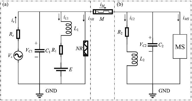
Figure 1. Equivalent circuit diagram of (a) neuron and (b) skeletal muscle cell connected by memristive synapses. |
In figure 1(a), VC1 and iL represent the equivalent membrane potential and the recovery variable of the neuron’s slow current, respectively. Vs denotes the voltage change induced by external stimulation, which can regulate the activities of the neuronal potential VC1 and the channel current iL. NR and M denote the nonlinear resistor and memristor, respectively. The currents through the memristor and the nonlinear resistor [12] can be expressed as:
$\begin{eqnarray}\left\{\begin{array}{l}{i}_{M}=f({\rm{\Phi }})=\frac{{\rm{d}}q({\rm{\Phi }})}{{\rm{d}}t}=\frac{{\rm{d}}q({\rm{\Phi }})}{{\rm{d}}{\rm{\Phi }}}\frac{{\rm{d}}{\rm{\Phi }}}{{\rm{d}}t}=w({\rm{\Phi }})({V}_{C1}-{V}_{C2})={\lambda }_{M}({\alpha }^{{\prime} }+3{\beta }^{{\prime} }{{\rm{\Phi }}}^{2})({V}_{C1}-{V}_{C2}),\\ {i}_{NR}=g({V}_{C1})=-\frac{1}{\rho }({V}_{C1}-\frac{1}{3}\frac{{V}_{C1}^{3}}{{V}_{0}^{2}}).\end{array}\right.\end{eqnarray}$
where f(Φ) is the current-voltage characteristic function of the nonlinear resistor, where iM represents the current through the memristor. And g(VC1) is the current-voltage characteristic function of the memristor. The functions f(Φ) and g(VC1) typically have nonlinear properties, capable of simulating the complex dynamic behavior of neurons. The nonlinear resistor is used to simulate the nonlinear characteristics of the neuronal membrane potential, while the memristor is used to simulate the synaptic plasticity between neurons. The parameter λm denotes the coupling strength of the memristor when acting as a coupling channel, Φ represents the magnetic flux of the memristor, q represents the charge, another intrinsic parameter determined by the structure of the memristor, and $({\alpha }^{{\prime} },{\beta }^{{\prime} })$ are the intrinsic parameters of the memristor. ρ and V0 denote the equivalent conductance and reverse cut-off voltage of the nonlinear resistor, respectively. In figure 1(b) the capacitor C2 is used to represent the membrane potential of the muscle cell. The L2 represents the inductance associated with the ion channels in the muscle cell. The R2 is used to model the thermal effect in the muscle cell. Based on Kirchhoff’s laws, the current-voltage analysis of the circuit depicted in figure 1 can be conducted to determine the operational characteristics of the circuit. This analysis involves the following steps $\begin{eqnarray}\left\{\begin{array}{l}{C}_{1}\frac{{\rm{d}}{V}_{C1}}{{\rm{d}}t}=\frac{{V}_{S}-{V}_{C1}}{{R}_{S}}-{i}_{L1}-{i}_{NR}-{i}_{M},\\ {L}_{1}\frac{{\rm{d}}{i}_{L1}}{{\rm{d}}t}={V}_{C1}+E-{R}_{1}{i}_{L1},\\ \frac{{\rm{d}}{\rm{\Phi }}}{{\rm{d}}t}={V}_{C1}-{V}_{C2},\\ {C}_{2}\frac{{\rm{d}}{V}_{C2}}{{\rm{d}}t}={i}_{M}-{i}_{L2}-{i}_{MS},\\ {L}_{2}\frac{{\rm{d}}{i}_{L2}}{{\rm{d}}t}={V}_{C2}-{R}_{2}{i}_{L2},\\ {L}_{MS}\frac{{\rm{d}}{i}_{MS}}{{\rm{d}}t}={V}_{C2}-{R}_{MS}{i}_{MS}-Bl\frac{{\rm{d}}\chi }{{\rm{d}}t}.\end{array}\right.\end{eqnarray}$
In equation (2 ), VC2 and iL2 represent the membrane potential and channel current in the skeletal muscle cell model, respectively. In the MS structure, the inductance and resistance of the windings are denoted by LMS and RMS, respectively, while iMS represents the current flowing through these windings. The length ℓ of the winding wire. Bℓdχ/dt denotes the induced voltage generated within the windings. During coordinated movement in animals, a relative sliding occurs between the myosin and actin within the skeletal muscle cells, and this biophysical process is simulated by the mechanical device shown in figure 2.
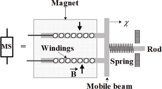
Figure 2. Schematic diagram of the internal structure of an electromagnetically driven robotic arm. |
Kitio et al conducted an in-depth study on a class of self-sustained macroscopic electromagnetic mechanical systems (MaEMS) and successfully constructed corresponding experimental models. They not only conducted a meticulous stability analysis of these models but also went on to design the corresponding device models [45, 46]. Mbeunga et al focused on MaEMS arrays driven by FHN neurons and provided a comprehensive analysis of their dynamic characteristics [44]. Inside the MS device, a uniform magnetic field is present. The time-varying current output from the neuron is fed into the winding within the MS. When the current-carrying conductor is placed in the magnetic field, it experience a magnetic force on this conductor. Since the winding is fixed to the beam, this force simultaneously drives the winding and the beam. This, in turn, actuates the movement of the mechanical arm. Building on these studies, we can derive the motion equation for a moving beam with mass m, which is expressed as follows
$\begin{eqnarray}\left\{\begin{array}{l}\frac{{\rm{d}}\chi }{{\rm{d}}t}=v,\\ m\frac{{\rm{d}}v}{{\rm{d}}t}+{\beta }_{0}v+K\chi =Bl{i}_{MS}.\end{array}\right.\end{eqnarray}$
The displacement of the moving beam is denoted by χ, and its velocity during motion is represented by v. β0 represents the damping coefficient of the moving beam during its motion, K denotes the stiffness coefficient of the spring, ℓ is the total length of the conductor used in the winding, and the term BℓiMS represents the Ampere force experienced by the conductor in the magnetic field. For the convenience of research, the following dimensionless variable substitutions are made for the physical quantities in equations (1 ), (2 ), and (3 ),
$\begin{eqnarray}\left\{\begin{array}{l}x=\frac{{V}_{C1}}{{V}_{0}},\xi =\frac{\rho }{{R}_{S}},{u}_{S}=\frac{{V}_{S}}{{V}_{0}},\alpha ={\alpha }^{{\prime} }\rho ,\beta ={\beta }^{{\prime} }{\rho }^{3}{C}_{1}^{2}{V}_{0}^{2},\\ y=\frac{\rho {i}_{L1}}{{V}_{0}},a=\frac{E}{{V}_{0}},b=\frac{{R}_{1}}{\rho },c=\frac{{\rho }^{2}{C}_{1}}{{L}_{1}},\varphi =\frac{{\rm{\Phi }}}{\rho {C}_{1}{V}_{0}},\tau =\frac{t}{\rho {C}_{1}},\\ {x}_{1}=\frac{{V}_{C2}}{{V}_{0}},\gamma =\frac{{C}_{1}}{{C}_{2}},{y}_{1}=\frac{\rho {i}_{L2}}{{V}_{0}},{\eta }_{1}=\frac{{\rho }^{2}{C}_{1}}{{L}_{2}},{\eta }_{2}=\frac{\rho {R}_{2}{C}_{1}}{{L}_{2}},\\ z=\frac{\rho {i}_{MS}}{{V}_{0}},{k}_{1}=\frac{{\rho }^{2}{C}_{1}}{{L}_{MS}},{k}_{2}=\frac{{R}_{MS}\rho {C}_{1}}{{L}_{MS}},{k}_{3}=\frac{B{l}^{2}\rho }{{V}_{0}{L}_{MS}},\\ h=\frac{\chi }{l},{v}^{{\prime} }=\frac{v\rho {C}_{1}}{l},{m}_{1}=\frac{\rho {C}_{1}^{2}{V}_{0}B}{m},{m}_{2}=\frac{{C}_{1}\rho {\beta }_{0}}{m},{m}_{3}=\frac{{\rho }^{2}{C}_{1}^{2}K}{m}.\end{array}\right.\end{eqnarray}$
The dimensionless equations for the system shown in figure 1 can be expressed as
$\begin{eqnarray}\left\{\begin{array}{l}\frac{{\rm{d}}x}{{\rm{d}}\tau }=x(1-\xi )-\frac{1}{3}{x}^{3}-y+\xi {u}_{S}-{\lambda }_{M}(\alpha +3\beta {\varphi }^{2})(x-{x}_{1}),\\ \frac{{\rm{d}}y}{{\rm{d}}\tau }=c(x-by+a),\\ \frac{{\rm{d}}\varphi }{{\rm{d}}\tau }=x-{x}_{1},\\ \frac{{\rm{d}}{x}_{1}}{{\rm{d}}\tau }=\gamma \left[{\lambda }_{M}(\alpha +3\beta {\varphi }^{2})(x-{x}_{1})-{y}_{1}-z\right],\\ \frac{{\rm{d}}{y}_{1}}{{\rm{d}}\tau }={\eta }_{1}{x}_{1}-{\eta }_{2}{y}_{1}{\rm{,}}\\ \frac{{\rm{d}}z}{{\rm{d}}\tau }={k}_{1}{x}_{1}-{k}_{2}z-{k}_{3}{v}^{{\prime} },\\ \frac{{\rm{d}}h}{{\rm{d}}\tau }={v}^{{\prime} },\\ \frac{{\rm{d}}{v}^{{\prime} }}{{\rm{d}}\tau }={m}_{1}z-{m}_{2}{v}^{{\prime} }-{m}_{3}h.\end{array}\right.\end{eqnarray}$
Similar to traditional circuits, the electrical field energy in neuron circuits and skeletal muscle cell circuits is stored in capacitors, while the magnetic field energy is stored within inductors. Furthermore, when skeletal muscle cells are active, their dynamically varying energy also includes the kinetic energy of the moving beams and the elastic potential energy of the springs. These two components of energy reflect the changes in kinetic and potential energy over time as actin and myosin undergo relative motion. Additionally, memristors possess the characteristic of storing magnetic field energy. Therefore, we can delineate the energy of neuron circuits, skeletal muscle cell circuits, and memristive synapses respectively,
$\begin{eqnarray}\left\{\begin{array}{c}{W}_{S}={W}_{N}+{W}_{M}+{W}_{Mu},{H}_{S}={H}_{N}+{H}_{M}+{H}_{Mu},\\ {W}_{N}=\frac{1}{2}{C}_{1}{V}_{C1}^{2}+\frac{1}{2}{L}_{1}{i}_{L1}^{2},{W}_{M}=\frac{1}{2}{\rm{\Phi }}{i}_{M},\\ {W}_{Mu}=\frac{1}{2}{C}_{2}{V}_{C2}^{2}+\frac{1}{2}{L}_{2}{i}_{L2}^{2}+\frac{1}{2}{L}_{MS}{i}_{MS}^{2}-\frac{1}{2}K{\chi }^{2}+\frac{1}{2}m{v}^{2},\\ {H}_{N}=\frac{1}{2}{x}^{2}+\frac{1}{2c}{y}^{2},{H}_{M}=\frac{1}{2}{\lambda }_{M}(\alpha \varphi +3\beta {\varphi }^{3})(x-{x}^{{\prime} }),\\ {H}_{Mu}=\frac{1}{2\gamma }{x{}^{{\prime} }}^{2}+\frac{1}{2{\eta }_{1}}{y{}^{{\prime} }}^{2}+\frac{1}{2{k}_{1}}{z}^{2}-\frac{1}{2{m}_{4}}{h}^{2}+\frac{1}{2{m}_{5}}{v{}^{{\prime} }}^{2},\\ {H}_{S}=\frac{1}{2}{x}^{2}+\frac{1}{2c}{y}^{2}+\frac{1}{2}{\lambda }_{M}(\alpha \varphi +3\beta {\varphi }^{3})(x-{x}^{{\prime} })+\\ \frac{1}{2\gamma }{x{}^{{\prime} }}^{2}+\frac{1}{2{\eta }_{1}}{y{}^{{\prime} }}^{2}+\frac{1}{2{k}_{1}}{z}^{2}-\frac{1}{2{m}_{4}}{h}^{2}+\frac{1}{2{m}_{5}}{v{}^{{\prime} }}^{2}.\end{array}\right.\end{eqnarray}$
Here, ${m}_{4}={C}_{1}{V}_{0}^{2}/K{\ell }^{2}$, ${m}_{5}={\rho }^{2}{C}_{1}^{3}{V}_{0}^{2}/m{\ell }^{2}={m}_{3}* {m}_{4}$. WS and HS represent the dimensionless representation of the neuron circuit and skeletal muscle cell circuit coupled by memristive synapses, respectively. WN and HN are used to describe the physical field energy and Hamiltonian of the neuron circuit. WM and HM represent the field energy in the memristor channel and its dimensionless expression, respectively. WMu and HMu define the physical energy and dimensionless expression of the skeletal muscle cell circuit, respectively. The kinetic energy of the moving beam is given by Ek = mv2/2, and the elastic potential energy of the spring is represented by Kχ2/2, with their dimensionless expressions denoted as ${H}_{EK}={v{}^{{\prime} }}^{2}/2{m}_{5}$ and h2/2m4, respectively. According to Helmholtz’s theorem [47], a single skeletal muscle cell in equation (5 ) can be written in an equivalent vector form that includes a dissipative field Fc(X) and a conservative field Fd(X), as shown below
$\begin{eqnarray}\left\{\begin{array}{l}\frac{{\rm{d}}X}{{\rm{d}}\tau }={F}_{c}(X)+{F}_{d}(X),X\subset {R}^{N},\\ {\rm{\nabla }}{H}^{T}{F}_{c}(X)=0,\\ {\rm{\nabla }}{H}^{T}{F}_{d}(X)=\mathop{H}\limits^{.}=\frac{{\rm{dH}}}{{\rm{d}}\tau },\end{array}\right.\end{eqnarray}$
where X represents the set of all variables of the system under analysis, that is, X = {x, y, …}, μ denotes the set of normalized parameters, that is, μ = {γ, η1, η2, k1, k2, k3, m1, m2, m3, m4, m5}, and H denotes the Hamiltonian energy function of a single system. The superscript T refers to the transpose operation of the energy function matrix. The Helmholtz theorem is used to verify the electromagnetic field, and the Hamiltonian energy in figure 1 can be expressed as $\begin{eqnarray}\begin{array}{l}H={x}^{2}/2+{y}^{2}/2c+{\lambda }_{M}(\alpha \varphi +3\beta {\varphi }^{3})\\ \,\times \,(x-{x}_{1})/2+{x}_{1}^{2}/2\gamma +{y}_{1}^{2}/2{\eta }_{1}+{z}^{2}/2{k}_{1}.\end{array}\end{eqnarray}$
The mechanical energy was removed from the total energy of skeletal muscle, and the velocity and displacement equations were eliminated from equation (5 ), which was then decomposed as follows11 ) is consistent with the expression shown in equation (6 ).
$\begin{eqnarray*}\begin{array}{l}\left[\begin{array}{l}\frac{{\rm{d}}x}{{\rm{d}}\tau }\\ \frac{{\rm{d}}y}{{\rm{d}}\tau }\\ \frac{{\rm{d}}\varphi }{{\rm{d}}\tau }\\ \frac{{\rm{d}}{x}_{1}}{{\rm{d}}\tau }\\ \frac{{\rm{d}}{y}_{{\rm{1}}}}{{\rm{d}}\tau }\\ \frac{{\rm{d}}z}{{\rm{d}}\tau }\end{array}\right]\,=\,\left[\begin{array}{l}x(1-\xi )-\frac{1}{3}{x}^{3}-y+\xi {u}_{S}-{\lambda }_{M}(\alpha +3\beta {\varphi }^{2})(x-{x}_{1})\\ c(x-by+a)\\ x-{x}_{1}\\ \gamma [{I}_{ext}-{y}_{1}-z]\\ {\eta }_{1}{x}_{1}-{\eta }_{2}{y}_{1}\\ {k}_{1}{x}_{1}-{k}_{2}z-{k}_{3}{v}^{{\prime} }\end{array}\right]\\ =\,{F}_{c}+{F}_{d}\\ =\,\left[\begin{array}{c}-y\\ cx+\frac{1}{2}c{\lambda }_{M}\left(\alpha \varphi +3\beta {\varphi }^{3}\right)\\ 0\\ -{y}_{1}\\ \frac{{\eta }_{1}{x}_{1}}{\gamma }-\frac{1}{2}{\eta }_{1}{\lambda }_{M}\left(\alpha \varphi +3\beta {\varphi }^{3}\right)\\ 0\end{array}\right]\\ +\,\left[\begin{array}{l}x(1-\xi )-\frac{1}{3}{x}^{3}+\xi {u}_{S}-{\lambda }_{M}(\alpha +3\beta {\varphi }^{2})(x-{x}_{1})\\ c(-by+a)-\frac{1}{2}c{\lambda }_{M}\left(\alpha \varphi +3\beta {\varphi }^{3}\right)\\ x-{x}_{1}\\ \gamma [{I}_{ext}-{y}_{1}-z]+{y}_{1}\\ {\eta }_{1}{x}_{1}-{\eta }_{2}{y}_{1}-\frac{{\eta }_{1}}{\gamma }{x}_{1}+\frac{1}{2}{\eta }_{1}{\lambda }_{M}\left(\alpha \varphi +3\beta {\varphi }^{3}\right)\\ {k}_{1}{x}_{1}-{k}_{2}z-{k}_{3}{v}^{{\prime} }\end{array}\right]\end{array}\end{eqnarray*}$
$\begin{eqnarray}\begin{array}{l}=\left[\begin{array}{cccccc}0 & -c & 0 & 0 & 0 & 0\\ c & 0 & 0 & 0 & 0 & 0\\ 0 & 0 & 0 & 0 & 0 & 0\\ 0 & 0 & 0 & 0 & -{\eta }_{1} & 0\\ 0 & 0 & 0 & {\eta }_{1} & 0 & 0\\ 0 & 0 & 0 & 0 & 0 & 0\\ \end{array}\right]\left[\begin{array}{c}x+\frac{1}{2}{\lambda }_{M}\left(\alpha \varphi +3\beta {\varphi }^{3}\right)\\ \frac{y}{c}\\ \frac{1}{2}{\lambda }_{M}(\alpha +9\beta {\varphi }^{2})(x-{x}_{1})\\ \frac{{x}_{1}}{\gamma }-\frac{1}{2}{\lambda }_{M}\left(\alpha \varphi +3\beta {\varphi }^{3}\right)\\ \frac{{y}_{1}}{{\eta }_{1}}\\ \frac{z}{{k}_{1}}\end{array}\right]\\ +\left[\begin{array}{cccccc}{a}_{11} & 0 & 0 & 0 & 0 & 0\\ 0 & {a}_{22} & 0 & 0 & 0 & 0\\ 0 & 0 & {a}_{33} & 0 & 0 & 0\\ 0 & 0 & 0 & {a}_{44} & 0 & 0\\ 0 & 0 & 0 & 0 & {a}_{55} & 0\\ 0 & 0 & 0 & 0 & 0 & {a}_{66}\end{array}\right]\left[\begin{array}{c}x+\frac{1}{2}{\lambda }_{M}\left(\alpha \varphi +3\beta {\varphi }^{3}\right)\\ \frac{y}{c}\\ \frac{1}{2}{\lambda }_{M}(\alpha +9\beta {\varphi }^{2})(x-{x}_{1})\\ \frac{{x}_{1}}{\gamma }-\frac{1}{2}{\lambda }_{M}\left(\alpha \varphi +3\beta {\varphi }^{3}\right)\\ \frac{{y}_{1}}{{\eta }_{1}}\\ \frac{z}{{k}_{1}}\end{array}\right].\end{array}\end{eqnarray}$
In the given context, with parameter $\begin{eqnarray}\left\{\begin{array}{l}{a}_{11}=\left[x\left(1-\xi \right)-{x}^{3}/3+\xi {u}_{S}-{\lambda }_{M}\left(\alpha +3\beta {\varphi }^{2}\right)\left(x-{x}_{1}\right)\right]/\left[x+0.5{\lambda }_{M}\left(\alpha \varphi +3\beta {\varphi }^{3}\right)\right],\\ {a}_{22}={c}^{2}\left[\left(-by+a\right)-0.5{\lambda }_{M}\left(\alpha \varphi +3\beta {\varphi }^{3}\right)\right]/y,\\ {a}_{33}=2/\left[{\lambda }_{M}\left(\alpha +9\beta {\varphi }^{2}\right)\right],\\ {a}_{44}=\left[\gamma \left({I}_{ext}-{y}_{1}-z\right)+{y}_{1}\right]/\left[{x}_{1}/\gamma -0.5{\lambda }_{M}\left(\alpha \varphi +3\beta {\varphi }^{3}\right)\right],\\ {a}_{55}={\eta }_{1}\left[{\eta }_{1}{x}_{1}-{\eta }_{2}{y}_{1}-{\eta }_{1}{x}_{1}/\gamma \right]+0.5{\lambda }_{M}{\eta }_{1}^{2}\left(\alpha \varphi +3\beta {\varphi }^{3}\right)/{y}_{1},\\ {a}_{66}=\left[{k}_{1}\left({k}_{1}{x}_{1}-{k}_{2}z-{k}_{3}{v}^{{\prime} }\right)\right]/z.\end{array}\right.\end{eqnarray}$
The Hamiltonian energy function of the mechanical system satisfies the following equation $\begin{eqnarray}\begin{array}{l}{\rm{\nabla }}{H}_{Mu}^{{\rm{T}}}{F}_{c}(X)=-y\frac{\partial H}{\partial x}\\ +\left[cx+\frac{1}{2}c{\lambda }_{M}\left(\alpha \varphi +3\beta {\varphi }^{3}\right)\right]\\ \,\,\times \,\frac{\partial H}{\partial y}+0* \frac{\partial H}{\partial \varphi }-{y}_{1}\frac{\partial H}{\partial {x}_{1}}\\ +\left[\frac{{\eta }_{1}{x}_{1}}{\gamma }-\frac{1}{2}{\eta }_{1}{\lambda }_{M}\left(\alpha \varphi +3\beta {\varphi }^{3}\right)\right]\\ \,\,\times \,\frac{\partial H}{\partial {y}_{1}}+0* \frac{\partial H}{\partial z}=0.\end{array}\end{eqnarray}$
The Hamiltonian energy obtained by solving equation (In practical scenarios, the exchange of information and energy between neurons is facilitated through the establishment of coupled synapses. Such synapses typically form between two neurons with different energy states, and their coupling strength increases exponentially over time until the energy difference between them is reduced below a certain threshold. Neurons and skeletal muscle cells are different types of cells, and achieving complete energy equilibrium when coupled as heterogeneous cells is challenging. It is widely believed that the strength of synaptic coupling between cells is closely related to their energy states. Therefore, this article uses the energy ratio between skeletal muscle cells and neuronal cells as the key factor for triggering synapse growth between them, and defines the expression of coupling strength in equation (12 )
$\begin{eqnarray}\frac{{\rm{d}}{\lambda }_{M}}{{\rm{d}}\tau }=\sigma {\lambda }_{M}K\Space{0ex}{0.25ex}{0ex}(\left|\frac{{H}_{Mu}}{{H}_{N}}\right|-\varepsilon \Space{0ex}{0.25ex}{0ex}).\end{eqnarray}$
Here, the step function K(∣HMμ/Hn∣ − ϵ) serves to cap the growth of coupling strength at a predetermined saturation point. The parameter σ, acting as the gain factor for coupling strength, is a positive constant. Once the energy ratio between skeletal muscle cells and neuronal cells surpasses a specific threshold, the coupling channel is activated, allowing for a further enhancement of coupling strength.3. Numerical results and discussion
In this section, the fourth-order Runge–Kutta algorithm is employed to compute the numerical solutions of the memristor-coupled neural circuit and the equivalent circuit of skeletal muscle cells. The time step is set to h = 0.01. Initially, the dynamic behavior of a single neuron is calculated with parameter values a = 0.7, b = 0.3, c = 0.4, and ξ = 0.175. The single neuron is subjected to an external stimulus generating a voltage ${\xi }_{u{\rm{s}}={I}_{0}+A{\rm{c}}{\rm{o}}{\rm{s}}\omega \tau }$. For the numerical modeling of the entire system, the parameter settings are as follows: a = 0.7, b = 0.3, c = 0.4, ξ = 0.175, I0 = 0.1, A = 0.4, λM = 0.1, α = 0.1, β = 0.1, γ = 1, η1 = 0.4, η2 = 0.12, k1 = 0.1, k2 = 0.1, k3 = 0.1, m1 = 0.1, m2 = 0.1, m3 = 0.1, m4 = 1, m5 = 0.1. By varying the angular frequency ω, different firing patterns of the neuron circuit are triggered. Figure 3 illustrates the distribution of the peak membrane potentials of a single neuron at various angular frequencies ω, as calculated from equation (5 ).
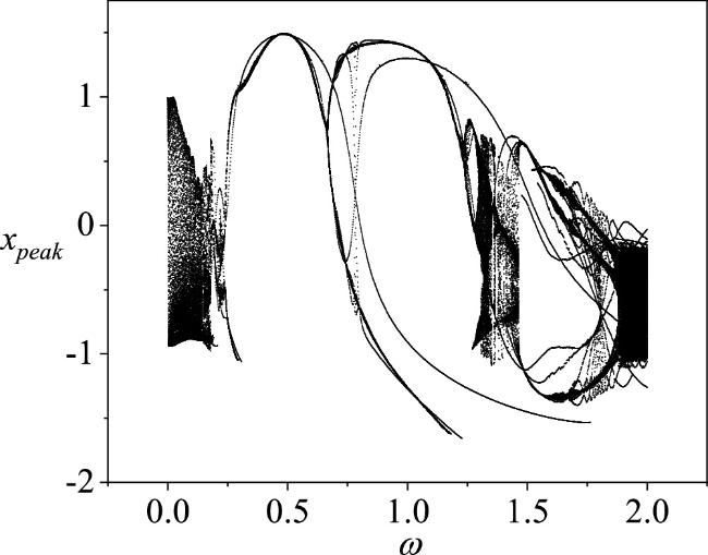
Figure 3. A bifurcation diagram of the membrane potential of a single neuron as the angular frequency ω varies, with the amplitude A set to 0.4. The parameters are chosen as a = 0.7, b = 0.3, c = 0.4, ξ = 0.175, I0 = 0.1. The initial conditions for the single neuron circuit are (0.2, 0.1). |
It is evident from figure 3 that by gradually adjusting the magnitude of the angular frequency ω in the voltage generated by the neuron in response to external stimuli, different firing patterns of the neuron can be induced. To further investigate the specific impact of the angular frequency ω on the neuron’s membrane potential, figure 4 demonstrates how neurons exhibit a variety of firing patterns under appropriate external stimulation. The angular frequency of the voltage induced by the external stimuli is set to different values.
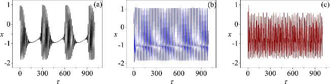
Figure 4. The patterns exhibited by an isolated neuron with different selections of angular frequency ω: (a) clustered firing at ω = 0.02; (b) spike firing at ω = 0.3; (c) chaotic firing at ω=1.3. Other parameters are held constant at a = 0.7, b = 0.3, c = 0.4, ξ = 0.175, I0 = 0.1, A = 0.4, with the initial conditions of the neuron circuit set to (0.2, 0.1). |
Figure 4 further confirms that changes in external stimuli can guide neurons into different states of excitation. Consequently, under external stimuli capable of generating various angular frequencies of voltage, a single neuron exhibits a range of firing patterns, including clustered firing, spiking firing, and chaotic firing. Moving forward, we will investigate the neuron circuit coupled by memristors and the skeletal muscle cell circuit. Based on equation (5 ), we have calculated the evolution of membrane potentials when the neuron circuit is coupled with the skeletal muscle cell circuit under clustered, spiking, and chaotic firing modes. This includes the attractors of the neuron circuit, the temporal variation of the membrane potential of the skeletal muscle cell, the attractors of the skeletal muscle cell circuit, the Hamiltonian energy ratio between the skeletal muscle cell circuit and the neuron circuit, the displacement of the active beam, the kinetic energy of the active beam, and the evolution of the field energy in the memristor-coupled channel over time. The parameters are set to a = 0.7, b = 0.3, c = 0.4, ξ = 0.175, I0 = 0.1, A = 0.4, λM = 0.1, α = 0.1, β = 0.1, γ = 1, η1 = 0.4, η2 = 0.12, k1 = 0.1, k2 = 0.1, k3 = 0.1, m1 = 0.1, m2 = 0.1, m3 = 0.1, m4 = 1, m5 = 0.1. By varying the angular frequency ω. The initial conditions for the coupled system are (0.2, 0.1, 0, 0.1, 0.1, 0.1, 0.1, 0.1), and the corresponding results are presented in figures 5, 6, and 7.
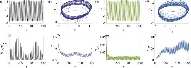
Figure 5. The dynamic behavior of a neuron circuit and a skeletal muscle cell circuit in a state of clustered firing, coupled via memristive synapses: (a) the variation in the neuron’s membrane potential; (b) the dynamics of the neuron circuit’s attractor; (c) the variation in the skeletal muscle cell’s membrane potential; (d) the dynamics of the skeletal muscle cell’s attractor; (e) the temporal evolution of the Hamiltonian energy ratio between the skeletal muscle cell and the neuron; (f) the temporal evolution of the displacement of the active beam; (g) the temporal evolution of the kinetic energy of the active beam; (h) the temporal evolution of the field energy in the memristor-coupled channel. In this analysis, the angular frequency is set to ω = 0.02. |
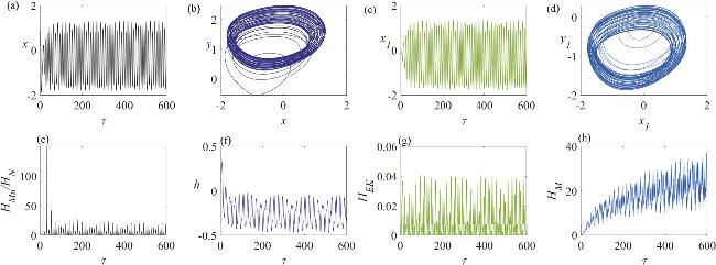
Figure 6. The dynamic characteristics of a neuron circuit and a skeletal muscle cell circuit in a spiking firing state, under the influence of memristive synapse coupling: (a) the variation in the neuron’s membrane potential; (b) the dynamics of the neuron circuit’s attractor; (c) the variation in the skeletal muscle cell’s membrane potential; (d) the dynamics of the skeletal muscle cell’s attractor; (e) the temporal evolution of the Hamiltonian energy ratio between the skeletal muscle cell and the neuron; (f) the temporal change in the displacement of the active beam; (g) the temporal variation in the kinetic energy of the active beam; (h) the temporal evolution of the field energy within the memristor-coupled channel. In this analysis, the angular frequency is set to ω = 0.3. |
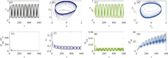
Figure 7. The dynamic characteristics of a neuron circuit and a skeletal muscle cell circuit in a chaotic firing state, under the influence of memristive synapse coupling: (a) the variation in the neuron’s membrane potential; (b) the dynamics of the neuron circuit’s attractor; (c) the variation in the skeletal muscle cell’s membrane potential; (d) the dynamics of the skeletal muscle cell’s attractor; (e) the temporal evolution of the Hamiltonian energy ratio between the skeletal muscle cell and the neuron; (f) the temporal change in the displacement of the active beam; (g) the temporal variation in the kinetic energy of the active beam; (h) the temporal evolution of the field energy within the memristor-coupled channel. In this analysis, the angular frequency is set to ω = 1.3. |
Figure 5 demonstrates the interaction between a neuron in a clustered firing state and a skeletal muscle cell, which is coupled via a memristor. A comparison between figures 4(a) and 5(a) reveals significant differences in the firing patterns of the neuron before and after coupling. The attractor diagram in figure 5(b) indicates that, under the current parameter settings, the neuron tends to fire periodically. The firing pattern of the skeletal muscle cell is similar to that of the neuron, a phenomenon attributed to the absence of nonlinear components in the skeletal muscle cell model, allowing the electrical activity of the neuron to directly and linearly affect the membrane potential and channel current of the skeletal muscle cell, as shown in figures 5(c) and (d). During the coupling process, the ratio of energy within the skeletal muscle cell to that within the neuron exceeds 1, suggesting that the average energy level of the skeletal muscle cell is higher than that of the neuron, as depicted in figure 5(e). The displacement variable h of the active beam oscillates periodically within a range of 0 to 0.5, as illustrated in figure 5(f). At the initial stage of coupling, the dimensionless kinetic energy of the active beam is relatively high, and as time progresses, its kinetic energy exhibits periodic changes within a smaller range, as shown in figure 5(g). Analysis of the expression for HM reveals that the value of HM is influenced by the intrinsic parameters of the memristor (α, β), the coupling strength of the coupling channel λM, the magnetic flux of the memristor φ, and the potential difference between the two cells. Further analysis of equation (5 ) indicates that the magnetic flux of the memristor is linearly related to the potential difference between the neuron and the skeletal muscle cell. Since the intrinsic parameters of the memristor do not evolve over time, the value of HM essentially depends on the potential difference between the two cells. Figure 5(h) shows that, as time evolves, HM exhibits an increasing trend, suggesting that the potential difference between the two cells is increasing and has not yet achieved potential synchronization.
Figure 6 illustrates the scenario where a neuron and a skeletal muscle cell in a spiking firing state are coupled through a memristor. By comparing figure 4(b) with figure 6(a), it is evident that coupling leads to significant changes in the neuron’s membrane potential. Specifically, under certain parameter settings, the neuron’s firing pattern exhibits characteristics of chaotic firing, which is reflected in the attractor diagram shown in figure 6(b). Concurrently, the membrane potential fluctuations of the skeletal muscle cell also demonstrate a trend towards chaotic evolution, as depicted in figures 6(c) and (d). Initially, at the onset of coupling, the Hamiltonian energy ratio between the skeletal muscle cell and the neuron has a large amplitude. However, as the coupling process continues, this energy ratio rapidly decreases and eventually oscillates within a specific range, as shown in figure 6(e). Furthermore, the displacement of the active beam exhibits a chaotic oscillation pattern over time, as illustrated in figure 6(f). The kinetic energy of the active beam consistently maintains chaotic oscillations within a certain range, as shown in figure 6(g). Figure 6(h) indicates that as time progresses, the magnetic field energy (HM) within the coupled channel shows an increasing trend, suggesting that the potential difference between the two cells is also gradually increasing. Throughout this process, the neuron and the skeletal muscle cell do not achieve potential synchronization.
Figure 7 illustrates the dynamic behavior of a neuron and a skeletal muscle cell in a chaotic firing state that are coupled through a memristor. By comparing figure 4(c) with figure 7(a), it can be observed that coupling leads to a transition from chaotic firing to periodic firing in the neuron. Concurrently, the membrane potential of the skeletal muscle cell also enters a state of periodic oscillation after coupling, as shown in figures 7(c) and (d). At the onset of coupling, the energy ratio between the skeletal muscle cell and the neuron is relatively high, but as the coupling progresses, this ratio gradually decreases, maintaining periodic oscillation within a specific range, as depicted in figure 7(e). Furthermore, the displacement of the active beam decreases over time and eventually stabilizes in a state of periodic oscillation, as illustrated in figure 7(f). The kinetic energy of the active beam also diminishes over time and then sustains periodic oscillation within a smaller range, as shown in figure 7(g). Figure 7(h) reveals an increasing trend in the magnetic field energy (HM) within the coupling channel over time, indicating that the potential difference between the two cells is gradually increasing, and throughout the entire experimental process, no potential synchronization is achieved between the neuron and the skeletal muscle cell. Based on the observations from figures 5, 6, and 7, it is evident that when neuron cells are coupled with skeletal muscle cells through memristive synapses, energy is transferred within the coupling channel. This coupling significantly alters the membrane potential of the neuron, which is markedly different from the uncoupled state. Moreover, under different oscillation states, the membrane potential of the skeletal muscle cell exhibits varying evolutionary patterns after coupling with the neuron, and the displacement of the active beam also demonstrates oscillations in different states over time. To gain a deeper understanding of the impact of memristive synapse coupling on neurons and skeletal muscle cells, a detailed analysis of the parameters related to the Hamiltonian energy of the skeletal muscle cell in the coupling system is carried out next. As indicated by equation (6 ), the Hamiltonian energy of the skeletal muscle cell is associated with the values of parameters (γ, η1, K1, m3). Initially, bifurcation diagrams and maximum Lyapunov exponent diagrams related to the capacitor parameter γ, which is associated with the equivalent membrane potential within the skeletal muscle cell, and the inductor parameter η1, which is related to the equivalent channel current, were calculated, with the results shown in figure 8.
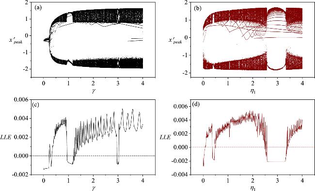
Figure 8. The bifurcation diagrams and maximum Lyapunov exponents for the variable direction parameters γ and η1 within the system where a neuron and a skeletal muscle cell are coupled via a memristor. In the diagrams, the parameters are assigned the following values: (a, c) η1 = 0.4;(b, d)γ = 1. The other parameters are fixed at a = 0.7, b = 0.3, c = 0.4, ξ = 0.175, I0 = 0.1, A = 0.4, λM = 0.1, α = 0.1, β = 0.1, η2 = 0.12, k1 = 0.1, k2 = 0.1, k3 = 0.1, m1 = 0.1, m2 = 0.1, m3 = 0.1, ω = 1.3. The system’s initial conditions are set to (0.2, 0.1, 0, 0.1, 0.1, 0.1, 0.1, 0.1). |
From figure 8, it can be observed that after a neuron and a skeletal muscle cell are coupled via a memristor, altering the parameters γ and η1 results in transitions of the oscillation patterns of the skeletal muscle cell membrane potential from periodic to chaotic states or vice versa. To further ascertain the impact of varying the parameters γ and η1 on the coupled system, figures 9 and 10 were computed. In both figures 9 and 10, the common parameters are set to a = 0.7, b = 0.3, c = 0.4, ξ = 0.175, I0 = 0.1, A = 0.4, λM = 0.1, α = 0.1, β = 0.1, η2 = 0.12, k1 = 0.1, k2 = 0.1, k3 = 0.1, m1 = 0.1, m2 = 0.1, m3 = 0.1, m4 = 1, m5 = 0.1, ω = 1.3, with initial conditions of (0.2, 0.1, 0, 0.1, 0.1, 0.1, 0.1, 0.1).
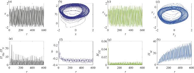
Figure 9. This figure illustrates the chaotic firing state of a memristor synapse-coupled system involving a neuron and a skeletal muscle cell: (a) the membrane potential of the neuron; (b) the attractor of the neuron circuit; (c) the membrane potential of the skeletal muscle cell; (d) the attractor of the skeletal muscle cell circuit; (e) the temporal evolution of the Hamiltonian energy ratio between the skeletal muscle cell and the neuron; (f) the temporal evolution of the displacement of the active beam; (g) the temporal evolution of the kinetic energy of the active beam; (h) the temporal evolution of the field energy in the memristor-coupled channel. The parameter values are set to γ = 3.2, η1 = 0.4. |
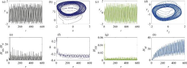
Figure 10. The chaotic firing state of a memristor synapse-coupled system involving a neuron and a skeletal muscle cell: (a) the membrane potential of the neuron; (b) the attractor of the neuron circuit; (c) the membrane potential of the skeletal muscle cell; (d) the attractor of the skeletal muscle cell circuit; (e) the temporal evolution of the Hamiltonian energy ratio between the skeletal muscle cell and the neuron; (f) the temporal evolution of the displacement of the active beam; (g) the temporal evolution of the kinetic energy of the active beam; (h) the temporal evolution of the field energy in the memristor-coupled channel. The parameter values are set to γ = 1.0, η1 = 2.0. |
When the parameter γ is set to 1, the membrane potential of the skeletal muscle cell exhibits periodic oscillations, as shown in figure 7(c). In contrast, when the parameter γ is increased to 3.2, the membrane potential of the skeletal muscle cell transitions to a chaotic state, as depicted in figure 9(c). According to figures 9(a) and (b), the membrane potential of the neuron also displays a chaotic state. The energy ratio between the skeletal muscle cell and the neuron, the displacement of the active beam, and the kinetic energy of the active beam all have large amplitudes initially, then rapidly decrease, and finally maintain chaotic oscillations within a certain range, as shown in figures 9(e), (f), and (g). The field energy in the coupled channel exhibits an increasing trend over time, as illustrated in figure 9(h).
In figure 7, when the parameter η1 is set to 0.4, the membrane potential of the skeletal muscle cell exhibits periodic oscillations, as shown in figure 7(c). In contrast, when the parameter η1 is increased to 2, the membrane potential of the skeletal muscle cell transitions to a chaotic state, as depicted in figure 10(c). According to figures 10(a) and (b), the neuron’s membrane potential also displays a chaotic state. The energy ratio between the skeletal muscle cell and the neuron, the displacement of the active beam, and the kinetic energy of the active beam all have large amplitudes initially, then rapidly decrease, and finally maintain chaotic oscillations within a certain range, as shown in figures 10(e), (f), and (g). The field energy in the coupled channel exhibits an increasing trend over time, as illustrated in figure 10(h). Furthermore, the Hamiltonian energy of the skeletal muscle cell also includes the magnetic field energy stored in the inductor of the circuit’s window structure, the elastic potential energy of the spring, and the kinetic energy of the active beam. These three parts of the energy are related to the values of the parameters k1 and m3. Bifurcation analysis and maximum Lyapunov index analysis were conducted on these two parameters, with the results shown in figure 11.
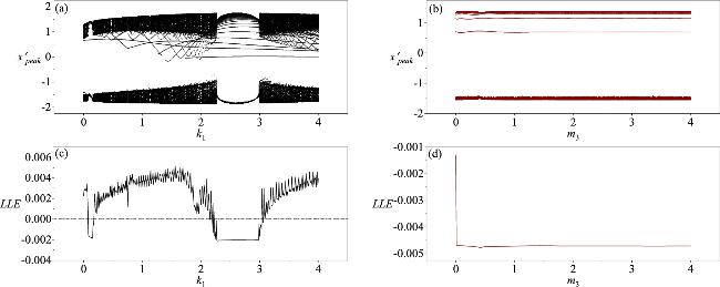
Figure 11. The bifurcation diagrams and Lyapunov exponents for the variable direction parameters k1 and m3 when a memristor synapse couples a neuron and a skeletal muscle cell. The parameters corresponding to the figures are: (a, c) m3 = 0.1; (b, d) k1 = 0.1; with a = 0.7, b = 0.3, c = 0.4, ξ = 0.175, I0 = 0.1, A = 0.4, λM = 0.1, α = 0.1, β = 0.1, γ = 3.2, η1 = 0.4, η2 = 0.12, k2 = 0.1, k3 = 0.1, m1 = 0.1, m2 = 0.1, ω = 1.3. The initial conditions of the system are (0.2, 0.1, 0, 0.1, 0.1, 0.1, 0.1, 0.1). |
It can be observed from figure 11 that altering the parameter k1, the oscillation pattern of the skeletal muscle cell membrane potential transitions from periodic to chaotic states or vice versa. However, changes in the parameter m3 do not cause transitions in the state of the skeletal muscle cell membrane potential. Under the conditions shown in figures 11(b), (d), the system remains in a periodic state, as depicted in figure 7. To further confirm the impact of changing the parameter k1 on the coupled system, figure 12 was calculated, with the parameters set to a = 0.7, b = 0.3, c = 0.4, ξ = 0.175, I0 = 0.1, A = 0.4, λM = 0.1, α = 0.1, β = 0.1, γ = 3.2, η1 = 0.4, η2 = 0.12, k1 = 1.8, k2 = 0.1, k3 = 0.1, m1 = 0.1, m2 = 0.1, m3 = 0.1, ω = 1.3, m4 = 1, m5 = 0.1. The initial values are (0.2, 0.1, 0, 0.1, 0.1, 0.1, 0.1, 0.1).
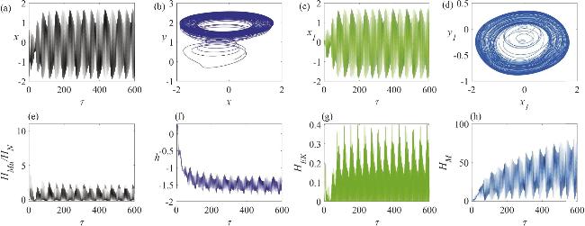
Figure 12. The chaotic firing state of a memristor synapse-coupled system involving a neuron and a skeletal muscle cell: (a) the membrane potential of the neuron; (b) the attractor of the neuron circuit; (c) the membrane potential of the skeletal muscle cell; (d) the attractor of the skeletal muscle cell circuit; (e) the temporal evolution of the Hamiltonian energy ratio between the skeletal muscle cell and the neuron; (f) the temporal evolution of the displacement of the active beam; (g) the temporal evolution of the kinetic energy of the active beam; (h) the temporal evolution of the field energy in the memristor-coupled channel. The parameter values are set to k1 = 1.8. |
When the parameter k1 is set to 0.1, the membrane potential of the skeletal muscle cell exhibits periodic oscillations, as shown in figure 7(c). Conversely, when the parameter k1 is increased to 1.8, the membrane potential of the skeletal muscle cell transitions to a chaotic state, as depicted in figure 12(c). Observations from figures 12(a) and (b) indicate that the neuron’s membrane potential also displays a chaotic state. The energy ratio between the skeletal muscle cell and the neuron, as well as the displacement of the active beam, initially have large amplitudes, then rapidly decrease, and ultimately maintain chaotic oscillations within a certain range, as illustrated in figures 12(e) and (f). The kinetic energy of the active beam maintains chaotic oscillations within the range of 0 to 0.4, as shown in figure 12(g). The field energy in the coupled channel exhibits an increasing trend over time, as demonstrated in figure 12(h). In practice, the synaptic coupling between neurons and skeletal muscle cells is regulated by the energy relationship between the two cells. Thus, the establishment of the coupling channel is influenced by the combined energy of the skeletal muscle cell and the neuron. Here, the ratio of the skeletal muscle cell’s energy to the neuron’s energy is set to control the memristive synapse between the two cells. When the ratio of energy between the two cells exceeds the threshold (ϵ = 25), the synapse between the two cells begins to form, and the coupling strength of the coupling channel increases exponentially over time. When the energy ratio between the two cells falls below the threshold, the coupling strength ceases to grow, and the coupling channel stabilizes. Under the aforementioned conditions, by expressing the coupling strength in equation (5 ) with equation (12 ), the evolution of the memristive synapse coupling strength, the energy ratio between the skeletal muscle cell and the neuron, and the field energy in the coupling channel over time were calculated, with the results shown in figure 13.
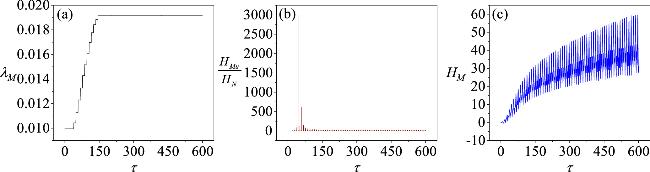
Figure 13. The evolution of coupling strength, the energy ratio between skeletal muscle cells and neurons, and the field energy in the coupling channel over time when the coupling strength is adaptively regulated. The parameters are selected as: a = 0.7, b = 0.3, c = 0.4, ξ = 0.175, I0 = 0.1, A = 0.4, α = 0.1, β = 0.1, γ = 1, η1 = 0.4, η2 = 0.12, k1 = 0.1, k2 = 0.1, k3 = 0.1, m1 = 0.1, m2 = 0.1, m3 = 0.1, m4 = 1, m5 = 0.1, σ = 0.1, ϵ = 25. The initial conditions are (0.2, 0.1, 0, 0.1, 0.1, 0.1, 0.1, 0.1). The initial value of the coupling strength λM(0) is 0.01. |
As depicted in figure 13, when memristive synapses couple skeletal muscle cells and neuron cells, and the coupling strength of the memristive synapses is regulated by the energy ratio between the two cells, the coupling strength continuously increases when the energy ratio exceeds the threshold (ϵ = 25). This leads to a continuous enhancement of information transfer and energy exchange between the two cells. Conversely, when the energy ratio falls below the threshold, the coupling strength of the synapses between the two cells ceases to increase, stabilizing the coupling channel, as shown in figure 13(a). The evolution of the energy ratio between the two neurons over time is illustrated in figure 13(b), corroborating the results presented in figure 13(a). As coupling progresses, the field energy stored in the coupling channel continually accumulates, with the amplitude of the field energy in the channel increasing, as depicted in figure 13(c).
4. Conclusion
The study begins with an in-depth analysis of the dynamic characteristics of a single neuron circuit. By adjusting the angular frequency of the external signal stimulation voltage, it was observed that the neuron’s membrane potential exhibited various firing modes such as clustered firing, spiking firing, and chaotic firing under different stimulation conditions. Subsequently, neurons with different firing modes were coupled with skeletal muscle cells via memristive synapses. The results post-coupling indicated significant changes in the firing modes of the neurons. Additionally, neurons with different firing modes also induced oscillations in the membrane potential of the skeletal muscle cells after coupling, primarily manifesting as periodic and chaotic patterns. The displacement of the active beam over time also exhibited oscillations that corresponded to the state of the coupled neuron, with periodic oscillations observed for clustered and chaotic firing neurons coupled with skeletal muscle cells, and chaotic oscillations for spiking firing neurons coupled with skeletal muscle cells. Furthermore, this study conducted bifurcation analysis and Lyapunov exponent analysis on parameters within the Hamiltonian energy of skeletal muscle cells. It was found that adjusting the capacitor parameter γ and the inductor parameter η1, which simulate the membrane potential of skeletal muscle cells, could alter the firing modes of neurons and skeletal muscle cells. Similarly, changes in the inductor parameter k1 within the mechanical structure could also trigger transitions of the neuron’s membrane potential from chaotic states to periodic states or vice versa. However, changes in the parameter m3, which is related to the kinetic energy of the moving arm and the elastic potential energy of the spring in the mechanical structure, do not cause transitions in the oscillation patterns of the membrane potentials of neurons and skeletal muscle cells. Ultimately, by using the energy ratio between neuron cells and skeletal muscle cells, the coupling strength of the coupling channel was adaptively regulated using a step function, achieving adaptive growth of the coupling strength to a specific threshold. This optimization enhanced the interaction between neurons and skeletal muscle cells. This finding provides a new perspective for understanding the complex interactions between neurons and muscle cells and lays an important theoretical foundation for future research in related fields.