


1. Introduction
Toda lattice equation, initially formulated by Toda in 1967, is a fundamental model within the realm of mathematical physics, which describes the dynamics of a one-dimensional lattice of particles with exponential interactions between nearest neighbors [1, 2]. Initially formulated to investigate wave propagation in one-dimensional nonlinear lattices, the Toda lattice equation has found widespread applications in various fields including condensed matter physics, biophysics and optical systems [3] outside its original physical context. Moreover, some generalized Toda lattice equation and modified Toda lattice equation have also been proposed and discussed [4, 5]. In this study, we delve deeper into the analysis of the following generalized Toda lattice equation with four potentials [4]: 2 ) with respect to n and t, The translation operator E is is characterized by its action Ef(n, t) = f(n + 1, t) = fn+1, the symbol λ denotes a spectral parameter that has nothing to do with t, and subscript t denote partial derivatives with respect to t. Setting cn = dn = 0, equation (1 ) degenerates into the celebrated Toda lattice equation [2, 3]. Since Geng et al proposed equation (1 ) in 2006, equation(1 ) has garnered considerable attention. In [4], the integrable hierarchy and Hamiltonian structure of equation (1 ) have been formulated. In [6], explicit quasi-periodic solutions were constructed. Furthermore, reference [7] provided the infinite number of conservation laws for equation (1 ) and constructed the N-fold DT in matrix form to obtain solitary wave solutions. So far, the continuum limit, generalization Darboux transformation (DT), and singular rational and mixed solutions of equation (1 ) have not been studied. Therefore, the motivation of this paper is to investigate the continuous limit and singular rational solution structures.
$\begin{eqnarray}\left\{\begin{array}{l}{a}_{n,t}={a}_{n}({c}_{n+1}{d}_{n+1}-{c}_{n}{d}_{n}+{b}_{n}-{b}_{n+1}),\\ {b}_{n,t}={a}_{n-1}-{a}_{n},\\ {c}_{n,t}=-{a}_{n-1}{c}_{n-1},\\ {d}_{n,t}={d}_{n+1}{a}_{n},\end{array}\right.\end{eqnarray}$
which possesses a 3 × 3 matrix Lax pair, where an, bn, cn, dn are four potential functions about n, t, and its 3 × 3 matrix Lax pair admits $\begin{eqnarray}\begin{array}{l}E{\phi }_{n}={L}_{n}{\phi }_{n}=\left(\begin{array}{ccc}\lambda +{b}_{n} & {c}_{n} & -1\\ {d}_{n} & 1 & 0\\ {a}_{n} & 0 & 0\end{array}\right){\phi }_{n},\quad {\phi }_{n,t}={V}_{n}{\phi }_{n}\\ \quad =\,\left(\begin{array}{ccc}0 & 0 & -1\\ 0 & 0 & {d}_{n}\\ {a}_{n-1} & -{a}_{n-1}{c}_{n-1} & {c}_{n}{d}_{n}-(\lambda +{b}_{n})\end{array}\right){\phi }_{n},\end{array}\end{eqnarray}$
where ${\phi }_{n}={({\varphi }_{n},{\psi }_{n},{\chi }_{n})}^{T}$ represents the characteristic function of equation (Analyzing exact solutions of discrete nonlinear lattice equations is essential for interpreting physical phenomena such as wave propagation in fluid dynamics, plasmas, and elastic media [3, 8, 9]. Various powerful methods have been employed to derive these solutions, including the Jacobi elliptic function expansion [10], Hirota bilinear approaches [11], Bäcklund transformation [12], the inverse scattering transformation [13, 14], Riemann–Hilbert method [15], the Lie symmetry method [16, 17], $({G}^{{\prime} }/G)$-expansion method [18], and the DT [5, 7, 19–25]. The DT method is particularly effective for solving discrete nonlinear lattice equations linked to 2 × 2 matrix spectral problems [5, 19, 20] and 3 × 3 matrix spectral problems [7, 21–25], and its generalized form further enhances its capability to generate a wider range of solutions. The generalized (m, 3N − m)-fold DT is an extension of the usual DT that has been successfully applied to systems such as Blaszak–Marciniak lattice and Belov–Chaltikian lattice equations, which are connected to 3 × 3 matrix spectral problems [24, 25]. Nevertheless, equation (1 ) has not been investigated using this method, particularly with respect to its singular rational solutions and singular mixed rational-exponential solutions.
The subsequent sections of this article are structured as follows. Section 2 focuses on mapping the discrete four-potential Toda lattice equation to two continuous counterparts. In section 3 , the discrete generalized (m, 3N − m)-fold DT for equation (1 ) is formulated based on the established Lax pair (2 ). Section 4 employs the generalized DT to derive rational and mixed rational-exponential solutions, which are analyzed and depicted graphically. The final section provides a summary of the key results.
2. Continuous limit
(i) Using the continuous condition 1 ) admits a continuous nonlinear counterpart as follows:
$\begin{eqnarray*}\left\{\begin{array}{rc}{a}_{n} & =\epsilon q(\epsilon n+\epsilon t,\epsilon t)=\epsilon q(x,\tau ),\\ {b}_{n} & =\epsilon p(\epsilon n+\epsilon t,\epsilon t)=\epsilon p(x,\tau ),\\ {c}_{n} & =\epsilon r(\epsilon n+\epsilon t,\epsilon t)=\epsilon r(x,\tau ),\\ {d}_{n} & =\epsilon s(\epsilon n+\epsilon t,\epsilon t)=\epsilon s(x,\tau ),\end{array}\right.\end{eqnarray*}$
in which ε is an extremely small parameter. equation ( $\begin{eqnarray}\left\{\begin{array}{l}({q}_{\tau }+{q}_{x})\epsilon +O({\epsilon }^{2})=0,\\ ({p}_{\tau }+{p}_{x}+{q}_{x})\epsilon +O({\epsilon }^{2})=0,\\ ({r}_{\tau }+{r}_{x}+rq)\epsilon +O({\epsilon }^{2})=0,\\ ({s}_{\tau }+{s}_{x}-sq)\epsilon +O({\epsilon }^{2})=0,\end{array}\right.\end{eqnarray}$
as O(ε2) is neglected.(ii) In addition, by means of a following different continuous condition: 1 ) can be matched to new continuous nonlinear equation as below
$\begin{eqnarray*}\left\{\begin{array}{l}{a}_{n}=\epsilon q(\epsilon n+\epsilon t,\epsilon t)=\epsilon q(x,\tau ),\\ {b}_{n}=\epsilon p(\epsilon n+\epsilon t,\epsilon t)=\epsilon p(x,\tau ),\\ {c}_{n}=\epsilon r(\epsilon n+\epsilon t,\epsilon t)+1=\epsilon r(x,\tau )+1,\\ {d}_{n}=\epsilon s(\epsilon n+\epsilon t,\epsilon t)+1=\epsilon s(x,\tau )+1.\end{array}\right.\end{eqnarray*}$
Equation ( $\begin{eqnarray}\left\{\begin{array}{l}{q}_{\tau }+{q}_{x}-{r}_{x}(q+sq)-{s}_{x}(q+rq)=0,\\ {p}_{\tau }+{p}_{x}+{q}_{x}=0,\\ {r}_{\tau }+{r}_{x}+r+rq=0,\\ {s}_{\tau }+{s}_{x}-s-sq=0.\end{array}\right.\end{eqnarray}$
3. Discrete DT
This section focuses on developing the discrete generalized (m, 3N − m)-fold DT for equation (1 ) using its associated Lax pair equation (2 ). To accomplish this, we proceed by considering the transformation: 2 ) and (5 ), we derive the relationships:
$\begin{eqnarray}{\widetilde{\phi }}_{n}={T}_{n}{\phi }_{n},\end{eqnarray}$
with ${\widetilde{\phi }}_{n}$ mandated to meet ${\widetilde{\phi }}_{n+1}={\widetilde{U}}_{n}{\widetilde{\phi }}_{n},$ and ${\widetilde{\phi }}_{n,t}={\widetilde{V}}_{n}\widetilde{{\phi }_{n}}$. From equations ( $\begin{eqnarray}{\widetilde{U}}_{n}={T}_{n+1}{U}_{n}{T}_{n}^{-1},\quad {\widetilde{V}}_{n}=({T}_{n,t}+{T}_{n}{V}_{n}){T}_{n}^{-1},\end{eqnarray}$
where ${\widetilde{U}}_{n},{\widetilde{V}}_{n}$ and Un, Vn share identical matrix structures, differing only in the substitution of an, bn, cn, dn with ${\widetilde{a}}_{n},{\widetilde{b}}_{n},{\widetilde{c}}_{n},{\widetilde{d}}_{n}$. This framework allows us to construct a specific DT matrix as: $\begin{eqnarray}{T}_{n}(\lambda )=\left(\begin{array}{ccc}{\lambda }^{N}+\displaystyle \sum _{j=0}^{N-1}{D}_{n}^{(j)}{\lambda }^{j}\qquad \quad & \displaystyle \sum _{j=0}^{N-1}{E}_{n}^{(j)}{\lambda }^{j}\qquad \quad & \displaystyle \sum _{j=0}^{N-1}{F}_{n}^{(j)}{\lambda }^{j}\\ \displaystyle \sum _{j=0}^{N-1}{G}_{n}^{(j)}{\lambda }^{j}\qquad \quad & {\lambda }^{N}+\displaystyle \sum _{j=0}^{N-1}{H}_{n}^{(j)}{\lambda }^{j}\qquad \quad & \displaystyle \sum _{j=0}^{N-1}{J}_{n}^{(j)}{\lambda }^{j}\\ \displaystyle \sum _{j=0}^{N-1}{K}_{n}^{(j)}{\lambda }^{j}\qquad \quad & \displaystyle \sum _{j=0}^{N-1}{W}_{n}^{(j)}{\lambda }^{j}\qquad \quad & (1+{F}_{n}^{(N-1)}){\lambda }^{N}+\displaystyle \sum _{j=0}^{N-1}{R}_{n}^{(j)}{\lambda }^{j}\end{array}\right),\end{eqnarray}$
where N presents the order of DT, and ${D}_{n}^{(j)}\ {E}_{n}^{(j)}\ {F}_{n}^{(j)}\ {G}_{n}^{(j)}\ {H}_{n}^{(j)}\ {J}_{n}^{(j)}\ {K}_{n}^{(j)}\ {W}_{n}^{(j)}\ {R}_{n}^{(j)}$ are unknown functions, which will be derived from following linear system: $\displaystyle \sum _{j=0}^{{k}_{i}}{T}_{n}^{(j)}({\lambda }_{i}){\phi }_{n}^{({k}_{i}-j)}({\lambda }_{i})=0\,\ (3N=m+\displaystyle \sum _{i=1}^{m}{k}_{i},\ i=1,2,\cdots \,,m)$, where ${\phi }_{n}^{(k)}({\lambda }_{i})=\frac{1}{k!}\frac{{\partial }^{k}}{\partial {\lambda }_{i}^{k}}{\phi }_{n}({\lambda }_{i})$ is the term of Taylor expansion ${\phi }_{i,n}({\lambda }_{i}+\varepsilon )={\sum }_{k=0}^{\infty }{\phi }_{i,n}^{(k)}{\varepsilon }^{k}$, and ${T}_{n}^{(j)}$ is provided by binomial expansion of $T({\lambda }_{i}+\varepsilon )={T}_{n}^{(0)}+{T}_{n}^{(1)}\varepsilon +{T}_{n}^{(2)}{\varepsilon }^{2}+\cdots +{T}_{n}^{({k}_{i})}{\varepsilon }^{{k}_{i}}$.For the derivation of explicit rational and mixed solutions of equation (1 ), the discrete DT reported in [7, 21] must be extended to the generalized DT. Based on equations (6 ) and (7 ),the relationships between the new and old potential functions are formulated as:
$\begin{eqnarray}\begin{array}{rcl}{\widetilde{a}}_{n} & = & {K}_{n+1}^{(N-1)}+(1+{F}_{n+1}^{(N-1)}){a}_{n},\,\,{\widetilde{b}}_{n}={D}_{n+1}^{(N-1)}+{b}_{n}-{D}_{n}^{(N-1)},\\ {\widetilde{c}}_{n} & = & {c}_{n}-{E}_{n}^{(N-1)},\qquad \qquad \qquad {\widetilde{d}}_{n}={G}_{n+1}^{(N-1)}+{d}_{n},\end{array}\end{eqnarray}$
where ${D}_{n}^{(N-1)}$, ${E}_{n}^{(N-1)}$, ${F}_{n}^{(N-1)}$, ${G}_{n}^{(N-1)}$, ${K}_{n}^{(N-1)}$ are defined as: ${D}_{n}^{(N-1)}=\frac{{\rm{\Delta }}{D}_{n}^{(N-1)}}{{{\rm{\Delta }}}_{N}}$, ${E}_{n}^{(N-1)}=\frac{{\rm{\Delta }}{E}_{n}^{(N-1)}}{{{\rm{\Delta }}}_{N}}$, ${F}_{n}^{(N-1)}=\frac{{\rm{\Delta }}{F}_{n}^{(N-1)}}{{{\rm{\Delta }}}_{N}}$, ${G}_{n}^{(N-1)}=\frac{{\rm{\Delta }}{G}_{n}^{(N-1)}}{{{\rm{\Delta }}}_{N}}$, ${K}_{n}^{(N-1)}=\frac{{\rm{\Delta }}{K}_{n}^{(N-1)}}{{{\rm{\Delta }}}_{N}}$, and ${{\rm{\Delta }}}_{N}=\det ({[\underset{N}{\overset{(1)}{{\rm{\Delta }}}},{{\rm{\Delta }}}_{N}^{(2)},\ldots ,{{\rm{\Delta }}}_{N}^{(m)}]}^{T})$, in which ${{\rm{\Delta }}}_{N}=\det ({[\underset{N}{\overset{(1)}{{\rm{\Delta }}}},{{\rm{\Delta }}}_{N}^{(2)},\ldots ,{{\rm{\Delta }}}_{N}^{(m)}]}^{T})$ with ${{\rm{\Delta }}}_{N}^{(i)}={({{\rm{\Delta }}}_{N,j,r}^{(i)})}_{({k}_{i}+1)\times 3N}$ is derived through the following expressions: $\begin{eqnarray*}{{\rm{\Delta }}}_{N,j,r}^{(i)}=\left\{\begin{array}{l}\displaystyle \sum _{k=0}^{j-1}{C}_{N-r}^{k}{\lambda }_{i}^{N-r-k}{\varphi }_{i,n}^{(j-1-k)},\,\,\,as\,\,\,1\leqslant j\leqslant {k}_{i}+1,\,1\leqslant r\leqslant N,\\ \displaystyle \sum _{k=0}^{j-1}{C}_{2N-r}^{k}{\lambda }_{i}^{2N-r-k}{\psi }_{i,n}^{(j-1-k)},\,\,\,as\,\,\,1\leqslant j\leqslant {k}_{i}+1,\,N+1\leqslant r\leqslant 2N,\\ \displaystyle \sum _{k=0}^{j-1}{C}_{3N-r}^{k}{\lambda }_{i}^{3N-r-k}{\chi }_{i,n}^{(j-1-k)},\,\,\,as\,\,\,1\leqslant j\leqslant {k}_{i}+1,\,2N+1\leqslant r\leqslant 3N.\\ \end{array}\right.\end{eqnarray*}$
Here, ${\rm{\Delta }}{D}_{n}^{(N-1)},\ {\rm{\Delta }}{E}_{n}^{(n)},\ {\rm{\Delta }}{F}_{n}^{(N-1)}$ arise from transforming the determinant ΔN by substituting its first, (N + 1)th and (2N + 1)th columns of with ${({\omega }^{(1)},{\omega }^{(2)},\ldots ,{\omega }^{(m)})}^{T}$, in that order, where ${\omega }^{(i)}={({\omega }_{j}^{(i)})}_{({k}_{i}+1)\times 1}$ and ${\omega }_{j}^{(i)}=-{\sum }_{k=0}^{j-1}{C}_{N}^{k}{\lambda }_{i}^{N-k}{\varphi }_{i,n}^{(j-1-k)}$. Similarly, ${\rm{\Delta }}{G}_{n}^{(N-1)}$ is derived by exchanging the first column of ΔN with ${({\mu }^{(1)},{\mu }^{(2)},\ldots ,{\mu }^{(m)})}^{T}$, where ${\mu }^{(i)}={({\mu }_{j}^{(i)})}_{({k}_{i}+1)\times 1}$, in which ${\mu }_{j}^{(i)}=-{\sum }_{k=0}^{j-1}{C}_{N}^{k}{\lambda }_{i}^{N-k}{\psi }_{i,n}^{(j-1-k)}$. ${\rm{\Delta }}{K}_{n}^{(N-1)}$ can be generated by replacing the first column of the determinant ΔN with ${({\beta }^{(1)},{\beta }^{(2)},\ldots ,{\beta }^{(m)})}^{T}$, where ${\beta }^{(i)}={({\beta }_{j}^{(i)})}_{({k}_{i}+1)\times 1}$ and ${\beta }_{j}^{(i)}=-(1+{c}_{n}^{(N-1)})\displaystyle \sum _{k=0}^{j-1}{C}_{N}^{k}{\lambda }_{i}^{N-k}{\chi }_{i,n}^{(j-1-k)}$.4. Explicit exact solutions
Solitons are travelling waves that remain structurally stable and invariant for long periods of time during propagation, and have very important roles in nonlinear optics, electromagnetism, Bose–Einstein condensation, plasma, and other fields [26, 27]. In this section, we will consider some new singular rational soliton and mixed rational-exponential structures of equation (1 ) by using the DT.
The fundamental solution can be readily obtained by substituting the seed solutions an = bn = 1, cn = dn = 0 into equation (2 ), yielding 9 ), but we will not make Taylor expansion at λk (k ≠ 1).
$\begin{eqnarray}\begin{array}{l}{\phi }_{n}({\lambda }_{k})=\left(\begin{array}{l}{\varphi }_{n}\\ {\psi }_{n}\\ {\chi }_{n}\end{array}\right)\\ \quad =\left(\begin{array}{l}{C}_{1,k}{\tau }_{1}^{n}{{\rm{e}}}^{-\tfrac{t}{{\tau }_{1}}+{\rm{\Theta }}}+{C}_{2,k}{\tau }_{2}^{n}{{\rm{e}}}^{-\tfrac{t}{{\tau }_{2}}+{\rm{\Theta }}}+{C}_{3,k}{\tau }_{3}^{n}{{\rm{e}}}^{-\tfrac{t}{{\tau }_{3}}-{\rm{\Theta }}}\\ {C}_{1,k}+{C}_{2,k}+{C}_{3,k}\\ {C}_{1,k}{\tau }_{1}^{n-1}{{\rm{e}}}^{-\tfrac{t}{{\tau }_{1}}+{\rm{\Theta }}}+{C}_{2,k}{\tau }_{2}^{n-1}{{\rm{e}}}^{-\tfrac{t}{{\tau }_{2}}+{\rm{\Theta }}}+{C}_{3,k}{\tau }_{3}^{n-1}{{\rm{e}}}^{-\tfrac{t}{{\tau }_{3}}-{\rm{\Theta }}}\end{array}\right),\end{array}\end{eqnarray}$
in which ${\rm{\Theta }}=\sqrt{{\lambda }^{2}+2\lambda -3}{\sum }_{j=0}^{n=3N-1}{\varkappa }_{j}{\epsilon }^{j}$, and C1,k, C2,k, C3,k are arbitrary constants. Meanwhile, τk (k = 1, 2, 3) serve as the solutions to the cubic equation τ3 − (λ + 2)τ2 + (λ + 2)τ − 1 = 0. If λ = λ1 = 1, we make two types of Taylor expansions of equation (• Type 1 Given the parameters C1,1 = 0 and C2,1 = C3,1 = 1 and λ = λ1 + ε2, we list the first three terms of Taylor expansion of equation (9 ) as
$\begin{eqnarray*}\begin{array}{rcl}{\phi }_{n}^{(0)} & = & \left(\begin{array}{l}{\varphi }_{n}^{(0)}\\ {\psi }_{n}^{(0)}\\ {\mathrm{* \chi }}_{n}^{(0)}\end{array}\right)=2\left(\begin{array}{l}{{\rm{e}}}^{-t}\\ 1\\ {{\rm{e}}}^{-t}\end{array}\right),\\ {\phi }_{n}^{(1)} & = & \left(\begin{array}{l}{\varphi }_{n}^{(1)}\\ {\psi }_{n}^{(1)}\\ {\chi }_{n}^{(1)}\end{array}\right)={{\rm{e}}}^{-t}\left(\begin{array}{l}{\alpha }^{2}-t\\ 0\\ {\alpha }^{2}-2\alpha -t+1\end{array}\right),\end{array}\end{eqnarray*}$
$\begin{eqnarray*}\begin{array}{l}{\phi }_{n}^{(2)}=\left(\begin{array}{l}{\varphi }_{n}^{(2)}\\ {\psi }_{n}^{(2)}\\ {\chi }_{n}^{(2)}\end{array}\right)\\ \quad =\,{{\rm{e}}}^{-t}\left(\begin{array}{l}{\alpha }^{4}-(6t-6){\alpha }^{2}-10n\alpha +3{n}^{2}\\ 0\\ {\alpha }^{4}-4{\alpha }^{3}-(6t-5){\alpha }^{2}+16t\alpha -2\alpha +3{t}^{2}-10t\end{array}\right),\end{array}\end{eqnarray*}$
in which α = n + t.• Type 2 When ${C}_{1,1}=0,{C}_{2,1}=-\frac{1}{\epsilon },{C}_{3,1}=\frac{1}{\epsilon }$ and λ = λ1 + ε2 are specified, we only list the first three of Taylor expansion as:
$\begin{eqnarray*}\begin{array}{rcl}{\phi }_{n}^{(0)} & = & \left(\begin{array}{l}{\varphi }_{n}^{(0)}\\ {\psi }_{n}^{(0)}\\ {\chi }_{n}^{(0)}\end{array}\right)\,=\,2{{\rm{e}}}^{-t}\left(\begin{array}{l}\alpha \\ 0\\ \alpha -1\end{array}\right),\,{\phi }_{n}^{(1)}=\left(\begin{array}{l}{\varphi }_{n}^{(1)}\\ {\psi }_{n}^{(1)}\\ {\chi }_{n}^{(1)}\end{array}\right)=-\displaystyle \frac{{{\rm{e}}}^{-t}}{12}\left(\begin{array}{l}4{\alpha }^{3}-(12t+1)\alpha +4t\\ 0\\ 4{\alpha }^{3}-12{\alpha }^{2}-(12t-27)\alpha -16n-3\end{array}\right),\\ {\phi }_{n}^{(2)} & = & \left(\begin{array}{l}{\varphi }_{n}^{(2)}\\ {\psi }_{n}^{(2)}\\ {\chi }_{n}^{(2)}\end{array}\right)\\ & = & -\displaystyle \frac{{{\rm{e}}}^{-t}}{640}\left(\begin{array}{l}16{\alpha }^{5}-160{\alpha }^{4}+(160n+360){\alpha }^{3}-(640n+120){\alpha }^{2}+240{n}^{2}\alpha +(280n-15)\alpha -160{n}^{2}+24n\\ 0\\ 16{\alpha }^{5}-240{\alpha }^{4}+160n{\alpha }^{3}+1000{\alpha }^{3}-(1120n+1200){\alpha }^{2}+(240{n}^{2}+1560n+225)\alpha -400{n}^{2}-256n+15\end{array}\right).\end{array}\end{eqnarray*}$
4.1. First-order exact solutions
In this part, we will focus on the first-order exact solutions when m = 3, N = 1.
Case (i). Exact exponential function solution or hyperbolic function solution
Employing the (3, 0)-fold DT as m = 3 and N = 1, specifically, for λ1, we employ the first term of Type 1 Taylor expansion with coefficients C1,1 = 0 and C2,1 = C3,1 = 1, excluding rational polynomial terms. Additionally, for ${\lambda }_{2}=\frac{3}{2}$ and ${\lambda }_{3}=\frac{13}{4}$, we refrain from expanding and instead assign coefficients C1,2 = C2,2 = 0, C3,2 = 1 and C1,3 = C2,3 = 0, C3,3 = 1 respectively. Subsequently, based on equation (8 ), we derive the first-order exponential function solution as detailed below:
$\begin{eqnarray}{\tilde{a}}_{n}=1-\displaystyle \frac{21{\Gamma }_{3}}{8{\Gamma }_{1}^{2}},\quad {\tilde{b}}_{n}=1+\displaystyle \frac{21{\Gamma }_{4}}{4{\Gamma }_{1}{\Gamma }_{2}},\quad {\tilde{c}}_{n}=-\displaystyle \frac{21}{4{\Gamma }_{2}}{{\rm{e}}}^{2n\mathrm{ln}2-\tfrac{3t}{2}},\quad {\tilde{d}}_{n}=-\displaystyle \frac{{{\rm{e}}}^{t}{\Gamma }_{5}}{2{\Gamma }_{1}},\end{eqnarray}$
where
$\begin{eqnarray*}\begin{array}{rcl}{\Gamma }_{1} & = & 6{{\rm{e}}}^{\tfrac{5n}{2}\mathrm{ln}2}\sinh \left(\displaystyle \frac{n}{2}\mathrm{ln}2+\displaystyle \frac{t}{2}\right)-{{\rm{e}}}^{n\mathrm{ln}2-\tfrac{7t}{8}}\sinh \left(n\mathrm{ln}2+\displaystyle \frac{3t}{8}\right),\\ {\Gamma }_{2} & = & -3{{\rm{e}}}^{\tfrac{5n}{2}\mathrm{ln}2}\sinh \left(\displaystyle \frac{n}{2}\mathrm{ln}2+\displaystyle \frac{t}{2}\right)+4{{\rm{e}}}^{n\mathrm{ln}2-\tfrac{7t}{8}}\sinh \left(n\mathrm{ln}2+\displaystyle \frac{3t}{8}\right),\\ {\Gamma }_{3} & = & -3{{\rm{e}}}^{\tfrac{5n}{2}\mathrm{ln}2-\tfrac{5t}{4}}\sinh \left(\displaystyle \frac{n}{2}\mathrm{ln}2+\displaystyle \frac{t}{2}\right)+4{{\rm{e}}}^{4n\mathrm{ln}2-\tfrac{3t}{8}}\sinh \left(n\mathrm{ln}2+\displaystyle \frac{3t}{8}\right),\\ {\Gamma }_{4} & = & 6{{\rm{e}}}^{\tfrac{5n}{2}\mathrm{ln}2-\tfrac{5t}{4}}\sinh \left(\displaystyle \frac{n}{2}\mathrm{ln}2+\displaystyle \frac{t}{2}\right)-{{\rm{e}}}^{4n\mathrm{ln}2-\tfrac{3t}{8}}\sinh \left(n\mathrm{ln}2+\displaystyle \frac{3t}{8}\right),\\ {\Gamma }_{5} & = & 2{{\rm{e}}}^{\tfrac{3n}{2}\mathrm{ln}2-\tfrac{3t}{8}}\sinh \left(\displaystyle \frac{3n}{2}\mathrm{ln}2+\displaystyle \frac{7t}{8}\right)+7{{\rm{e}}}^{n\mathrm{ln}2-\tfrac{3t}{4}}\sinh \left(\displaystyle \frac{n}{2}\mathrm{ln}2+\displaystyle \frac{t}{2}\right),\end{array}\end{eqnarray*}$
from which we can derive that ${\widetilde{a}}_{n},\ {\widetilde{d}}_{n}$ share an identical singular trajectory curve, denoted as Γ1 = 0, whereas ${\widetilde{c}}_{n}$ possesses a distinct singular trajectory curve, labeled as Γ2 = 0, ${\widetilde{b}}_{n}$ owns two different singularity trajectory curves Γ1 = 0, Γ2 = 0. At the same time, the three-dimensional structures of solution ${\widetilde{a}}_{n},\ {\widetilde{b}}_{n},\ {\widetilde{c}}_{n},\ {\widetilde{d}}_{n}$ are displayed in figures 1(a1)–(a4) respectively, while the associated singular trajectory plots corresponding to ${\widetilde{a}}_{n},\ {\widetilde{b}}_{n},\ {\widetilde{c}}_{n},\ {\widetilde{d}}_{n}$ are exhibited in figures 1(b1)–(b4).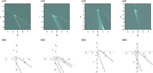
Figure 1. The structures of solution equation ( |
Case (ii). First-order mixed rational-exponential solution
Next, we perform the Taylor expansion of Type 2 at ε = 0 for λ1, and do the same arrangement with Case (i) for λ2, λ3, thereby deriving the first-order mixed rational-exponential solution as outlined below: 11 ) are displayed in figures 2(a1)–(a4) respectively. From solution equation (11 ), we can clearly know that ${\widetilde{a}}_{n},\ {\widetilde{d}}_{n}$ exist the same singularity trajectory curve: A1 = 0, ${\widetilde{b}}_{n}$ owns two singularity trajectory curves: A1 = 0, A2 = 0 while ${\widetilde{c}}_{n}$ haves one singularity trajectory curve: A2 = 0. figures 2(b1)–(b4) depict the singularity trajectory curves of ${\widetilde{a}}_{n},\ {\widetilde{b}}_{n},\ {\widetilde{c}}_{n}\ {\widetilde{d}}_{n}$, respectively.
$\begin{eqnarray}\left\{\begin{array}{l}{\tilde{a}}_{n}=1+\displaystyle \frac{{A}_{3}}{128{({A}_{1})}^{3}},\\ {\tilde{b}}_{n}=1+\displaystyle \frac{24\sqrt{2}\cosh (2{\xi }_{1}+\tfrac{1}{2}\mathrm{ln}\tfrac{9}{2})-49(3{\alpha }^{2}+2\alpha )-44}{16{A}_{1}{A}_{2}},\\ {\tilde{c}}_{n}=\displaystyle \frac{7(3\alpha +2){{\rm{e}}}^{\tfrac{n}{2}\mathrm{ln}2-\tfrac{9t}{8}}}{8{A}_{2}},\\ {\tilde{d}}_{n}=-\displaystyle \frac{7\alpha {{\rm{e}}}^{-\tfrac{n}{2}\mathrm{ln}2+\tfrac{9t}{8}}}{4{A}_{1}},\end{array}\right.\end{eqnarray}$
where $\begin{eqnarray*}\begin{array}{rcl}{A}_{1} & = & \sqrt{6}\alpha \cosh \left({\xi }_{1}+\frac{1}{2}\mathrm{ln}6\right)-2\sinh {\xi }_{1},\\ {A}_{2} & = & \sqrt{3}\alpha \cosh \left({\xi }_{1}+\frac{1}{2}\mathrm{ln}\frac{3}{4}\right)-2\sinh {\xi }_{1},\\ {A}_{3} & = & 1176\sqrt{6}{\alpha }^{3}\cosh \left({\xi }_{1}+\frac{1}{2}\mathrm{ln}6\right)+784\sqrt{66}{\alpha }^{2}\cosh .\\ & & \times \,\left({\xi }_{1}+\frac{1}{2}\mathrm{ln}\frac{24}{11}\right)+16\sqrt{38989}\alpha \cosh ({\xi }_{1}+\frac{1}{2}\mathrm{ln}\frac{127}{307})\\ & & -39\sqrt{2774}\sinh ({\xi }_{1}+\frac{1}{2}\mathrm{ln}\frac{73}{38}).\\ & & -192\sqrt{6}\alpha \cosh \left(3{\xi }_{1}+\frac{1}{2}\mathrm{ln}216\right)+384\sinh (3{\xi }_{1}+\mathrm{ln}6),\end{array}\end{eqnarray*}$
in which ${\xi }_{1}=\frac{3n}{2}\mathrm{ln}2+\frac{7t}{8}$, α = n + t. Meanwhile, the three-dimensional structures of solution equation (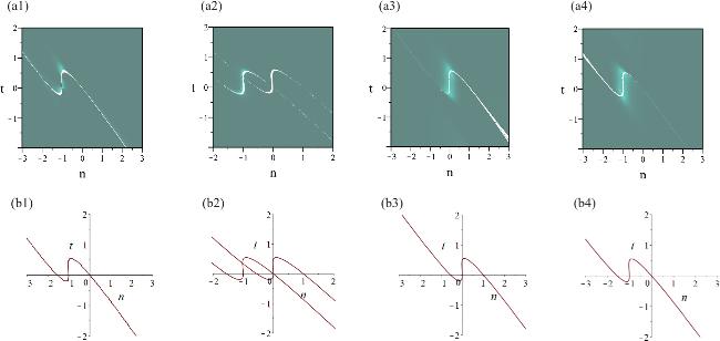
Figure 2. The structures of the first-order mixed rational-exponential solution equation ( |
For the purpose of investigating the limiting conditions of solution equation (11 ) in the period before and after collision, we assume that ξ1 is fixed, from which we get the following asymptotic states of solution equation (11 ):
α → + ∞ as t → + ∞:
$\begin{eqnarray*}\begin{array}{l}{\widetilde{a}}_{n}\to 1+\frac{49}{32}{{\rm{{\rm{sech}} }}}^{2}\left({\xi }_{1}+\frac{1}{2}\mathrm{ln}6\right), \\ {\widetilde{b}}_{n}\to 1-\frac{49}{16}{\rm{{\rm{sech}} }}\,\left({\xi }_{1}+\frac{1}{2}\mathrm{ln}6\right){\rm{{\rm{sech}} }}\left({\xi }_{1}+\frac{1}{2}\mathrm{ln}\frac{3}{4}\right),\\ {\widetilde{c}}_{n}\to 0,\,{\widetilde{d}}_{n}\to +\infty ,\end{array}\end{eqnarray*}$
α → − ∞ as t → − ∞:
$\begin{eqnarray*}\begin{array}{l}{\widetilde{a}}_{n}\to 1+\frac{49}{32}{{\rm{{\rm{sech}} }}}^{2}({\xi }_{1}+\frac{1}{2}\mathrm{ln}6), \\ {\widetilde{b}}_{n}\to 1-\frac{49}{16}{\rm{{\rm{sech}} }}\,\left({\xi }_{1}+\frac{1}{2}\mathrm{ln}6\right){\rm{{\rm{sech}} }}({\xi }_{1}+\frac{1}{2}\mathrm{ln}\frac{3}{4}),\\ \quad {\widetilde{c}}_{n}\to +\infty ,\,{\widetilde{d}}_{n}\to 0.\end{array}\end{eqnarray*}$
4.2. Second-order exact solutions
Case (i) Second-order exact rational solution
In the scenario where N = 1 and m = 2, indicating a requirement for two spectral parameters, we proceed solely with the Type 2 expansion for λ1 When N = 1, m = 2, that is to say, we need two spectral parameters, at this point, we only do the Type 2 expansion for λ1, while still do not perform the expansion for ${\lambda }_{2}=\frac{3}{2}$ with C1,2 = C3,2 = 0, C2,2 = − 1. Utilizing the (2, 1)-fold DT, the second-order exact rational solution can be formulated as specified below:
$\begin{eqnarray}\left\{\begin{array}{l}{\tilde{a}}_{n}=1-\displaystyle \frac{12{\alpha }^{4}+24{\alpha }^{3}+6{\alpha }^{2}+12t\alpha -6n}{{(2{\alpha }^{3}+3{\alpha }^{2}+n)}^{2}},\\ {\tilde{b}}_{n}=1+\displaystyle \frac{12{\alpha }^{4}-12n\alpha }{(2{\alpha }^{3}+3{\alpha }^{2}+n)(2{\alpha }^{3}-3{\alpha }^{2}+n)},\\ {\tilde{c}}_{n}=\displaystyle \frac{2{\alpha }^{3}-9{\alpha }^{2}+12\alpha +n}{2(2{\alpha }^{3}-3{\alpha }^{2}+n)}{{\rm{e}}}^{n\mathrm{ln}2-\tfrac{t}{2}},\\ {\tilde{d}}_{n}=0,\end{array}\right.\end{eqnarray}$
from which it is obvious that ${\widetilde{a}}_{n}$ possesses the singularity trajectory curve: 2α3 + 3α2 + n = 0, ${\widetilde{b}}_{n}$ possesses the singularity trajectory curve: 4α6 − 5α4 − 4tα3 + n2 = 0, while ${\widetilde{c}}_{n}$ possesses the singularity trajectory curve: 2α3 − 3α2 + n = 0. According to above results, we present the three-dimensional structures of solutions ${\widetilde{a}}_{n},\ {\widetilde{b}}_{n},\ {\widetilde{c}}_{n}$, as shown in figures 3(a1)-(a3), respectively, whose corresponding trajectory curves of ${\widetilde{a}}_{n},\ {\widetilde{b}}_{n},\ {\widetilde{c}}_{n}$ are displayed in figures 3(b1)–(b3), respectively. Meanwhile, we can easily know that ${\widetilde{a}}_{n}\to 1,\ {\widetilde{b}}_{n}\to 1$ as α → ± ∞, t → ± ∞ while ${\widetilde{c}}_{n}$ tends to 0 with t → + ∞ or ${\widetilde{c}}_{n}$ tends to +∞ with t → − ∞.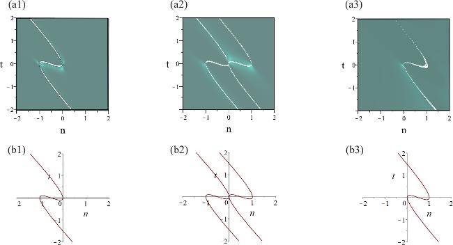
Figure 3. The structures of the second-order rational solution in equation ( |
Case (ii). Second-order exact combined rational-exponential solution
For deriving the second-order exact combined rational-exponential solution, we employ the Type 1 expansion solely to λ1, while no expansion is performed on λ2 with C1,2 = 0, C2,2 = − C3,2 = 1. Based on this, the formulation of the second-order exact rational-exponential solution can be deduced as
$\begin{eqnarray}\left\{\begin{array}{l}{\tilde{a}}_{n}=1-\displaystyle \frac{16({\alpha }^{2}-n)\cosh (2{\xi }_{2}+\mathrm{ln}2)+16\sqrt{5}\alpha \cosh (2{\xi }_{2}+\tfrac{1}{2}\mathrm{ln}\tfrac{4}{5})+8\sqrt{55}\cosh (2{\xi }_{2}+\tfrac{1}{2}\mathrm{ln}\tfrac{20}{11})-{M}_{1}}{32{N}_{1}^{2}},\\ {\tilde{b}}_{n}=1+\displaystyle \frac{16({\alpha }^{2}-n)\cosh 2{\xi }_{2}-16\sqrt{5}\alpha \sinh (2{\xi }_{2}-\tfrac{1}{2}\mathrm{ln}5)+8\sqrt{55}\cosh (2{\xi }_{2}+\tfrac{1}{2}\mathrm{ln}\tfrac{5}{11})-{M}_{2}}{16{N}_{1}{N}_{2}},\\ {\tilde{c}}_{n}=\displaystyle \frac{\sqrt{2}{{\rm{e}}}^{-t}(2\alpha \sinh {\xi }_{2}-3\cosh {\xi }_{2})}{2{N}_{2}},\\ {\tilde{d}}_{n}=\displaystyle \frac{8{{\rm{e}}}^{t}\sinh {\xi }_{2}}{{N}_{1}},\end{array}\right.\end{eqnarray}$
where $\begin{eqnarray*}\begin{array}{rcl}{M}_{1} & = & 9{\alpha }^{4}+18{\alpha }^{3}-18t{\alpha }^{2}-16{\alpha }^{2}\\ & & +31\alpha +9{n}^{2}-47n+62,\\ {M}_{2} & = & 9{\alpha }^{4}-18t{\alpha }^{2}-11{\alpha }^{2}-18n\alpha +68\alpha \\ & & +9{n}^{2}-52n+64,\\ {N}_{1} & = & ({\alpha }^{2}+n)\cosh ({\xi }_{2}+\frac{1}{2}\mathrm{ln}2)\\ & & -3\alpha \sinh ({\xi }_{2}+\frac{1}{2}\mathrm{ln}2)-\sqrt{2}\sinh {\xi }_{2},\\ {N}_{2} & = & ({\alpha }^{2}+n)\cosh ({\xi }_{2}-\frac{1}{2}\mathrm{ln}2)\\ & & -\sqrt{5}\alpha \sinh ({\xi }_{2}-\frac{1}{2}\mathrm{ln}2)+\sqrt{2}\sinh {\xi }_{2},\end{array}\end{eqnarray*}$
with ${\xi }_{2}=n\mathrm{ln}2+\frac{3}{4}t$. For observing the structures of solution equation (13 ), we display the three-dimensional structures shown in figures 4(a1)–(a4), while their corresponding trace curves are demonstrated in figures 4(b1)–(b4). Then, we give two types of limit states of solution equation (13 ):
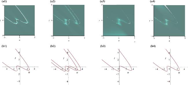
Figure 4. The structures of the second-order mixed rational-exponential solution equation ( |
Case (a) Similarly to the analysis of first-order mixed rational-exponential solution, we remain that ξ2 is fixed, then the limit states of solution equation (13 ) can be obtained:let α → + ∞ as t → + ∞: 13 ) can be deduced: let ξ2 → + ∞ as t → + ∞:
$\begin{eqnarray*}\begin{array}{l}{\widetilde{a}}_{n}\to 1+\frac{9}{8}{{\rm{{\rm{sech}} }}}^{2}\left({\xi }_{2}+\frac{1}{2}\mathrm{ln}2\right), \\ {\widetilde{b}}_{n}\to 1-\frac{9}{16}{\rm{{\rm{sech}} }}\,\,\left({\xi }_{2}-\frac{1}{2}\mathrm{ln}2\right){\rm{{\rm{sech}} }}\left({\xi }_{2}+\frac{1}{2}\mathrm{ln}2\right),\\ \quad {\widetilde{c}}_{n}\to 0,\,\,{\widetilde{d}}_{n}\to +\infty ,\end{array}\end{eqnarray*}$
let α → − ∞ as t → − ∞: $\begin{eqnarray*}\begin{array}{l}{\widetilde{a}}_{n}\to 1+\frac{9}{8}{{\rm{{\rm{sech}} }}}^{2}\left({\xi }_{2}+\frac{1}{2}\mathrm{ln}2\right),\, \\ {\widetilde{b}}_{n}\to 1-\frac{9}{16}{\rm{{\rm{sech}} }}\,\left({\xi }_{2}-\frac{1}{2}\mathrm{ln}2\right){\rm{{\rm{sech}} }}({\xi }_{2}+\frac{1}{2}\mathrm{ln}2),\\ {\widetilde{c}}_{n}\to +\infty ,\,{\widetilde{d}}_{n}\to 0,\end{array}\end{eqnarray*}$
Case (b) If we remain α fixed, another limit states of solution equation ( $\begin{eqnarray*}\begin{array}{l}{\widetilde{a}}_{n}\to 1-\frac{2({\alpha }^{2}+\sqrt{5}\alpha -n)+\sqrt{55}}{2{({\alpha }^{2}-3\alpha +n-\sqrt{2})}^{2}},\\ {\widetilde{b}}_{n}\to 1+\frac{2({\alpha }^{2}-\sqrt{5}\alpha -n)+\sqrt{55}}{({\alpha }^{2}-3\alpha +n-\sqrt{2})({\alpha }^{2}-\sqrt{5}\alpha +n+\sqrt{2})},\\ \quad {\widetilde{c}}_{n}\to 0,\,{\widetilde{d}}_{n}\to +\infty ,\end{array}\end{eqnarray*}$
let ξ2 → − ∞ as t → − ∞: $\begin{eqnarray*}\begin{array}{l}{\widetilde{a}}_{n}\to 1+\frac{2({\alpha }^{2}+\sqrt{5}\alpha -n)+\sqrt{55}}{2{({\alpha }^{2}+3\alpha +n+\sqrt{2})}^{2}},{\widetilde{b}}_{n}\to \\ \quad 1-\frac{2({\alpha }^{2}-\sqrt{5}\alpha -n)+\sqrt{55}}{({\alpha }^{2}+3\alpha +n+\sqrt{2})({\alpha }^{2}+\sqrt{5}\alpha +n-\sqrt{2})},\\ \quad {\widetilde{c}}_{n}\to +\infty ,\,{\widetilde{d}}_{n}\to 0.\end{array}\end{eqnarray*}$
4.3. The third-order exact rational solution
For the case where N = m = 1, the first third expansion of Type 1 for λ1 is essential for deriving the third-order exact solution, which can be listed as:
$\begin{eqnarray}\left\{\begin{array}{l}{\tilde{a}}_{n}=1-\displaystyle \frac{{\beta }_{1}}{{B}_{1}^{2}},\\ {\tilde{b}}_{n}=1+\displaystyle \frac{{\beta }_{2}}{{B}_{1}{B}_{2}},\\ {\tilde{c}}_{n}=\displaystyle \frac{(16{\alpha }^{3}-12\alpha +8n){{\rm{e}}}^{-t}}{{B}_{2}},\\ {\tilde{d}}_{n}=\displaystyle \frac{2({\alpha }^{4}-6{\alpha }^{3}+6(n+1){\alpha }^{2}-10n\alpha +3{n}^{2}){{\rm{e}}}^{t}}{{B}_{1}},\end{array}\right.\end{eqnarray}$
where 14 ), while their corresponding trace curves are demonstrated in figures 5(b1)–(b4).
$\begin{eqnarray*}\begin{array}{rcl}{B}_{1} & = & 2{\alpha }^{5}+5{\alpha }^{4}-4t{\alpha }^{3}-2(n+3){\alpha }^{2}\\ & & +2n(3n+4)\alpha -{n}^{2},\\ {B}_{2} & = & 2{\alpha }^{5}-9{\alpha }^{4}+4(n+3){\alpha }^{3}-2(7n+3){\alpha }^{2}\\ & & +6n(n+2)\alpha -7{n}^{2},\\ {\beta }_{1} & = & 20{\alpha }^{8}+48{\alpha }^{7}+(32n-60){\alpha }^{6}+224n{\alpha }^{5}\\ & & -(72{n}^{2}+84n-36){\alpha }^{4}+(80{n}^{2}-240n){\alpha }^{3}\\ & & +(116{n}^{2}+72){\alpha }^{2}-(144{n}^{2}+144n)\alpha \\ & & -36{n}^{4}-140{n}^{3}-84{n}^{2},\\ {\beta }_{2} & = & 20{\xi }^{8}-16{\alpha }^{7}+(32n-204){\alpha }^{6}+(224n+288){\alpha }^{5}\\ & & -(72{n}^{2}+580n-72){\alpha }^{4}+(272{n}^{2}-48n-144){\alpha }^{3}\\ & & +(-28{n}^{2}+360n){\alpha }^{2}-304{n}^{2}\alpha +36{n}^{4}+92{n}^{3},\end{array}\end{eqnarray*}$
from which it can be noted that ${\widetilde{a}}_{n}$ and ${\widetilde{d}}_{n}$ own the same singular trace curve B1 = 0, ${\widetilde{b}}_{n}$ exists two singular trace curves B1 = 0, B2 = 0, while ${\widetilde{c}}_{n}$ exists its singular trace curve B2 = 0. figures 5(a1)–(a4) display the three-dimensional structures of solution equation (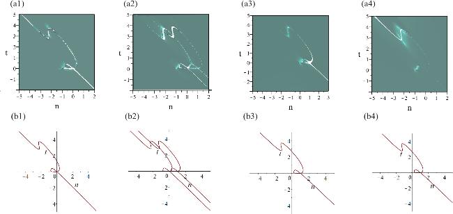
Figure 5. The structures of the third-order exact rational solution equation ( |
5. Conclusions
This study investigates a generalized Toda lattice equation (1 ) with four potentials linked to a 3 × 3 matrix spectrum problem. The main achievements are: (i) Transforming equation (1 ) into two distinct continuous equations via the continuous limit; (ii) Constructing a generalized (m, 3N − m)-fold DT of equation (1 ) for the first time; (iii) Deriving and meticulously analyzing singular exact rational and combined singular rational-exponential solutions, thoroughly analyzed and illustrated graphically, which are different from the usual soliton structures. The usual solitons are finite in amplitude and analytic, the solitons obtained in this paper have singularities along particular curves, and we have studied the singular trace curves of the solutions by asymptotic analysis. These results are innovative, which have not been considered in previous studies, and we expect they can provide new perspectives on wave propagation in one-dimensional nonlinear lattice dynamics.