


1. Introduction
Waveguide quantum electrodynamics (QED) is the study of light–matter interactions in confined waveguide structures, which plays a crucial role in quantum network construction and diverse quantum information processing tasks. In conventional waveguide systems, both natural and artificial atoms were typically treated as point-like dipoles. However, the demonstration of coherent coupling between a superconducting transmon qubit and surface acoustic waves in 2014 [1] invalidated the dipole approximation. In this configuration, the transmon’s dimensions become comparable to the acoustic wavelength, necessitating the consideration of nonlocal coupling effects through multiple interaction points, which give rise to giant atom quantum optics. Subsequently, the giant atom configuration was experimentally realized through coupling between transmon qubits or magnon spin ensembles and curved transmission lines, while being theoretically proposed in synthetic dimension frameworks [2–8]. The interference and retardation effects arising from nonlocal coupling in giant atom systems have attracted significant theoretical attention, revealing exotic phenomena including non-Markovian oscillations [9–11], decoherence-free interactions [12, 13], retardation effects [14, 15], Lamb shifts [16, 17], and chiral photonic population [18–22]. Furthermore, the interplay between topological photonic states and giant atoms has yielded novel effects such as chiral zero modes [15, 23], vacuum-like dressed states [24, 25], and broadband photonic reflection [26].
The waveguide serves as a quantum channel for photon propagation, offering an ideal carrier for quantum information transfer. Simultaneously, it provides a structured environment for quantum emitter manipulation. Among the most promising topics in waveguide QED are bound states, which emerge from the dressing of both atomic and photonic degrees of freedom. Conventional understanding suggests that such bound states typically reside outside the energy band. These bound states out of the continuum (BOCs) [27, 28] exhibit significant potential for applications including quantum coherence preservation [29], entanglement maintenance [30], quantum precision measurement realization [31, 32], as well as control of atomic evolution and photon propagation [33–38]. Recently, the bound state in the continuum (BIC) [39–41] has been attracting more and more attention due to its applications in enhancing light–matter interactions [42–44], generating low-threshold laser beams [45–47], enhancing nonlinear response [48, 49], realizing quantum sensing [50, 51], highly efficient wave guiding [52–55], etc.
In recent years, coupled resonator waveguides (CRWs) have been successfully fabricated in superconducting circuits, exhibiting excellent scalability and integration capabilities [56–58]. The cosine-type dispersion relation of CRWs offers new opportunities for manipulating light–matter interactions. In particular, BOCs and BICs in atom–CRW systems have recently garnered significant research attention [28, 36, 37, 59–63]. Nevertheless, while most existing studies focus on bound-state properties, systematic investigations of methods to control their frequency and wave function remain notably absent.
To address these challenges, we propose a scheme for engineering both BOCs and BICs through nonlocal coupling of a giant atom to a CRW at two distinct sites. This study specifically investigates the phase-controlled manipulation of BOCs and BICs via the coupling phase between the giant atom and CRW. We derive analytical expressions for: (i) the conditions under which BOCs exist, (ii) the eigenfrequency of BICs, and (iii) their corresponding photonic distribution profiles. Furthermore, we reveal a novel quantum beat phenomenon arising from BIC–BOC oscillations—a distinctive feature absent from conventional small atom systems.
2. Model
As schematically shown in figure 1, a single giant atom is connected to the CRW at the zeroth and Nth sites. The Hamiltonian of the structure in real space reads H=HA+Hc+HI, where (ℏ=1):
$\begin{eqnarray}{H}_{A}={\rm{\Omega }}| {\rm{e}}\rangle \langle {\rm{e}}| ,\end{eqnarray}$
$\begin{eqnarray}{H}_{c}={\omega }_{c}\displaystyle \sum _{j}{a}_{j}^{\dagger }{a}_{j}-\xi \displaystyle \sum _{j}({a}_{j+1}^{\dagger }{a}_{j}+{a}_{j}^{\dagger }{a}_{j+1}),\end{eqnarray}$
$\begin{eqnarray}{H}_{I}=g[({a}_{0}^{\dagger }+{a}_{N}^{\dagger }{{\rm{e}}}^{{\rm{i}}\phi }){\sigma }_{-}+{\rm{H}}{\rm{.}}{\rm{c}}{\rm{.}}].\end{eqnarray}$
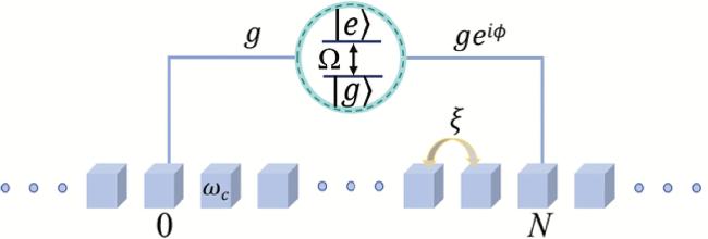
Figure 1. Sketch of the waveguide QED setup, where a giant atom is coupled to a coupled resonator waveguide via the zeroth and Nth sites. |
Here, HA and Hc are the Hamiltonians of the giant atom and the CRW, respectively, and HI represents their interaction. We have used the rotating-wave and dipole approximations at each coupling point between the giant atom and the CRW. Ω is the transition frequency of the giant atom between the ground state ∣g⟩ and the excited state ∣e⟩. ωc is the intrinsic frequency of each resonator in the CRW. aj is the annihilation operator of the jth resonator in the CRW. σ+ = ∣e⟩⟨g∣ is the raising operator of the giant atom. ξ is the hopping strength between the nearest resonators in the CRW. g is the real coupling strength between the giant atom and the connected resonator. We have assumed that the coupling phase in the left leg is zero, while that for the right leg is φ. For the convenience of calculation, we will shift the energy level of the Hamiltonian and set ωc to zero in what follows.
We model the CRW as an infinite periodic array of resonators, which ensures strict translational invariance in the system. Using the Fourier transformation ${a}_{k}^{\dagger }={\sum }_{j}{a}_{j}^{\dagger }\exp (-{\rm{i}}kj)/\sqrt{{N}_{c}}$, where Nc → ∞ is the length of the waveguide, we can express the Hamiltonian of the CRW Hc as ${H}_{c}={\sum }_{k}{\omega }_{k}{a}_{k}^{\dagger }{a}_{k}$, where the dispersion relation satisfies ${\omega }_{k}=-2\xi \cos k$. This states that the single-photon energy band possesses a width of 4ξ. In terms of the operator ak, the interaction Hamiltonian becomes
$\begin{eqnarray}{H}_{I}=\displaystyle \frac{g}{\sqrt{{N}_{c}}}\displaystyle \sum _{k}[{a}_{k}^{\dagger }{\sigma }_{-}(1+{{\rm{e}}}^{{\rm{i}}({kN}+\phi )})+{\rm{H}}{\rm{.}}{\rm{c}}{\rm{.}}],\end{eqnarray}$
It is obvious that the coupling amplitude between the giant atom and its resonant mode in the CRW is $\begin{eqnarray}G(K,\phi )=\displaystyle \frac{g}{\sqrt{{N}_{c}}}(1+{{\rm{e}}}^{{\rm{i}}(KN+\phi )}),\end{eqnarray}$
which depends on φ, while K satisfies ${\rm{\Omega }}=-2\xi \cos K$.In figures 2(a) and (b), we numerically calculate the energy spectrum of the system within the single-excitation subspace for varying atomic resonant frequencies and coupling phases φ. As the coupling strength g increases, the topmost and bottommost energy levels (represented by red solid curves) progressively separate from the continuous spectrum, forming BOCs. These states emerge due to the broken translational symmetry in the waveguide caused by the giant atom coupling. Similar BOCs have been previously reported in CRW systems coupled to traditional small atoms [28, 33, 37]. At small g values, the bound-state nature of these two levels cannot be conclusively determined from figures 2(a) and (b); therefore, we will provide a detailed analysis in the following section. Additionally, we identify a single BIC, indicated by the blue line in the figure. This BIC remains resonant with the giant atom’s frequency and originates from destructive interference between the two atom–waveguide coupling sites. The fundamental characteristics distinguishing these states as genuine bound states will be systematically examined in subsequent discussions.
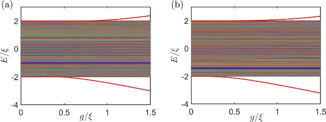
Figure 2. Energy diagram of the giant atom–CRW coupled system. The thick blue line in the continuum represents the BIC, while the red curves represent the BOC. The parameters are set to Ω = − ξ, N = 6, φ = π in (a) and ${\rm{\Omega }}=-\sqrt{2}\xi ,N=12,\phi =0$ in (b). |
To investigate these states more thoroughly, we resort to the single-photon wave function ansatz of
$\begin{eqnarray}\left|\phi \right\rangle =\alpha {\sigma }_{+}| G\rangle +\displaystyle \sum _{k}{\beta }_{k}{a}_{k}^{\dagger }\left|G\right\rangle ,\end{eqnarray}$
where ∣G⟩ denotes that both the giant atom and the waveguide are in their ground states. According to the Schrödinger equation H∣φ⟩ = E∣φ⟩, we can obtain $\begin{eqnarray}E-{\rm{\Omega }}=Y(E),\end{eqnarray}$
$\begin{eqnarray}\displaystyle \frac{{\beta }_{k}}{\alpha }=\displaystyle \frac{1}{\sqrt{{N}_{c}}}\displaystyle \frac{g+g{{\rm{e}}}^{{\rm{i}}(kN+\phi )}}{E+2\xi \cos k},\end{eqnarray}$
where the auxiliary function Y(E) is defined as $\begin{eqnarray}Y(E)\equiv \displaystyle \frac{{g}^{2}}{\pi }{\int }_{-\pi }^{\pi }\displaystyle \frac{1+\cos (kN+\phi )}{E+2\xi \cos k}{\rm{d}}k.\end{eqnarray}$
3. Bound states out of the continuum
In this section, we will investigate the BOCs of the system by solving the energy equation in equation (7 ) in the regime of ∣E∣ > 2ξ. For simplicity, we denote the topmost and bottommost states (eigenenergies) by ∣EU⟩ (EU) and ∣EL⟩ (EL), respectively. After the detailed calculations shown in Appendix A , we find that the corresponding energy satisfies the transcendental equation EU(L) − Ω = Y(EU(L)), where
$\begin{eqnarray}Y({E}_{U})=\frac{{g}^{2}}{\xi }\frac{1+{\left[-\frac{{E}_{U}}{2\xi }+\sqrt{{\left(\frac{{E}_{U}}{2\xi }\right)}^{2}-1}\right]}^{N}\cos \phi }{\sqrt{{\left(\frac{{E}_{U}}{2\xi }\right)}^{2}-1}},\end{eqnarray}$
$\begin{eqnarray}Y({E}_{L})=-\frac{{g}^{2}}{\xi }\frac{1+{\left[-\frac{{E}_{L}}{2\xi }-\sqrt{{\left(\frac{{E}_{L}}{2\xi }\right)}^{2}-1}\right]}^{N}\cos \phi }{\sqrt{{\left(\frac{{E}_{L}}{2\xi }\right)}^{2}-1}}.\end{eqnarray}$
Y(EU) and Y(EL) are monotonically decreasing functions in the regime of EU > 2ξ and EL < − 2ξ, respectively. Therefore, the conditions for the existence of the upper and lower BOCs can be written as [38] $\begin{eqnarray}\mathop{\mathrm{lim}}\limits_{{E}_{U}\to 2\xi }Y({E}_{U})\gt 2\xi -{\rm{\Omega }},\end{eqnarray}$
$\begin{eqnarray}\mathop{\mathrm{lim}}\limits_{{E}_{L}\to -2\xi }Y({E}_{L})\lt -2\xi -{\rm{\Omega }}.\end{eqnarray}$
In table 1, we list the above conditions, focusing on the atom–waveguide coupling strength g for different values of φ. Here, we use the notation ‘√’ to indicate that the corresponding BOC always exists, regardless of the atom–waveguide coupling strength.Table 1. The conditions for the existence of the BOC. Here, n is taken to be integer. √ denotes that the corresponding BOC always exists, regardless of the atom–waveguide coupling strength g. |
| EU | φ = (2n + 1)π | φ = 2nπ | φ = other |
|---|---|---|---|
| N = 2n + 1 | √ | ${g}^{2}\gt \frac{2{\xi }^{2}-{\rm{\Omega }}\xi }{N}$ | √ |
| | |||
| N = 2n | ${g}^{2}\gt \frac{2{\xi }^{2}-{\rm{\Omega }}\xi }{N}$ | √ | √ |
| | |||
| EL | φ = (2n + 1)π | φ = 2nπ | φ = other |
| | |||
| N = 2n + 1 | ${g}^{2}\gt \frac{2{\xi }^{2}+{\rm{\Omega }}\xi }{N}$ | √ | √ |
| | |||
| N = 2n | ${g}^{2}\gt \frac{2{\xi }^{2}+{\rm{\Omega }}\xi }{N}$ | √ | √ |
Based on the conditions listed in table 1, we further examine the photonic distributions of the topmost and bottommost states in figures 2(a) and (b) (both for even N), respectively. For the weak coupling strength g = 0.1ξ, both EU and EL exhibit extended characteristics (see figure 3(a)) when φ = π, indicating that neither state constitutes a bound state. Conversely, the results for φ = 0 in figure 3(c) demonstrate that the photonic amplitudes decay slowly beyond the region covered by the giant atom, which represents a characteristic bound-state feature. To obtain tighter bound states, we plot the results for larger g in figures 3(b) and (d), where photons become strongly localized near the two atom–waveguide coupling sites for both φ = π and φ = 0. Additionally, we present results for odd N in figures 3(e-h). When φ = π, the topmost state forms a bound state, while the bottommost state does not, as shown in figure 3(e). Conversely, when φ = 0, we observe the opposite behavior compared to the φ = π case, as demonstrated in figure 3(g). Under strong atom–waveguide coupling conditions, the photonic distributions in figures 3(f) and (h) reveal that both states become well-defined bound states, exhibiting similar characteristics to those observed for even N. These findings align with the conditions summarized in table 1. The presence of the coupling phase φ challenges the conventional conclusion that the bottommost state must necessarily be a BOC in giant atom–CRW systems [38].
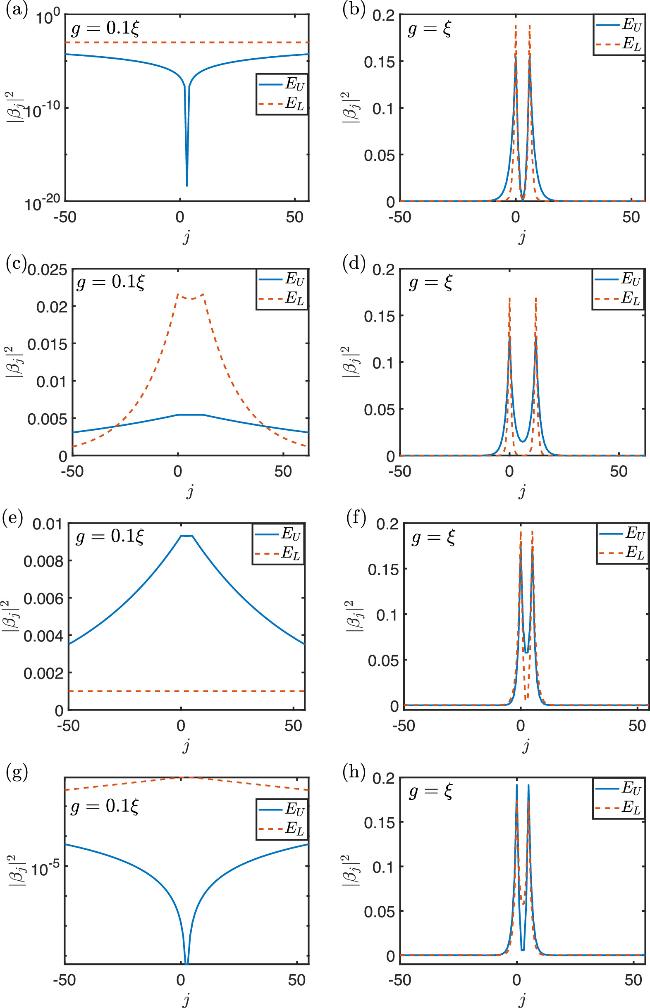
Figure 3. The photonic population in the waveguide for the BOCs ∣EU⟩ and ∣EL⟩. The parameters are set to (a), (b) Ω = − ξ, N = 6, φ = π. (c), (d) ${\rm{\Omega }}=-\sqrt{2}\xi ,N=12,\phi =0$. (e), (f) Ω = 0, N = 5, φ = π. (g), (h) Ω = 0, N = 5, φ = 0. |
4. Bound state in the continuum
In the previous section, we discussed the BOCs in the giant atom–waveguide coupled system. We now turn to the continuous band. In figures 4(a) and (b), we plot the density of states (DOS), ρ, within the energy range −2ξ < E < 2ξ when the giant atom is decoupled from its resonant mode in the waveguide; that is, ∣G(K, φ)∣2 = 0. A single peak appears in both figures, precisely located at the atomic frequency Ω. As derived in Appendix B , we demonstrate that E = Ω satisfies the energy equation (equation (7 )), corresponding to a discrete energy level. In figure 2, this energy level is indicated by the blue line, representing the BIC, as will be verified through both numerical and analytical approaches below.
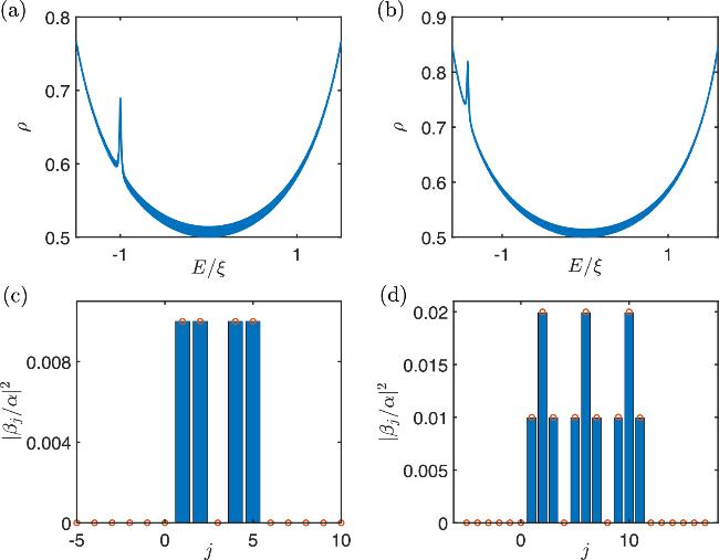
Figure 4. The density of states (a), (b) and the photonic distribution (c), (d) of the giant atom–waveguide coupled system. The parameters are set to g = 0.1ξ, ωc = 0 and Ω = − ξ, N = 6, φ = π in (a) and (c), and ${\rm{\Omega }}=-\sqrt{2}\xi ,N=12,\phi =0$ in (b) and (d). |
With the assistance of the inverse Fourier transformation B ):
$\begin{eqnarray}{\beta }_{j}=\frac{1}{\sqrt{{N}_{c}}}\displaystyle \sum _{k}{\beta }_{k}{{\rm{e}}}^{-{\rm{i}}kj},\end{eqnarray}$
we can obtain the photonic distribution for the BIC (E = Ω) as follows (see Appendix $\begin{eqnarray}\frac{{\beta }_{j}}{\alpha }=\left\{\begin{array}{l}0,\quad j\lt 0\,\,\,\rm{and}\,\,\,j\gt N\quad \\ \frac{2g\sin (Kj)}{\sqrt{4{\xi }^{2}-{{\rm{\Omega }}}^{2}}},\quad 0\leqslant j\leqslant N\quad \end{array}\right..\end{eqnarray}$
This indicates that photons in the waveguide become confined within the spatial region covered by the giant atom, thus constituting the BIC. The BIC differs fundamentally from other continuum states where photons are distributed throughout the entire waveguide.
In figures 4(c) and (d), we present the standing-wave photonic distribution of the BIC. The solid bars denote numerical results obtained through direct Hamiltonian diagonalization in the single-excitation subspace, while empty circles represent analytical results derived from equation (15 ). For the parameter choice Ω/ξ = − 1, we obtain K = π/3. Figure 4(c) reveals photon occupation at sites j = 1, 2, 4, and 5 but not at j = 3. Conversely, for the parameters ${\rm{\Omega }}/\xi =-\sqrt{2}$, φ = 0, N = 12, the photon distribution vanishes between the giant atom’s coupling sites at positions j = 4m (m = 0, 1, 2, and 3). These results demonstrate that both the BIC frequency and its photonic distribution can be controlled by adjusting the giant atom’s size, transition frequency, and waveguide coupling phase.
5. BIC–BOC transition dynamics
In this section, we investigate the dynamics of the system for both the atomic and photonic counterparts by setting the initial state to ∣ψ(0)⟩ = σ+∣G⟩, where the giant atom is in its excited state while all the resonators are in their ground states.
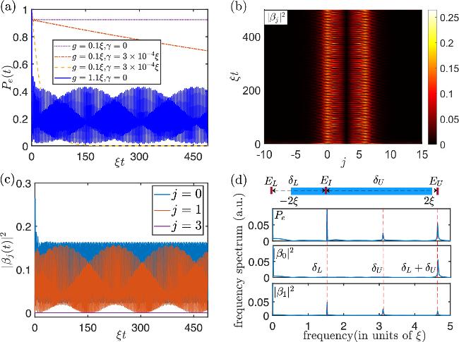
In figure 5, we numerically illustrate the dynamical evolution of the system, governed by $| \psi (t)\rangle =\exp (-{\rm{i}}Ht)| \psi (0)\rangle $. As the blue solid curve shows in figure 5(a), we observe that Pe = ∣⟨ψ(t)∣σ+∣G⟩∣2 exhibits a slowly varying envelope and fast oscillation within each envelope for the parameters Ω = − ξ, N = 6, φ = π, g = 1.1ξ, in which case the energy spectrum is as shown in figure 2(a). The photonic dynamics $| {\beta }_{j}{| }^{2}\,=| \langle \psi (t)| {a}_{j}^{\dagger }| G\rangle {| }^{2}$ is shown in figure 5(b). The photon emitted by the giant atom is nearly completely trapped inside the covered region. We further plot the evolution of the photonic distribution in the resonators j = 0, 1, and 3 in figure 5(c). The photon is never excited in the third resonator; in other words, ∣β3∣ = 0 during the time evolution. For j = 1, we find a similar quantum beat phenomenon with the atomic dynamics (the same result for j = 2 is not shown in the figure). For j = 0, a single high oscillation frequency is observed.
Figure 5. The dynamical evolution of the system. (a) The dynamics of the atomic population in its excited states. ωc = 0, Ω = − ξ, N = 4, φ = π for the yellow dashed curve and ωc = 0, Ω = − ξ, N = 6, φ = π for the other curves. (b) and (c) The dynamics of the photonic distribution. (d) The frequency spectra of the atomic and photonic dynamical evolutions obtained by numerical Fourier transformations from the time domain to the frequency domain. (b)–(d) The parameters are set to ωc = 0, Ω = − ξ, g = 1.1ξ, N = 6, φ = π. |
To understand the above dynamical process, we write the initial state as
$\begin{eqnarray}| \psi (0)\rangle ={c}_{U}| {\phi }_{U}\rangle +{c}_{I}| {\phi }_{I}\rangle +{c}_{L}| {\phi }_{L}\rangle +\displaystyle \sum _{k}{c}_{k}| {\phi }_{k}\rangle ,\end{eqnarray}$
where ∣φU⟩ and ∣φL⟩ are the upper and lower BOCs with eigenenergies of EU and EL, respectively, and ∣φI⟩ is the BIC with an eigenenergy of EI. Here, ∣φk⟩ is the kth propagating photonic mode in the waveguide, and the C-numbers cm (m = U, I, L, k) denote the corresponding amplitudes. Building on the exact numerical results given in figure 2(a), the eigenenergy of the system is illustrated by the diagram at the top of figure 5(d). Here, the continuous band, which is located in the regime of [ − 2ξ, 2ξ] is represented by the horizontal blue bar, while the BIC and BOCs are indicated by vertical dark red bars. It is well known that, due to the interference effect, the propagating modes do not contribute to the atomic dynamics when the evolution time is long enough [63, 64]. Therefore, in the long time limit, we have $\begin{eqnarray}\begin{array}{rcl}{P}_{{\rm{e}}}(t) & = & | {{\rm{e}}}^{-{\rm{i}}{E}_{L}t}{c}_{L}^{2}+{{\rm{e}}}^{-{\rm{i}}{E}_{I}t}{c}_{I}^{2}+{{\rm{e}}}^{-{\rm{i}}{E}_{U}t}{c}_{U}^{2}{| }^{2}\\ & = & | {{\rm{e}}}^{{\rm{i}}{\delta }_{L}t}{c}_{L}^{2}+{c}_{I}^{2}+{{\rm{e}}}^{-{\rm{i}}{\delta }_{U}t}{c}_{U}^{2}{| }^{2},\end{array}\end{eqnarray}$
$\begin{eqnarray}| {\beta }_{j}(t){| }^{2}=| {{\rm{e}}}^{-{\rm{i}}{\delta }_{U}t}{c}_{U}{d}_{U,j}+{{\rm{e}}}^{{\rm{i}}{\delta }_{L}t}{c}_{L}{d}_{L,j}+{c}_{I}{d}_{I,j}{| }^{2},\end{eqnarray}$
where δL = EI − EL and δU = EU − EI are the detunings between the BOCs and the BIC, while ${d}_{\alpha ,j}=\langle {\phi }_{\alpha }| {a}_{j}^{\dagger }| G\rangle (\alpha =U,I,L)$ denotes the photonic excitation amplitude at the jth resonator of the waveguide when the system is in the bound state ∣φα⟩.To further investigate the dynamical properties of the system, we apply the numerical fast Fourier transformation technique to obtain the frequency spectra for Pe and ∣βj∣2 (j = 0, 1) shown in the lower three panels of figure 5(d). We observe three significant peaks for Pe and ∣β1∣2, which are located at the frequencies δL, δU, and δU + δL, in agreement with the analytical expression in equations (17 ) and (18 ). This implies that the dynamics of the giant atom is induced by the oscillations between the single BIC and the two BOCs (contributing the peaks located at δU and δL) and between the two BOCs (contributing the peak located at δU + δL). On the contrary, we only find a single peak located at the frequency of δU + δL in the spectrum of ∣β0∣2. This can also be explained by the analytical expression in equation (18 ), in which there only exists a single nonzero frequency component at δU + δL (since dI,0 = 0), as shown in figure 4(c). This further indicates that the oscillation between the two BOCs contributes to the photonic dynamics in the zeroth cavity.
In the above, we have demonstrated that the presence of a BIC effectively protects the giant atom from undergoing exponential decay into the structured environment provided by the CRW. This protective effect becomes more significant in the weak coupling regime; for instance, when the atom–waveguide coupling strength is as small as g = 0.1ξ, the atomic oscillations are completely suppressed, as shown by the purple dotted curve in figure 5(a). Moreover, this suppression of atomic dissipation remains robust even in the presence of intrinsic spontaneous emission of the giant atom. A comparison between the cases with and without BICs—represented by the orange dot-dashed and yellow dashed curves, respectively—clearly illustrates that the BIC significantly slows down the atomic decay. Therefore, the BIC mechanism offers a powerful means of preserving the atomic population, even when spontaneous emission is taken into account.
6. Conclusions
In this paper, we studied the engineering of BOCs and the BIC in a one-dimensional QED setup with a giant atom. We found that the number of BOCs and the BIC can be controlled on demand by the size of the giant atom and the coupling phase to the waveguide. We also proved that the BIC is exactly resonant with the frequency of the giant atom. Induced by BIC-BOC oscillations, both atomic and photonic dynamics are characterized by a quantum beat phenomenon.
The giant atom can be realized using superconducting transmon qubits, and CRWs with up to tens of sites [58, 65] have also been fabricated in superconducting circuits. In these experimental implementations, the achievable parameters fall within the regime of g ≪ ξ ≈ 100 − 200 MHz. Therefore, our predicted dynamical behavior remains observable, even when the giant atom experiences spontaneous emission with a lifetime of T1 = 10 μs [66].
Beyond the specific setting considered in this work, our investigation can be extended to systems consisting of multiple giant atoms or a single giant atom coupled to the waveguide through multiple sites with on-demand coupling strengths and phases. In these more complex configurations, both the BIC and BOC warrant in-depth investigation, which may enable the design of desired dynamical processes for quantum information applications.
Appendix A Bound state out of the continuum
In equations (7 ), (10 ), and (11 ) of the main text, we gave the transcendental equations for the energies of the bound states. In this appendix, we give a detailed derivation.
We begin with the Hamiltonian in equation (4 ) and the wave function in equation (6 ). The Schödinger equation H∣φ⟩ = E∣φ⟩ yields
$\begin{eqnarray}\begin{array}{rcl}\alpha (E-{\rm{\Omega }}) & = & \displaystyle \frac{g}{\sqrt{{N}_{c}}}\displaystyle \sum _{k}{\beta }_{k}[1+{{\rm{e}}}^{-{\rm{i}}(kN+\phi )}],\\ (E+2\xi \cos k){\beta }_{k} & = & \displaystyle \frac{g\alpha }{\sqrt{{N}_{c}}}[1+{{\rm{e}}}^{{\rm{i}}(kN+\phi )}].\end{array}\end{eqnarray}$
By eliminating α and βk, we obtain the equation for the eigenenergy E, as follows:7 ) in the main text. We now perform the integration to calculate Y(E) by introducing a new variable z = eik. We obtain10 ) and (11 ) in the main text.
$\begin{eqnarray}E-{\rm{\Omega }}=Y(E)\equiv \displaystyle \frac{{g}^{2}}{\pi }{\int }_{-\pi }^{\pi }\displaystyle \frac{1+\cos (kN+\phi )}{E+2\xi \cos k}{\rm{d}}k,\end{eqnarray}$
which is equation ( $\begin{eqnarray}\begin{array}{rcl}Y(E) & = & \displaystyle \frac{{g}^{2}}{\pi }{\int }_{-\pi }^{\pi }\displaystyle \frac{1+\cos (kN+\phi )}{E+2\xi \cos k}{\rm{d}}k\\ & = & \displaystyle \frac{{g}^{2}}{2\pi }{\int }_{-\pi }^{\pi }\displaystyle \frac{2+{{\rm{e}}}^{{\rm{i}}(kN+\phi )}+{{\rm{e}}}^{{\rm{i}}(kN-\phi )}}{E+\xi ({{\rm{e}}}^{{\rm{i}}k}+{{\rm{e}}}^{-{\rm{i}}k})}{\rm{d}}k\\ & = & \displaystyle \frac{{g}^{2}}{2{\rm{i}}\pi \xi }{\oint }_{| z| =1}\displaystyle \frac{2+{z}^{N}{{\rm{e}}}^{{\rm{i}}\phi }+{z}^{N}{{\rm{e}}}^{-{\rm{i}}\phi }}{{z}^{2}+Ez/\xi +1}{\rm{d}}z\\ & = & \displaystyle \frac{{g}^{2}}{2{\rm{i}}\pi \xi }{\oint }_{| z| =1}\displaystyle \frac{2+{z}^{N}{{\rm{e}}}^{{\rm{i}}\phi }+{z}^{N}{{\rm{e}}}^{-{\rm{i}}\phi }}{(z-{z}_{1})(z-{z}_{2})}{\rm{d}}z,\end{array}\end{eqnarray}$
where ${z}_{1}=-(E/2\xi )+\sqrt{{(E/2\xi )}^{2}-1}$ and ${z}_{2}=-(E/2\xi )\,-\sqrt{{(E/2\xi )}^{2}-1}$. In the regime of ∣E∣ > 2ξ, we have $\begin{eqnarray}\begin{array}{rcl}Y({E}_{U}) & = & \frac{{g}^{2}}{\xi }\frac{2+2{z}_{1}^{N}\cos \phi }{{z}_{1}-{z}_{2}}\\ & = & \frac{{g}^{2}}{\xi }\frac{1+{\left[-\frac{{E}_{U}}{2\xi }+\sqrt{{\left(\frac{{E}_{U}}{2\xi }\right)}^{2}-1}\right]}^{N}\cos \phi }{\sqrt{{\left(\frac{{E}_{U}}{2\xi }\right)}^{2}-1}},\end{array}\end{eqnarray}$
$\begin{eqnarray}\begin{array}{rcl}Y({E}_{L}) & = & \frac{{g}^{2}}{\xi }\frac{2+2{z}_{2}^{N}\cos \phi }{{z}_{2}-{z}_{1}}\\ & = & -\frac{{g}^{2}}{\xi }\frac{1+{\left[-\frac{{E}_{L}}{2\xi }-\sqrt{{\left(\frac{{E}_{L}}{2\xi }\right)}^{2}-1}\right]}^{N}\cos \phi }{\sqrt{{\left(\frac{{E}_{L}}{2\xi }\right)}^{2}-1}},\end{array}\end{eqnarray}$
where we have assumed EU > 2ξ and EL < − 2ξ, which represent the upper and lower BOCs, respectively. Therefore, we obtain equations (Appendix B Bound state in the continuum
In this appendix, we give the detailed derivation of the energy and the wave function of the BIC.
First, we prove that E = Ω is a solution of the transcendental equation (7 ) in the main text' in other words, we prove that
$\begin{eqnarray}Y({\rm{\Omega }})=\displaystyle \frac{{g}^{2}}{\pi }{\int }_{-\pi }^{\pi }\displaystyle \frac{1+\cos (kN+\phi )}{{\rm{\Omega }}+2\xi \cos k}{\rm{d}}k\end{eqnarray}$
is always zero. To this end, we rewrite Y(Ω) as $\begin{eqnarray}\begin{array}{rcl}Y({\rm{\Omega }}) & = & \displaystyle \frac{{g}^{2}}{\pi }{\int }_{-\pi }^{\pi }\displaystyle \frac{1+\cos (kN+\phi )}{{\rm{\Omega }}+2\xi \cos k}{\rm{d}}k\\ & = & \displaystyle \frac{{g}^{2}}{2\pi }{\int }_{-\pi }^{\pi }\displaystyle \frac{2+{{\rm{e}}}^{{\rm{i}}(kN+\phi )}+{{\rm{e}}}^{-{\rm{i}}(kN+\phi )}}{{\rm{\Omega }}+\xi ({{\rm{e}}}^{{\rm{i}}k}+{{\rm{e}}}^{-{\rm{i}}k})}{\rm{d}}k\\ & = & \displaystyle \frac{{g}^{2}}{2{\rm{i}}\xi \pi }{\oint }_{| z| =1}\displaystyle \frac{2{z}^{N}+{z}^{2N}{{\rm{e}}}^{{\rm{i}}\phi }+{{\rm{e}}}^{-{\rm{i}}\phi }}{(z-{z}_{1})(z-{z}_{2}){z}^{N}}{\rm{d}}z,\end{array}\end{eqnarray}$
where ${z}_{1,2}=-({\rm{\Omega }}/2\xi )\pm {\rm{i}}\sqrt{1-{({\rm{\Omega }}/2\xi )}^{2}}={{\rm{e}}}^{\pm {\rm{i}}K}$, which satisfies ∣z1,2∣ = 1. Applying the residue theorem to solve the above integral, only the N-order singular points (z = 0) need to be considered. Therefore, $\begin{eqnarray}\begin{array}{rcl}Y({\rm{\Omega }}) & = & \displaystyle \frac{{g}^{2}}{\xi }\displaystyle \frac{1}{(N-1)!}\displaystyle \frac{{{\rm{d}}}^{N-1}}{{\rm{d}}{z}^{N-1}}{\left.\left[\displaystyle \frac{2{z}^{N}+{z}^{2N}{{\rm{e}}}^{{\rm{i}}\phi }+{{\rm{e}}}^{-{\rm{i}}\phi }}{(z-{z}_{1})(z-{z}_{2})}\right]\right|}_{z=0}\\ & = & \displaystyle \frac{{g}^{2}{{\rm{e}}}^{-{\rm{i}}\phi }}{2{\rm{i}}\xi \sqrt{1-{({\rm{\Omega }}/2\xi )}^{2}}}({z}_{2}^{-N}-{z}_{1}^{-N})\\ & = & \displaystyle \frac{{g}^{2}}{2{\rm{i}}\xi \sqrt{1-{({\rm{\Omega }}/2\xi )}^{2}}}({{\rm{e}}}^{-{\rm{i}}(KN+\phi )}-{{\rm{e}}}^{{\rm{i}}(KN-\phi )})\\ & = & \displaystyle \frac{{g}^{2}}{2{\rm{i}}\xi \sqrt{1-{({\rm{\Omega }}/2\xi )}^{2}}}({G}^{* }(K,\phi )-{G}^{* }(-K,\phi ))\\ & = & 0,\end{array}\end{eqnarray}$
where we have used the condition G*(K, φ) = G*(− K, φ) = 0 for the BIC.Next, we study the wave function of the BIC. From equation (19 ), we have
$\begin{eqnarray}\displaystyle \frac{{\beta }_{k}}{\alpha }=\displaystyle \frac{g}{\sqrt{{N}_{c}}}\displaystyle \frac{1+{{\rm{e}}}^{{\rm{i}}(kN+\phi )}}{E+2\xi \cos k}.\end{eqnarray}$
Going back into the real space, we have $\begin{eqnarray}\begin{array}{rcl}\displaystyle \frac{{\beta }_{j}}{\alpha } & = & \displaystyle \frac{g}{{N}_{c}}\displaystyle \sum _{k}\displaystyle \frac{[1+{{\rm{e}}}^{{\rm{i}}(kN+\phi )}]{{\rm{e}}}^{-{\rm{i}}kj}}{{\rm{\Omega }}+2\xi \cos k}\\ & = & \displaystyle \frac{g}{2\pi }{\int }_{-\pi }^{\pi }\displaystyle \frac{[1+{{\rm{e}}}^{{\rm{i}}(kN+\phi )}]{{\rm{e}}}^{-{\rm{i}}kj}}{{\rm{\Omega }}+2\xi \cos k}{\rm{d}}k\\ & = & \displaystyle \frac{g}{2{\rm{i}}\pi \xi }{\oint }_{| z| =1}\displaystyle \frac{1+{z}^{N}{{\rm{e}}}^{{\rm{i}}\phi }}{(z-{z}_{1})(z-{z}_{2}){z}^{j}}{\rm{d}}z.\end{array}\end{eqnarray}$
When j < 0, there is no singular point in the integral domain, so
$\begin{eqnarray}\displaystyle \frac{{\beta }_{j}}{\alpha }=\displaystyle \frac{g}{2{\rm{i}}\pi \xi }{\oint }_{| z| =1}\displaystyle \frac{1+{z}^{N}{{\rm{e}}}^{{\rm{i}}\phi }}{(z-{z}_{1})(z-{z}_{2}){z}^{j}}{\rm{d}}z=0.\end{eqnarray}$
When 0 ≤ j ≤ N,
$\begin{eqnarray}{\oint }_{| z| =1}\displaystyle \frac{{z}^{N}{{\rm{e}}}^{{\rm{i}}\phi }}{(z-{z}_{1})(z-{z}_{2}){z}^{j}}{\rm{d}}z=0.\end{eqnarray}$
Therefore, we obtain $\begin{eqnarray}\begin{array}{rcl}\displaystyle \frac{{\beta }_{j}}{\alpha } & = & \displaystyle \frac{g}{2{\rm{i}}\pi \xi }{\oint }_{| z| =1}\displaystyle \frac{1}{(z-{z}_{1})(z-{z}_{2}){z}^{j}}{\rm{d}}z\\ & = & \displaystyle \frac{g}{\xi (j-1)!}\displaystyle \frac{{d}^{j-1}}{d{z}^{j-1}}{\left.\left[\displaystyle \frac{1}{(z-{z}_{1})(z-{z}_{2})}\right]\right|}_{z=0}\\ & = & \displaystyle \frac{g}{2{\rm{i}}\xi \sqrt{1-{({\rm{\Omega }}/2\xi )}^{2}}}({z}_{1}^{j}-{z}_{2}^{j})\\ & = & \displaystyle \frac{g}{2{\rm{i}}\xi \sqrt{1-{({\rm{\Omega }}/2\xi )}^{2}}}({{\rm{e}}}^{{\rm{i}}Kj}-{{\rm{e}}}^{-{\rm{i}}Kj})\\ & = & \displaystyle \frac{g\sin (Kj)}{\xi \sqrt{1-{({\rm{\Omega }}/2\xi )}^{2}}}.\end{array}\end{eqnarray}$
When j > N15 ) in the main text.
$\begin{eqnarray}\begin{array}{rcl}\displaystyle \frac{{\beta }_{j}}{\alpha } & = & \displaystyle \frac{g}{\xi (j-1)!}\displaystyle \frac{{{\rm{d}}}^{j-1}}{{\rm{d}}{z}^{j-1}}{\left.\left[\displaystyle \frac{1}{(z-{z}_{1})(z-{z}_{2})}\right]\right|}_{z=0}\\ & & +\displaystyle \frac{g}{\xi (j-N-1)!}\displaystyle \frac{{{\rm{d}}}^{j-N-1}}{{\rm{d}}{z}^{j-N-1}}{\left.\left[\displaystyle \frac{{{\rm{e}}}^{{\rm{i}}\phi }}{(z-{z}_{1})(z-{z}_{2})}\right]\right|}_{z=0}\\ & = & \displaystyle \frac{g}{2{\rm{i}}\xi \sqrt{1-{({\rm{\Omega }}/2\xi )}^{2}}}({z}_{2}^{-j}-{z}_{1}^{-j})\\ & & +\displaystyle \frac{g{{\rm{e}}}^{{\rm{i}}\phi }}{2{\rm{i}}\xi \sqrt{1-{({\rm{\Omega }}/2\xi )}^{2}}}({z}_{2}^{-(j-N)}-{z}_{1}^{-(j-N)})\\ & = & \displaystyle \frac{g{{\rm{e}}}^{{\rm{i}}Kj}}{2{\rm{i}}\xi \sqrt{1-{({\rm{\Omega }}/2\xi )}^{2}}}(1+{{\rm{e}}}^{{\rm{i}}(KN+\phi )})\\ & & -\displaystyle \frac{g{{\rm{e}}}^{-{\rm{i}}Kj}}{2{\rm{i}}\xi \sqrt{1-{({\rm{\Omega }}/2\xi )}^{2}}}(1+{{\rm{e}}}^{{\rm{i}}(-KN+\phi )})\\ & = & \displaystyle \frac{g{{\rm{e}}}^{{\rm{i}}Kj}}{2{\rm{i}}\xi \sqrt{1-{({\rm{\Omega }}/2\xi )}^{2}}}G(K,\phi )\\ & & -\displaystyle \frac{g{{\rm{e}}}^{-{\rm{i}}Kj}}{2{\rm{i}}\xi \sqrt{1-{({\rm{\Omega }}/2\xi )}^{2}}}G(-K,\phi )=0.\end{array}\end{eqnarray}$
where we have used the condition G(K, φ) = G( − K, φ) = 0 for the BIC. At this point, we have obtained the photonic distribution in the BIC given in equation (