


1. Introduction
In 2021, LHCb reported a narrow state named by Tcc in D0D0π+ mass spectrum just below the D*+D0 mass threshold. The pole in the second Riemann sheet (RS) of the D*+D0 scattering amplitude with respect to the D*+D0 threshold is found to be [1, 2]
$\begin{eqnarray}\begin{array}{rcl}\delta {m}_{{\rm{pole}}} & = & -360\pm 4{0}_{-0}^{+4}\,{\rm{keV}},\\ {{\rm{\Gamma }}}_{{\rm{pole}}} & = & 48\pm {2}_{-14}^{+0}\,{\rm{keV}}.\end{array}\end{eqnarray}$
Since the state is so close to the D*+D0 threshold, Breit–Wigner parameterization is not appropriate and we should focus this pole parameter as the mass and width values.This observation arose great interest concerning its feature in the hadron world. It was understood as the molecular state generated by DD* scattering [3–8], or the compact tetraquark [9–14], or the virtual state by a refined data analysis utilizing K-matrix with the Chew–Mandelstam formalism [15], or kinematic singularity [16]. The lattice analysis assigns the observed Tcc as the virtual state [17]. For a review one may refer to [18]. In fact, a genuine state may involve several configurations. There are recent developments for constructing the compositeness to quantify the molecular component [19–23].
The Castillejo–Dalitz–Dyson (CDD) pole is proposed in the context of the Low equation in 1956 [24]. It is pointed out that an infinite number of parameters (pole location and residue corresponding to CDD pole) can appear in the Low equation, and also the appearance of CDD pole signifies the amount of the molecular component. If the CDD pole sits very close to the threshold of the two scattering hadrons, the elementary degree of freedom is dominant for the generated resonances by the scattering, and otherwise, the two-body molecular component is dominant.
Combining the concept of the compositeness and the scattering amplitude with inclusion of the CDD pole has been an effective method to analyze the inner structure of hadron state. The application along this line can be found in [25, 26] for X(3872); in [27, 28] for Zb(10610) and Zb(10650); in [29] for f0(980); in [30] for ${{\rm{\Lambda }}}_{c}^{+}(2595)$ and in [31] for other near-threshold heavy flavor resonances.
Next, in section 2 , we derive the expression for the partial-wave amplitude with the impact of the CDD pole, from which we derive the event distribution. The parameters are obtained by fit to the mass spectrum data. In section 3 , we show our theoretical results with the analysis of the compositeness value. In section 4 , we render the summary and outlook.
2. Scattering amplitude and event distribution
Due to the extreme proximity between the state Tcc and D*+D0 mass threshold, within one MeV, it is enough that to consider the D*+D0 scattering in non-relativistic form. The spin-parity quantum number of Tcc is determined to be 1+, so the D*+D0 scattering mainly occurs in S wave. For such case, D*+D0 scattering amplitude in terms of the energy of DD* can be written as [26, 28, 30]2 ). In this convention k is always calculated such that Im k > 0. Comparing to the effective range expansion $t(E)\,={\left(-\frac{1}{a}+\frac{1}{2}r{k}^{2}-{\rm{i}}k\right)}^{-1}$, one can obtain the scattering length a and effective range r as
$\begin{eqnarray}t(E)={\left[\frac{\lambda }{E-{M}_{\,\rm{CDD}\,}}+\beta -{\rm{i}}k\right]}^{-1},\end{eqnarray}$
where MCDD and λ are the position and residue, respectively, for the CDD pole; ${m}_{\,\rm{th}\,}={m}_{{D}^{* }}+{m}_{{D}^{0}}$ is the mass threshold; and $k=\sqrt{2{\mu }_{{D}^{* }D}(E-{m}_{\,\rm{th}\,})}$ is the magnitude of three-momentum with ${\mu }_{{D}^{* }D}={m}_{{D}^{0}}{m}_{{D}^{* +}}/({m}_{{D}^{0}}+{m}_{{D}^{* +}})$ denoting the reduced mass of D*+ and D0. The unitarity condition is Im t−1(E) = − k. In the second RS, indicated by a superscript II, it becomes $\begin{eqnarray}{t}^{\,\rm{II}\,}(E)={\left[\frac{\lambda }{E-{M}_{\,\rm{CDD}\,}}+\beta +{\rm{i}}k\right]}^{-1}.\end{eqnarray}$
Note that there is a change of sign in front of k comparing with t(E) for the first (physical) RS in equation ( $\begin{eqnarray}\begin{array}{rcl}\frac{1}{a} & = & \frac{\lambda }{{M}_{\rm{CDD}\,}-{m}_{\,\rm{th}}}-\beta ,\\ r & = & -\frac{\lambda }{{\mu }_{{D}^{* }D}{({M}_{\rm{CDD}\,}-{m}_{\,\rm{th}})}^{2}}.\end{array}\end{eqnarray}$
Clearly, when MCDD ≈ mth, i.e. the CDD pole position is extremely close to the two-meson threshold, r goes to infinity. In this circumstance, the effective range expansion approach fails due to the too limited convergence radius. We do encounter this situation of r → ∞ in [26] and [28], or more precisely, the data quality is not capable of pinning down the location of CDD pole.As a matter of the fact, CDD pole is zero of the scattering amplitude t(E), which strongly distorts the energy dependence of t(E) near E ≈ MCDD. The production process is mediated by the following d(E) (but not t(E)) by removing the extra E − MCDD factor in t(E) [30]5 ) can display various line shapes beyond one shown in equation (6 ) and provides a more general treatment for the final state interaction. So we claim equation (5 ) is applicable in a wider range.
$\begin{eqnarray}d(E)={\left(1+\frac{E-{M}_{\,\rm{CDD}\,}}{\lambda }(\beta -{\rm{i}}k)\right)}^{-1}.\end{eqnarray}$
We use the function d(E) to treat the final state interaction. The factor ∣d(E)∣2 constituents the parametrization for the signal. Near the resonance region, one has the form $\begin{eqnarray}d(E)\simeq \frac{{\gamma }_{E}}{E-{E}_{P}},\end{eqnarray}$
with EP = MP − i ΓP/2 and γE denoting the pole and its residue in the complex E-plane. The residue can be calculated by an integration along a closed contour around the pole $\begin{eqnarray}{\gamma }_{E}=\frac{1}{2\pi i}\oint {\rm{d}}(E){\rm{d}}E.\end{eqnarray}$
Then, the mass distribution can be written as $\begin{eqnarray}\frac{{\rm{d}}N}{{\rm{d}}E}=\frac{{{\rm{\Gamma }}}_{P}| d(E){| }^{2}}{2\pi | {\gamma }_{E}{| }^{2}},\end{eqnarray}$
with ΓP denoting the pole width. We take the normalization condition such that for a narrow resonance case, the following integration $\begin{eqnarray}{ \mathcal N }={\int }_{-\infty }^{+\infty }{\rm{d}}E\frac{{\rm{d}}N}{{\rm{d}}E}\end{eqnarray}$
is close to 1. In such a scenario, the following Yconst can be understood as the yield for this decay process. A similar choice is also taken in [26, 32]. When EP corresponds to a virtual state or other situations for which the final state interaction function d(E) has a shape that strongly departs from a non-relativistic Breit–Wigner one, ${ \mathcal N }$ could be far away from 1. Our description equation (We now consider the experimental mass resolution and the corresponding background. Following the experiment [2], the energy resolution function is described by a sum of two Gaussian functions 1 )) such that the inclusion of 83.4 keV is necessary, as has also been verified by the numerical calculation.
$\begin{eqnarray}\begin{array}{rcl}R({E}^{{\prime} },E) & = & \frac{0.778}{\sqrt{2\pi }{\sigma }_{1}}\exp \left[\frac{{({E}^{{\prime} }-E)}^{2}}{-2{\sigma }_{1}^{2}}\right]\\ & & +\frac{0.222}{\sqrt{2\pi }{\sigma }_{2}}\exp \left[\frac{{({E}^{{\prime} }-E)}^{2}}{-2{\sigma }_{2}^{2}}\right],\end{array}\end{eqnarray}$
with σ1 = 276.15 keV and σ2 = 666.35 keV. The background contribution is parameterized by $\begin{eqnarray}B(E)={P}_{2}\times {{\rm{\Phi }}}_{{D}^{* +}{D}^{0}},\end{eqnarray}$
with P2 = aE2 + bE + c denoting a positive second-order polynomial, and $\begin{eqnarray}{{\rm{\Phi }}}_{{D}^{* +}{D}^{0}}=\frac{\sqrt{({E}^{2}-{({m}_{{D}^{0}}+{m}_{{D}^{* +}})}^{2})({E}^{2}-{({m}_{{D}^{0}}-{m}_{{D}^{* +}})}^{2})}}{2E},\end{eqnarray}$
the two-body phase space factor. Finally, we obtain the energy-dependent event number distribution in an energy bin of width Δ = 500 keV centered at Ei $\begin{eqnarray}\begin{array}{rcl}N({E}_{i}) & = & {\displaystyle \int }_{{E}_{i}-{\rm{\Delta }}/2}^{{E}_{i}+{\rm{\Delta }}/2}{\rm{d}}{E}^{{\prime} }{\displaystyle \int }_{-\infty }^{+\infty }{\rm{d}}E\\ & & \times \left[{Y}_{\,\rm{const}\,}{\left|d(E)\right|}^{2}+B(E)\right]R({E}^{{\prime} },E).\end{array}\end{eqnarray}$
We have seven parameters in total: λ, MCDD, β in d(E) function, a, b, c in the background, and Yconst as the overall normalization constant. These parameters could be fixed by fit to the data. In the fit, we should include the finite D*+ width, ${{\rm{\Gamma }}}_{{D}^{* +}}=83.4$ keV [33], and as a result, $\begin{eqnarray}k=\sqrt{2{\mu }_{{D}^{* }D}(E-{m}_{\,\rm{th}\,}+{\rm{i}}{{\rm{\Gamma }}}_{{D}^{* +}}/2)}.\end{eqnarray}$
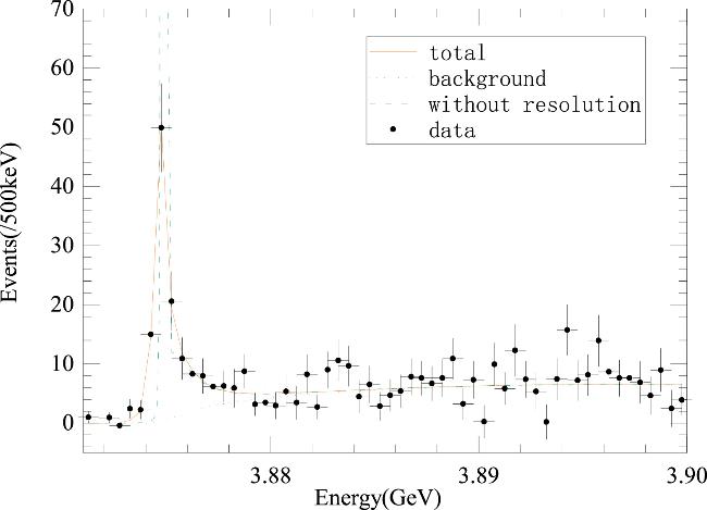
The Tcc state is so close to threshold (recalling the value of δmpole in equation (We use the optimization algorithm of MINUIT package to perform the minimization of χ2 [34]. The parameter values are shown in table 1. In the calculation, all the mass, energy and momentum are expressed in units of MeV. Then the units for the parameters are also given in the table. The fit result is shown in Figure 1, where ‘Energy’ corresponds to the invariant mass of D0D0π+. In fact, near the pole (signal) region, the invariant mass ${M}_{{D}^{* +}{D}^{0}}\approx {M}_{P}\approx {M}_{{D}^{0}{D}^{0}{\pi }^{+}}$. From the following discussions, we claim the Tcc state can be understood as the D*+D0 bound state. For a bound state case, the aforementioned ${ \mathcal N }\approx 1$ is clear since Lorentzian distribution reduces to a delta function. Yconst can then be understood as the yield corresponding to the product of production cross section of Tcc and branching fractions of Tcc → D*+D0 and D*+ → D0π+ (note that cross section has dimension of [MeV]−2).
Table 1. Our best values of the seven fitted parameters, with χ2 per degree of freedom being 0.93. |
| Yconst = (10.8 ± 8.0) MeV−2 | ||
| λ = (83.6 ± 63.8) MeV2 | β = (70.5 ± 37.6) MeV | MCDD − mth = (0.47 ± 0.38) MeV |
| a = − (81.4 ± 2.8) MeV−2 | b = − (99.2 ± 10.8) MeV−3 | c = (1653.5 ± 41.9) MeV−4 |
Figure 1. Mass spectrum for the D0D0π+ decay channel. The data are from the LHCb collaboration [2]. The solid line represents our total result, with the dotted line showing the background and the dashed line corresponding to without the Gaussian resolution. |
3. Scattering parameter, pole and compositeness
Using the central values of the fitted parameters, one obtains the scattering length a = 1.8 fm and the effective range r = − 77.2 fm. The value of r is so large that the effective range expansion method is not an appropriate tool in this case. Within uncertainties we have another set of parameter value, λ = 19.8, β = 108.0, MCDD = 0.47 + mth, which leads to a = − 3.0 fm, r = − 18.3 fm. The values of r are not the typical magnitude of a few fermi. So we will concentrate on the outcome of our CDD analysis.
The definition of compositeness for a bound state is well defined by the Weinberg formula [35, 36]. However, for resonance case, the compositeness calculated in that way will become a complex-valued number. As mentioned before, there are several developments for defining the compositeness. We will follow the one developed in [20] for a resonance18 ) corresponds to the physical value on the real axis, or GI(s + iε) in the physical sheet.
$\begin{eqnarray}X=| {\gamma }_{s}{| }^{2}{\left|\frac{dG(s)}{ds}\right|}_{s={E}_{P}^{2}},\end{eqnarray}$
for the case of $\sqrt{\,\rm{Re}\,{E}_{P}^{2}}$ larger than the lightest threshold for a coupled-channel scattering. $-{\gamma }_{s}^{2}$ is the residue of t(s) at the resonance pole position, ${E}_{P}^{2}$, of the complex s plane in the second RS $\begin{eqnarray}{t}^{\,\rm{II}\,}(s)\to \frac{-{\gamma }_{s}^{2}}{s-{E}_{P}^{2}}.\end{eqnarray}$
${\gamma }_{s}^{2}$ is related to γE by [26, 28] $\begin{eqnarray}{\gamma }_{s}^{2}=-16\pi {\gamma }_{E}{E}_{P}^{2}\times \frac{{E}_{P}-{M}_{\,\rm{CDD}\,}}{\lambda }.\end{eqnarray}$
G(s) is the two-point Green function, and the infinity can be removed by cutoff regularization or the dimensional regularization [37]. Its form in the dimensional regularization scheme at the regularization scale μ can be written as [30] $\begin{eqnarray}\begin{array}{rcl}G(s) & = & \alpha ({\mu }^{2})+\frac{1}{{(4\pi )}^{2}}\\ & & \times \left(\mathrm{log}\frac{{m}_{2}^{2}}{{\mu }^{2}}-{\varkappa }_{+}\mathrm{log}\frac{{\varkappa }_{+}-1}{{\varkappa }_{+}}-{\varkappa }_{-}\mathrm{log}\frac{{\varkappa }_{-}-1}{{\varkappa }_{-}}\right),\end{array}\end{eqnarray}$
with $\begin{eqnarray}\begin{array}{rcl}{\varkappa }_{\pm } & = & \frac{s+{m}_{1}^{2}-{m}_{2}^{2}}{2s}\pm \frac{p}{\sqrt{s}},\\ p & = & \frac{\sqrt{(s-{({m}_{1}-{m}_{2})}^{2})(s-{({m}_{1}+{m}_{2})}^{2})}}{2\sqrt{s}}.\end{array}\end{eqnarray}$
It is equivalent to the one used in [38]. The G(s) defined in equation (Resonance appears as a pole in the second RS. We thus need to make an analytical extrapolation of G(s) to the second RS. The result is given by 20 ) implies the condition of Im s > 0. For Im s < 0 case, using the Schwarz reflection principle G(s*) = [G(s)]*, one has 15 ) for a resonance. For a bound state (EB) case, one simply has 15 ) versus X = 0.232 from equation (23 ).
$\begin{eqnarray}\begin{array}{rcl}{G}^{\,\rm{II}\,}(s+{\rm{i}}\epsilon ) & = & {G}^{\,\rm{I}\,}(s+{\rm{i}}\epsilon )+\frac{{\rm{i}}}{4\pi \sqrt{s}}\\ & & \times \frac{\sqrt{(s-{({m}_{1}-{m}_{2})}^{2})(s-{({m}_{1}+{m}_{2})}^{2})}}{2\sqrt{s}}.\end{array}\end{eqnarray}$
The left and right side of equation ( $\begin{eqnarray}\begin{array}{rcl}{G}^{\,\rm{II}\,}(s-{\rm{i}}\epsilon ) & = & {G}^{\,\rm{I}\,}(s-{\rm{i}}\epsilon )-\frac{{\rm{i}}}{4\pi \sqrt{s}}\\ & & \times \frac{\sqrt{(s-{({m}_{1}-{m}_{2})}^{2})(s-{({m}_{1}+{m}_{2})}^{2})}}{2\sqrt{s}}.\end{array}\end{eqnarray}$
It is GII that should be used in equation ( $\begin{eqnarray}X=-{\gamma }_{s}^{2}{\left.\frac{d{G}^{\,\rm{I}\,}(s)}{ds}\right|}_{s={E}_{B}^{2}},\end{eqnarray}$
and of course γs is calculated in the physical sheet. The situation of X = 1 corresponds to a pure bound state or molecular. The elementariness Z = 1 − X measures the weight of all other components in the hadron wave function. In fact, the non-relativistic form of G(s) is $\frac{1}{8\pi {m}_{\,\rm{th}\,}}(\beta -{\rm{i}}k)$, and then to be consistent in the non-relativistic frame, one has $\begin{eqnarray}X=\frac{1}{8\pi {m}_{\,\rm{th}\,}}\left|\frac{\mu {\gamma }_{s}^{2}}{2{E}_{P}{k}_{P}}\right|,\end{eqnarray}$
with the pole momentum ${k}_{P}=\sqrt{2\mu ({E}_{P}-{m}_{\,\rm{th}\,})}$. In a real numerical calculation, such difference is negligible, for e.g. X = 0.232 deducing from equation (We search for the pole in the complex energy plane. We first consider the well-defined elastic scattering case with ${{\rm{\Gamma }}}_{{D}^{* +}}\to 0$. As a result, for the central value of the fitted parameter we find a pole 3874.72 MeV in the physical sheet, as a bound state; and a pole 3874.48 − i 1.74 MeV in the unphysical Riemann sheet, as a resonance. By slowly varying, e.g. the values of MCDD, both poles move gradually. For the bound state pole, we have the residue ${\gamma }_{s}^{2}=5.04$ GeV2, and the corresponding compositeness X = 0.23. Considering the uncertainties in table 1 within one sigma region, we have ${\gamma }_{s}^{2}=5.0{4}_{-1.60}^{+2.16}$ GeV2 and $X=0.2{3}_{-0.09}^{+0.40}$. As for the uncertainty, it is always hard to be quantified well. In the current calculation, we take the uncertainty from MIGRAD method in MINUIT subroutine. On the other hand, the propagation of the error for the parameter to the final X value is highly nonlinear, since we need to search for the corresponding pole and calculate its residue for each parameter set. We discretize the parameter values into dozen of sets and then get dozen of poles, residues, and X. Then the central value, upper value, lower value are extracted. The parameter set λ = 19.8, β = 33.0, MCDD = 0.47 in table 1 gives X = 0.63, which leads to the largest uncertainty. The LHCb collaboration uses the Weinberg compositeness formula involving the values of the scattering length and effective range, to investigate the elementariness Z value. The result is Z < 0.52 (0.58) at 90 (95)% confidence level. So it implies the compositeness X > 0.46 at 90% confidence level, which overlap with our value of X in some range. However, much work towards the detailed study of X still needs to be done.
The finite but small D*+ width moves the aforementioned resonance pole to 3874.5 − i1.73 MeV and the bound state pole to 3874.72 − i 0.0098 MeV. It is interesting to note that our such finding of a bound state pole agrees well with [39], where they find a bound state with width of 80keV by using the complex scaling method. Using the parameter values λ = 19.8, β = 108.0, MCDD = 0.47 + mth we can achieve a bound state pole at 3875.4 − i 0.039 with the width of 78 keV for the unstable bound state. If the condition $\sqrt{\,\rm{Re}\,\,{E}_{P}^{2}}\geqslant {m}_{\,\rm{th}\,}$ is fulfilled for a resonance pole, the compositeness formula, equation (15 ), could be applied and the compositeness X ranges from 0.07 to 0.57 accordingly. In fact, given that both poles appear in the physical and unphysical sheet, Tcc should rather be an elementary state, e.g. the compact tetraquark component takes a large or even dominant portion, according to the Morgan criterion [40].
For a fit, one usually worries the local minimum. We illustrate this briefly here. In [28], we have imposed a pole in the second sheet with pole parameters given by the experimental determination. In this way, λ and β are expressed as functions of MCDD, and then two parameters will be reduced. We have tried the similar exercise in our present study. The fit result is acceptable, but not as good as the one above. One of the reason could be that the width of Tcc is much narrower or the peak is more prominent than the ones for Zb states. We will not show its parameter value and figure. However, the conclusion that both poles in the first and second sheet are found does not change. In the second sheet, the pole is at −0.36 MeV + mth − i 0.024 MeV (cf. equation (1 )), as required. In this case, we cannot provide its compositeness value since it locates below the threshold. For the bound state case, a small compositeness number is found, which implies the compact tetraquark component in its wave function cannot be overlooked. That is, this fit solution does not influence our main conclusion at all. Certainly, we prefer the solution that is presented in the table 1 and figure 1.
4. Conclusion and outlook
The mystery of Tcc state reported by LHCb has not been unveiled, where various interpretations are proposed. We utilize an amplitude including the CDD pole to incorporate the nontrivial and non-perturbative final state interaction of D*+D0. This method provides much more information than the effective range expansion method. The appearing parameters are λ, β and MCDD, which will be fixed by fitting to the data. In the fit the experimental energy bin width and mass resolution function are considered. With the known parameters, we search for the pole in the complex energy plane. Both poles are found in the physical and unphysical Riemann sheet. This indicates that Tcc can be interpreted as an elementary state, e.g. the compact tetraquark component takes a large portion. The coupled-channel study following [26] may render more useful information and this work is ongoing.