


1. Introduction
The absence of significant deviations from the Standard Model (SM) at the Large Hadron Collider (LHC) up to the TeV scale suggests that the energy scale of new physics (NP) may lie well beyond the reach of current experiments, thereby making the direct detection of NP challenging. In this context, there has been considerable motivation in the indirect measurement of NP signals through low-energy experiments. Theoretically, hard NP corrections to low-energy theories can be systematically incorporated using the effective field theory (EFT) framework. In high-energy experiments above the electroweak scale, NP phenomena are effectively described by the standard model effective field theory (SMEFT) [1–8]. Simultaneously, there is growing interest in exploring NP through low-energy experiments below the electroweak scale. The physics of such processes is more accurately described by the low-energy effective field theory (LEFT), which encapsulates both electroweak-scale physics and NP effects through high-dimensional operators. The operator basis of LEFT has been the subject of extensive research. The complete sets of dimension-5 and dimension-6 operators of LEFT were first presented in [9], followed by the dimension-7 operators presented in [10]. Subsequently, [11] established the complete operator bases from dimension-5 to 9, leveraging the amplitude-operator correspondence [12]. These operators are constrained only by Lorentz and gauge symmetries, allowing them to describe a broad range of physics beyond the Standard Model at the electroweak scale. Consequently, precise determinations of the Wilson coefficients associated with LEFT operators can provide valuable constraints on potential NP models.
To provide precise predictions for experiments at different low-energy scales, the Wilson coefficients must be corrected for renormalization effects, which are governed by the renormalization group equations (RGEs). The complete RGEs for LEFT dimension-5 and dimension-6 operators have been calculated at the one-loop level in [13, 14]. Recently, efforts have also been made to extend these calculations to the two-loop level for dimension-5 operators [15]. Traditionally, the RGEs for Wilson coefficients are derived from the renormalization of off-shell Green’s functions. The complexity arises when matching the ultraviolet (UV) divergences to the operator basis, which requires the use of the equations of motion, and also when the gauge fields are involved. On the other hand, the advantages of the on-shell amplitude method have already been revealed in the literature, both in the construction of operator bases for EFTs [12, 16–18] and in loop-level amplitude calculations [19–21]. By placing external particles on-shell and retaining only physical polarizations, the equations of motion are automatically satisfied, and the gauge redundancy is eliminated. Notably, [22] established a connection between the renormalization scale dependence of operator form factors and their discontinuities by enforcing analyticity and unitarity. To date, the on-shell unitarity method has been extensively employed in the calculation of the anomalous dimensions [23–31].
In this work, we describe the development of the on-shell method combined with the unitarity cut for one-loop operator renormalization calculations. As an illustration, we compute the one-loop QCD contributions to the dimension-7 RGEs of LEFT, arising from dimension-7 operator mixing.
The paper is organized as follows. In section 2 , we provide a brief overview of LEFT, list the operators considered in this work, and define the RGEs and anomalous dimensions. Section 3 outlines the workflow of the on-shell unitarity method for deriving anomalous dimensions from the renormalization of form factors of LEFT operators, along with a shortcut for extracting the UV divergence from the rational part of the double-cut phase-space integrals. The results of the RGEs calculated in this work are presented in section 4 .
2. LEFT operators and anomalous dimensions
The gauge symmetry below the electroweak scale is spontaneously broken to SU(3)C × U(1)Q. Particles with masses at or above the electroweak scale, such as SM particles (W±, Z, the Higgs boson and the top quark), and NP particles become inactive and can be integrated out of the UV theory. The resulting LEFT Lagrangian can be written as [9]2.1 ), the QCD and QED Lagrangians are given by
$\begin{eqnarray}{{ \mathcal L }}_{\,\rm{LEFT}\,}={{ \mathcal L }}_{\,\rm{QCD+QED}\,}+{{ \mathcal L }}_{\mathrm{L\unicode{x00338}}}^{(3)}+\displaystyle \sum _{d\geqslant 5}\displaystyle \sum _{i}{L}_{i}^{(d)}{{ \mathcal O }}_{i}^{(d)}.\end{eqnarray}$
In ( $\begin{eqnarray}\begin{array}{rcl}{{ \mathcal L }}_{\,\rm{QCD+QED}\,} & = & -\frac{1}{4}{G}_{\mu \nu }^{A}{G}^{A\mu \nu }-\frac{1}{4}{F}_{\mu \nu }{F}^{\mu \nu }\\ & & +{\theta }_{\,\rm{QCD}\,}\frac{{g}^{2}}{32{\pi }^{2}}{G}_{\mu \nu }^{A}{\tilde{G}}^{A\mu \nu }+{\theta }_{\,\rm{QED}\,}\frac{{{\rm{e}}}^{2}}{32{\pi }^{2}}{F}_{\mu \nu }{\tilde{F}}^{\mu \nu }\\ & & +\displaystyle \sum _{\psi =u,d,{\rm{e}}}\left[\overline{\psi }{\rm{i}}\mathrm{D\unicode{x00338}}\psi -\left({\overline{\psi }}_{Rr}{M}_{\begin{array}{c}\psi \\ rs\end{array}}{\psi }_{Ls}+\,\rm{h.c.}\,\right)\right]\\ & & +{\overline{\nu }}_{L}{\rm{i}}\mathrm{\partial \unicode{x00338}}{\nu }_{L},\end{array}\end{eqnarray}$
where ${G}_{\mu \nu }^{A}$ and Fμν are the gluon and photon field strength tensors respectively, ${\tilde{G}}_{\mu \nu }={\epsilon }_{\mu \nu \rho \sigma }{G}^{\rho \sigma }/2$, where εμνρσ is the fourth-rank totally antisymmetric tensor with the convention ε0123 = + 1. The fermion fields consist of nu = 2 u-type quarks, nd = 3 d-type quarks, ne = 3 charged leptons, and nν = 3 left-handed neutrinos. The gauge covariant derivative is defined as ${D}_{\mu }={\partial }_{\mu }-{\rm{i}}{g}_{\,\rm{s}\,}{T}^{A}{G}_{\mu }^{A}-{\rm{i}}{\rm{e}}Q{A}_{\mu }$, where gs and e are the QCD and QED gauge coupling parameters respectively, and TA and Q are the color and the electric charge generators. r, s are flavor indices which take values in the range 1, …, nψ for each type of fermion. The Dirac mass matrix Mψ is allowed to mix different flavors within each fermion type. At the energy scale of LEFT, the QED contributions remain negligible while the QCD effects become predominant. When approaching the characteristic energy scale of QCD (ΛQCD ∼ 200 MeV), the strong coupling parameter ${\alpha }_{s}={g}_{s}^{2}/4\pi $ exhibits divergent behavior in the RGE of αs. For the calculation of operator anomalous dimensions, we exclusively consider the QCD particle interactions. The θ-terms in the Lagrangian, being total derivatives, do not contribute to the perturbative calculations of the RGEs or the scattering amplitudes of physical processes. These terms are included in the original paper [9] mainly to analyze the holomorphicity of the operator basis.The dimension-3 term in the Lagrangian is the Majorana mass term of left-handed neutrinos
$\begin{eqnarray}{{ \mathcal L }}_{\mathrm{L\unicode{x00338}}}^{(3)}=-\frac{1}{2}{M}_{\begin{array}{c}\nu \\ rs\end{array}}{\nu }_{Lr}^{{\rm{T}}}C{\nu }_{Ls}+\,\rm{h.c.}\,{,}\end{eqnarray}$
where C = iγ0γ2 is the charge conjugation matrix. The Majorana mass term violates the lepton number by ΔL = ± 2. In this work, we focus on the case where the baryon and the lepton numbers are conserved (ΔB = ΔL = 0) as an illustration. The calculation methods employed here can be straightforwardly extended to scenarios where baryon and lepton numbers are violated.The higher-dimensional terms of the LEFT Lagrangian are organized into operators ${{ \mathcal O }}_{i}^{(d)}$ multiplied by corresponding Wilson coefficients ${L}_{i}^{(d)}$. The superscript d denotes the mass dimension of each operator. The mass dimensions of the Wilson coefficients can be deduced through dimensional analysis of the Lagrangian, and they scale with the order of the electroweak scale v. Specifically, ${L}_{i}^{(d)}\sim 1/{v}^{d-4}$. The power counting in LEFT is governed by small ratios p/v and m/v, where p and m are momenta and masses of the particles in LEFT. A LEFT scattering amplitude with multiple insertions of higher-dimensional operators $\{{{ \mathcal O }}_{i}^{({d}_{i})}\}$ is suppressed by 1/vd−4 in the LEFT power counting with d defined by
$\begin{eqnarray}d-4=\displaystyle \sum _{i}\left({d}_{i}-4\right).\end{eqnarray}$
In this paper, we consider one-loop QCD corrections to the mixing among the LEFT dimension-7 operators. The operators considered in this work are listed in table 1 [10, 11], which contain only quark and gluon fields, and naturally conserve the baryon and lepton numbers. These results can be straightforwardly generalized to the baryon/lepton number violating operators, as well as to the one-loop QED correction. In general we will also need to take account of the multiple insertions of the dimension-6 and the dimension-5 operators to the one-loop renormalization of dimension-7 operators, which we will explore further in forthcoming work.
Table 1. Dimension-7 LEFT operators involving only the QCD degrees of freedom. The derivative operator is defined as $\overline{A}{\overleftrightarrow{D}}_{\mu }B\equiv \overline{A}{D}_{\mu }B-\overline{A}{\overleftarrow{D}}_{\mu }B$, where $\overline{A}{\overleftarrow{D}}_{\mu }={\partial }_{\mu }\overline{A}+\overline{A}{\rm{i}}{g}_{\,\rm{s}\,}{T}^{A}{G}_{\mu }^{A}$. |
| $\left(\overline{\,\rm{R}\,}\rm{L}\,\right){\,\rm{X}}^{2}\,+\,\,\rm{h.c.}\,$ | |
| ${{ \mathcal O }}_{\,\rm{uG1}\,}$ | $\left({\overline{u}}_{R}{u}_{L}\right){G}_{\mu \nu }^{A}{G}^{A\mu \nu }$ |
| ${{ \mathcal O }}_{\,\rm{uG2}\,}$ | $\left({\overline{u}}_{R}{u}_{L}\right){G}_{\mu \nu }^{A}{\widetilde{G}}^{A\mu \nu }$ |
| ${{ \mathcal O }}_{\,\rm{uG3}\,}$ | ${d}^{ABC}\left({\overline{u}}_{R}{T}^{A}{u}_{L}\right){G}_{\mu \nu }^{B}{G}^{C\mu \nu }$ |
| ${{ \mathcal O }}_{\,\rm{uG4}\,}$ | ${d}^{ABC}\left({\overline{u}}_{R}{T}^{A}{u}_{L}\right){G}_{\mu \nu }^{B}{\widetilde{G}}^{C\mu \nu }$ |
| ${{ \mathcal O }}_{\,\rm{uG5}\,}$ | ${f}^{ABC}\left({\overline{u}}_{R}{\sigma }^{\mu \nu }{T}^{A}{u}_{L}\right){G}_{\mu \rho }^{B}{G}_{\nu }^{C\rho }$ |
| ${{ \mathcal O }}_{\,\rm{dG1}\,}$ | $\left({\overline{d}}_{R}{d}_{L}\right){G}_{\mu \nu }^{A}{G}^{A\mu \nu }$ |
| ${{ \mathcal O }}_{\,\rm{dG2}\,}$ | $\left({\overline{d}}_{R}{d}_{L}\right){G}_{\mu \nu }^{A}{\widetilde{G}}^{A\mu \nu }$ |
| ${{ \mathcal O }}_{\,\rm{dG3}\,}$ | ${d}^{ABC}\left({\overline{d}}_{R}{T}^{A}{d}_{L}\right){G}_{\mu \nu }^{B}{G}^{C\mu \nu }$ |
| ${{ \mathcal O }}_{\,\rm{dG4}\,}$ | ${d}^{ABC}\left({\overline{d}}_{R}{T}^{A}{d}_{L}\right){G}_{\mu \nu }^{B}{\widetilde{G}}^{C\mu \nu }$ |
| ${{ \mathcal O }}_{\,\rm{dG5}\,}$ | ${f}^{ABC}\left({\overline{d}}_{R}{\sigma }^{\mu \nu }{T}^{A}{d}_{L}\right){G}_{\mu \rho }^{B}{G}_{\nu }^{C\rho }$ |
| | |
| $\left(\overline{\,\rm{L}\,}\,\rm{L}\,\right)\left(\overline{\,\rm{L}\,}\,\rm{R}\,\right)\,+\,\,\rm{h.c.}\,$ | |
| | |
| ${{ \mathcal O }}_{\,\rm{uuD1}\,}$ | $\left({\overline{u}}_{L}{\gamma }^{\mu }{u}_{L}\right)\left({\overline{u}}_{L}{\rm{i}}\overleftrightarrow{{D}_{\mu }}{u}_{R}\right)$ |
| ${{ \mathcal O }}_{\,\rm{ddD1}\,}$ | $\left({\overline{d}}_{L}{\gamma }^{\mu }{d}_{L}\right)\left({\overline{d}}_{L}{\rm{i}}\overleftrightarrow{{D}_{\mu }}{d}_{R}\right)$ |
| ${{ \mathcal O }}_{\,\rm{udD1}\,}$ | $\left({\overline{u}}_{L}{\gamma }^{\mu }{u}_{L}\right)\left({\overline{d}}_{L}{\rm{i}}\overleftrightarrow{{D}_{\mu }}{d}_{R}\right)$ |
| ${{ \mathcal O }}_{\,\rm{udD2}\,}$ | $\left({\overline{u}}_{L}{\gamma }^{\mu }{T}^{A}{u}_{L}\right)\left({\overline{d}}_{L}{T}^{A}{\rm{i}}\overleftrightarrow{{D}_{\mu }}{d}_{R}\right)$ |
| ${{ \mathcal O }}_{\,\rm{duD1}\,}$ | $\left({\overline{d}}_{L}{\gamma }^{\mu }{d}_{L}\right)\left({\overline{u}}_{L}{\rm{i}}\overleftrightarrow{{D}_{\mu }}{u}_{R}\right)$ |
| ${{ \mathcal O }}_{\,\rm{duD2}\,}$ | $\left({\overline{d}}_{L}{\gamma }^{\mu }{T}^{A}{d}_{L}\right)\left({\overline{u}}_{L}{T}^{A}{\rm{i}}\overleftrightarrow{{D}_{\mu }}{u}_{R}\right)$ |
| | |
| $\left(\overline{\,\rm{R}\,}\,\rm{R}\,\right)\left(\overline{\,\rm{L}\,}\rm{R}\,\right)+\,\rm{h.c.}$ | |
| | |
| ${{ \mathcal O }}_{\,\rm{uuD2}\,}$ | $\left({\overline{u}}_{R}{\gamma }^{\mu }{u}_{R}\right)\left({\overline{u}}_{L}{\rm{i}}\overleftrightarrow{{D}_{\mu }}{u}_{R}\right)$ |
| ${{ \mathcal O }}_{\,\rm{ddD2}\,}$ | $\left({\overline{d}}_{R}{\gamma }^{\mu }{d}_{R}\right)\left({\overline{d}}_{L}{\rm{i}}\overleftrightarrow{{D}_{\mu }}{d}_{R}\right)$ |
| ${{ \mathcal O }}_{\,\rm{udD3}\,}$ | $\left({\overline{u}}_{R}{\gamma }^{\mu }{u}_{R}\right)\left({\overline{d}}_{L}{\rm{i}}\overleftrightarrow{{D}_{\mu }}{d}_{R}\right)$ |
| ${{ \mathcal O }}_{\,\rm{udD4}\,}$ | $\left({\overline{u}}_{R}{\gamma }^{\mu }{T}^{A}{u}_{R}\right)\left({\overline{d}}_{L}{T}^{A}{\rm{i}}\overleftrightarrow{{D}_{\mu }}{d}_{R}\right)$ |
| ${{ \mathcal O }}_{\,\rm{duD3}\,}$ | $\left({\overline{d}}_{R}{\gamma }^{\mu }{d}_{R}\right)\left({\overline{u}}_{L}{\rm{i}}\overleftrightarrow{{D}_{\mu }}{u}_{R}\right)$ |
| ${{ \mathcal O }}_{\,\rm{duD4}\,}$ | $\left({\overline{d}}_{R}{\gamma }^{\mu }{T}^{A}{d}_{R}\right)\left({\overline{u}}_{L}{T}^{A}{\rm{i}}\overleftrightarrow{{D}_{\mu }}{u}_{R}\right)$ |
Perturbative corrections to the LEFT amplitude introduce UV divergences. Technically, these divergences are handled by dimensional regularization (DR) which analytically continues the spacetime dimension to D = 4 − 2ε. The divergences can be subsequently canceled by the $\overline{\,\rm{MS}\,}$ counter-terms of the Wilson coefficients by adjusting the bare coefficient
$\begin{eqnarray}{L}_{i,0}={S}_{\epsilon }^{-{r}_{i}}{\mu }^{2{r}_{i}\epsilon }\left[{L}_{i}(\mu )+\delta {L}_{i}(\mu )\right],\end{eqnarray}$
where ${S}_{\epsilon }={\left(4\pi \right)}^{\epsilon }{{\rm{e}}}^{-\epsilon {\gamma }_{\,\rm{E}\,}}$ is a factor defined by the $\overline{\,\rm{MS}\,}$ scheme, δLi(μ) is the counter-term and Li(μ) is the renormalized Wilson coefficient, 2riε accounts for the fractional dimension of the bare coefficient in dimensional regularization (for example αs,0, ri = 1), which deviates from its four-dimensional counterpart. Note that hereinafter we omit the superscripts for dimension-7 operators and Wilson coefficients for simplicity. The renormalization scale μ can be chosen to be some typical scale of the low-energy process under study, so that the counter-terms cancel the UV divergence in loop integrals without producing large logarithms. The bare coefficient Li,0 is a renormalization scale independent. The μ dependence of the renormalized Wilson coefficients is described by the renormalization group equations (RGEs) $\begin{eqnarray}\frac{{\rm{d}}{L}_{i}\left(\mu \right)}{{\rm{d}}\,{\mathrm{ln}}\,\mu }=-2{r}_{i}\epsilon {L}_{i}\left(\mu \right)+{\gamma }_{ij}{L}_{j}(\mu )\,+\,\cdots ,\end{eqnarray}$
where γij are the anomalous dimensions originated from the mixing effects among the dimension-7 operators. The ellipsis represents the nonlinear terms of the Wilson coefficients from dimension-5 and 6 not considered in this paper. We will obtain the values of γij in the subsequent sections.3. Obtaining anomalous dimensions from on-shell form factors
The anomalous dimensions of the operators can be extracted from the renormalization of the corresponding form factors. The form factors associated with the LEFT operators are defined as
$\begin{eqnarray}\begin{array}{l}{{ \mathcal F }}_{i,n}\left({p}_{1},\ldots ,\,\,{p}_{n}\right)\\ \quad \equiv \displaystyle \int {{\rm{d}}}^{D}x\,{{\rm{e}}}^{-{\rm{i}}q\cdot x}{\,}_{{\rm{out}}}\langle {p}_{1},\ldots ,\,\,{p}_{n}| {{ \mathcal O }}_{i}\left(x\right)| 0{\rangle }_{\,\rm{in}\,},\end{array}\end{eqnarray}$
where pa are the momenta of outgoing particles which are chosen to align with the types of fields in the operator ${{ \mathcal O }}_{i}$, q = ∑apa is the momentum flowing into ${{ \mathcal O }}_{i}$.At loop levels, the form factor ${{ \mathcal F }}_{i,n}$ is plagued by both UV and infrared (IR)ll divergences. The UV divergence is canceled by the counter-terms in LEFT along with the multiplicative renormalization factor Zij for ${{ \mathcal O }}_{i}$. The IR divergence can also be written as a universal multiplicative factor ZIR which is a matrix in the color space of external particles [32–34]. Consequently, one can define the finite form factors as
$\begin{eqnarray}{\widetilde{{ \mathcal F }}}_{j,n}\left(\mu \right)={{\boldsymbol{Z}}}_{\,\rm{IR}\,}^{-1}\left(\mu \right){{ \mathcal F }}_{i,n}{Z}_{ij}\left(\mu \right).\end{eqnarray}$
Only Zij is relevant to the operator anomalous dimension and it is insensitive to IR scales. So for simplicity we treat quark propagators as massless and treat their mass terms as interactions. At a one-loop level, the universal IR factor takes the form
$\begin{eqnarray}\begin{array}{rcl}{{\boldsymbol{Z}}}_{\,\rm{IR}\,}^{-1} & = & 1-\left[\frac{{\alpha }_{\,\rm{s}\,}}{4\pi }\displaystyle \sum _{1\leqslant a\lt b\leqslant n}{{\boldsymbol{T}}}_{a}\cdot {{\boldsymbol{T}}}_{b}\right.\\ & & \left.\times \left(\frac{1}{{\epsilon }^{2}}+\frac{1}{\epsilon }\,{\mathrm{ln}}\,\frac{{\mu }^{2}}{-{s}_{ab}}\right)+\displaystyle \sum _{1\leqslant a\leqslant n}\frac{{\gamma }_{\,\rm{coll}\,}^{a}}{2\epsilon }\right],\end{array}\end{eqnarray}$
where ${s}_{ab}\equiv {\left({p}_{a}+{p}_{b}\right)}^{2}$, ${\gamma }_{\,\rm{coll}\,}^{a}$ are the so-called collinear anomalous dimensions for quarks and gluons $\begin{eqnarray}{\gamma }_{\,\rm{coll}\,}^{q}=-\left(\frac{{\alpha }_{\rm{s}\,}}{4\pi }\right)3{C}_{\,\rm{F}},\end{eqnarray}$
$\begin{eqnarray}{\gamma }_{\,\rm{coll}\,}^{g}=-\left(\frac{{\alpha }_{\rm{s}}}{4\pi }\right){b}_{0}.\end{eqnarray}$
Ta is the color generator associated with the a-th external particle and ${{\boldsymbol{T}}}_{a}\cdot {{\boldsymbol{T}}}_{b}\equiv {{\boldsymbol{T}}}_{a}^{A}{{\boldsymbol{T}}}_{b}^{A}$. For QCD with N colors and nf = nu + nd flavors, ${C}_{\,\rm{F}\,}=\left({N}^{2}-1\right)/\left(2N\right)$, CA = N and ${T}_{\rm{F}\,}=1/2.{b}_{0}=\frac{11}{3}{C}_{\rm{A}}-\frac{4}{3}{T}_{\,\rm{F}}{n}_{f}$ is the one-loop beta function of the strong coupling.
We are only interested in the non-total-derivative operators in the LEFT Lagrangian. After the IR divergence has been extracted, We take q → 0 for the remaining UV divergent terms to derive Zij, which automatically removes contributions from total-derivative operators.
Taking the total derivative of (3.2 ) with respect to μ, we get the Callan–Symanzik equation, which describes how the μ scaling of a form factor is related to the explicit ${\mathrm{ln}}\,\mu $ dependence in the expression and the implicit μ dependence of the renormalized parameters2.6 ) and is the aim of this work.
$\begin{eqnarray}\begin{array}{rcl}\mu \frac{{\rm{d}}}{{\rm{d}}\mu }{\widetilde{{ \mathcal F }}}_{j,n}\left(\mu \right) & = & \left(\mu \frac{\partial }{\partial \mu }+{\beta }_{g}\frac{\partial }{\partial g}+{\beta }_{i}\frac{\partial }{\partial {L}_{i}}\right)\\ & & \times {\widetilde{{ \mathcal F }}}_{j,n}\left(\mu \right)+{ \mathcal O }\left(\epsilon \right)\\ & = & \left({\delta }_{ij}{{\boldsymbol{\gamma }}}_{\,\rm{IR}\,}-{\gamma }_{ij}\right){\widetilde{{ \mathcal F }}}_{i,n}\left(\mu \right),\end{array}\end{eqnarray}$
where g represents the QCD and QED coupling parameters gs and e. The IR anomalous dimension γIR takes the form $\begin{eqnarray}\begin{array}{rcl}{{\boldsymbol{\gamma }}}_{\,\rm{IR}\,} & = & -{{\boldsymbol{Z}}}_{\,\rm{IR}\,}^{-1}\frac{{\rm{d}}{{\boldsymbol{Z}}}_{\,\rm{IR}\,}}{{\rm{d}}\,{\mathrm{ln}}\,\mu }=\left(\frac{{\alpha }_{\,\rm{s}\,}}{4\pi }\right)\\ & & \times \displaystyle \sum _{1\leqslant a\lt b\leqslant n}2{{\boldsymbol{T}}}_{a}\cdot {{\boldsymbol{T}}}_{b}\,{\mathrm{ln}}\,\frac{{\mu }^{2}}{-{s}_{ab}}+\displaystyle \sum _{1\leqslant a\leqslant n}{\gamma }_{\,\rm{coll}\,}^{a}.\end{array}\end{eqnarray}$
The UV anomalous dimension takes the form $\begin{eqnarray}{\gamma }_{ij}\equiv -{\mu }^{-2\left({r}_{i}-{r}_{j}\right)\epsilon }{Z}_{ik}^{-1}\frac{{\rm{d}}{Z}_{kj}}{{\rm{d}}\,{\mathrm{ln}}\,\mu },\end{eqnarray}$
which can be shown to be identical to the quantity introduced in (Instead of evaluating directly from the renormalization factor Zij, the UV anomalous dimension γij can also be derived directly from the Callan–Symanzik equation (3.5 ). To accomplish this, [22, 35, 36] finds a substitute to evaluate the partial derivative of μ in (3.5 ). We give a short explanation building upon [24, 37].
After factoring out the Lorentz structures, the scalar functions of ${{ \mathcal F }}_{i,n}$ only depend on the dimensionless ratios sab/μ2 with sab > 0. Therefore the partial derivative of μ applied to these parts can be traded for the dilatation operator
$\begin{eqnarray}-\mu \frac{\partial }{\partial \mu }\to {\rm{D}}\equiv \displaystyle \sum _{a}{p}_{a}^{\mu }\frac{\partial }{\partial {p}_{a}^{\mu }},\end{eqnarray}$
The application of the dilatation operator to the form factors gives $\begin{eqnarray}\begin{array}{l}{{\rm{e}}}^{{\rm{i}}\left(\pi -0\right){\rm{D}}}{{ \mathcal F }}_{i,n}\left({p}_{1},\ldots ,\,{p}_{n}\right)\\ \quad =\displaystyle \int {{\rm{d}}}^{D}x\,{{\rm{e}}}^{-{\rm{i}}q\cdot x}{\,}_{\,\rm{in}\,}{\langle {p}_{1},\ldots ,\,{p}_{n}{{ \mathcal O }}_{i}\left(x\right)| 0\rangle }_{\,\rm{in}\,}\\ \quad =\displaystyle \sum _{X}{\,}_{\,\rm{in}\,}{\langle {p}_{1},\ldots ,\,{p}_{n}| X\rangle }_{\,\rm{out}\,}\displaystyle \int {{\rm{d}}}^{D}x\,{{\rm{e}}}^{-{\rm{i}}q\cdot x}{\,}_{\,\rm{out}\,}{\langle X| {{ \mathcal O }}_{i}\left(x\right)| 0\rangle }_{\,\rm{in}\,}\\ \quad =\displaystyle \sum _{X}{{ \mathcal S }}_{n,X}^{\dagger }{{ \mathcal F }}_{i,X},\end{array}\end{eqnarray}$
where the S-matrix is given by ${{ \mathcal S }}_{ab}={\delta }_{ab}+{\rm{i}}{{ \mathcal A }}_{ab}$. Expanding the exponential of D with respect to perturbative orders and using the Callan–Symanzik equation, we find a relation between anomalous dimensions and the cut diagrams of the form factors. For minimal form factors of ${{ \mathcal O }}_{j}$ that do not involve a coupling constant at tree level, we find the one-loop formula: $\begin{eqnarray}\begin{array}{l}{\rm{D}}{\widetilde{{ \mathcal F }}}_{j,n}^{\{1\}}\left(\mu \right)=\left({\gamma }_{ij}^{\{1\}}-{\delta }_{ij}{{\boldsymbol{\gamma }}}_{\,\rm{IR}\,}^{\{1\}}\right){\widetilde{{ \mathcal F }}}_{i,n}^{\{0\}}\\ \quad =\,-\frac{1}{\pi }\displaystyle \sum _{X}{{ \mathcal A }}_{X,n}^{\{0\}}{\widetilde{{ \mathcal F }}}_{j,X}^{\{0\}}-\left[{\rm{D}}{\left({{\boldsymbol{Z}}}_{\,\rm{IR}\,}^{-1}\right)}^{\{1\}}\right]{\widetilde{{ \mathcal F }}}_{j,n}^{\{0\}},\end{array}\end{eqnarray}$
where we use {k} to represent perturbative orders which is distinguished from the power counting (d). The last term appears because ZIR depends explicitly on ${\mathrm{ln}}\,\mu $. Note that the UV renormalization factor Zij has no explicit dependence on ${\mathrm{ln}}\,\mu $ when written in terms of renormalized parameters, so there is no such term for it.At a one-loop level, the summation of X in (3.10 ) contains a two-body phase-space integration, which we express in terms of spinor helicity formalism [38–41], (as it simplifies the structure of amplitudes and form factors): 3.11 ) can be interpreted as double cuts in the one-loop form factor [44, 45]. For triangle and box integrals, the cut integrand always have single poles of $\bar{z}$, which is evaluated to logarithms under the $\bar{z}$ integral. So by separating the $\bar{z}$ integral with respect to the rational and logarithmic terms 3.20 ) gives the master formula for evaluating the anomalous dimensions in this work. One can verify that in (3.20 ), only tree amplitudes are required, which is a considerable simplification compared to the direct calculation of one-loop amplitudes. The tree amplitudes for renormalizable gauge theories are well-known and can be constructed via on-shell recursion, such as the Britto-Cachazo-Feng-Witten (BCFW) recursion formula [46, 47]. While the application of on-shell recursion to EFTs faces certain challenges [48], this is not an issue for us, as only contact EFT amplitudes are needed for the present work.
$\begin{eqnarray}\begin{array}{l}\displaystyle \sum _{X}{{ \mathcal A }}_{X,n}^{\{0\}}{\widetilde{{ \mathcal F }}}_{j,X}^{\{0\}}\\ \quad =\displaystyle \int {\rm{d}}{{\rm{\Pi }}}_{2}\displaystyle \sum _{\begin{array}{c}X\,\rm{types}\,\,\,\rm{helicity}\,\end{array}}{{ \mathcal A }}_{X,n}^{\{0\}}\left(| l\rangle ,| l]\right){{ \mathcal F }}_{j,X}^{\{0\}}\left(| -l\rangle ,| -l]\right).\end{array}\end{eqnarray}$
We apply the parameterization of [42] to write the two-body phase-space measure as $\begin{eqnarray}\begin{array}{rcl}{\rm{d}}{{\rm{\Pi }}}_{2} & = & {\displaystyle \int }_{\langle \lambda {| }^{\ast }=| \lambda ]}\frac{[\lambda \,{\rm{d}}\lambda ]\wedge \langle {\rm{d}}\lambda \,\lambda \rangle }{16{\rm{i}}{\pi }^{2}[\lambda | K| \lambda \rangle }\\ & & \times \displaystyle \int {\rm{d}}t\,t\,{\delta }^{(+)}\left(t-\frac{{K}^{2}}{[\lambda | K| \lambda \rangle }\right),\end{array}\end{eqnarray}$
where K is the total momentum that flows through the cut, and $\begin{eqnarray}| l\rangle =\sqrt{t}| \lambda \rangle ,\quad | l]=\sqrt{t}| \lambda ].\end{eqnarray}$
We choose two reference massless momenta P, Q satisfying the relation $\begin{eqnarray}K=P+Q,\end{eqnarray}$
then λ can be decomposed into $\begin{eqnarray}| \lambda \rangle =| P\rangle +z| Q\rangle ,\quad | \lambda ]=| P]+\bar{z}| Q]\end{eqnarray}$
with two independent parameters $z,\bar{z}$. After this change of variables, the phase space measure is written as $\begin{eqnarray}\begin{array}{rcl}{\rm{d}}{{\rm{\Pi }}}_{2} & = & \frac{1}{16{\rm{i}}{\pi }^{2}}\mathop{\displaystyle \int }\limits_{{z}^{* }=\bar{z}}{\rm{d}}\bar{z}\wedge {\rm{d}}z\\ & & \times \displaystyle \int {\rm{d}}t\,{t}^{2}\,{\delta }^{(+)}\left(t-\frac{1}{1+z\bar{z}}\right),\end{array}\end{eqnarray}$
where the z* denotes the complex conjugate of z. The integral over t can be trivially evaluated. In order to perform the integrals of $z,\bar{z}$, we adopt the generalized Cauchy formula [21]: $\begin{eqnarray}{\int }_{{z}^{\ast }=\bar{z}}{\rm{d}}\bar{z}\wedge {\rm{d}}z\to -\oint {\rm{d}}z\int {\rm{d}}\bar{z}.\end{eqnarray}$
As a check, the plain integral of the two-body phase-space gives $\begin{eqnarray}\begin{array}{rcl}{{\rm{\Pi }}}_{2} & = & \displaystyle \int {\rm{d}}{{\rm{\Pi }}}_{2}=\frac{-1}{16{\rm{i}}{\pi }^{2}}\oint {\rm{d}}z\\ & & \times \displaystyle \int {\rm{d}}\bar{z}\frac{1}{{\left(1+z\bar{z}\right)}^{2}}=\frac{1}{8\pi }.\end{array}\end{eqnarray}$
The one-loop form factor can be regarded as a linear combination of the scalar integrals in the PV reduction [43]. The bubble integrals contain all the UV divergences as well as the collinear divergences that contributes to the collinear anomalous dimensions. Triangle and box integrals contain only IR divergences which contribute to the logarithmic part of the IR anomalous dimensions, which are irrelevant to our calculation. The phase-space integral ( $\begin{eqnarray}\begin{array}{l}\displaystyle \int \frac{{\rm{d}}\bar{z}}{{\left(1+z\bar{z}\right)}^{2}}\displaystyle \sum _{\begin{array}{c}X\,\rm{types}\,\,\,\rm{helicity}\,\end{array}}{{ \mathcal A }}_{X,n}^{\{0\}}\left(z,\bar{z}\right){{ \mathcal F }}_{j,X}^{\{0\}}\left(z,\bar{z}\right)\\ \quad \equiv F\left(z,\bar{z}\right)={F}^{\,\rm{rat}\,}\left(z,\bar{z}\right)+{F}^{\,{\rm{log}}\,}\left(z,\bar{z}\right),\end{array}\end{eqnarray}$
one can extract the bubble integral contribution directly from Frat [21]: $\begin{eqnarray}\begin{array}{rcl}\mu \frac{\partial }{\partial \mu }{\left.{\widetilde{{ \mathcal F }}}_{j,n}^{\{1\}}\right|}_{\,\rm{bubbles}\,} & = & \left({\delta }_{ij}\displaystyle \sum _{a}{\gamma }_{\,\rm{coll}\,}^{a\{1\}}-{\gamma }_{ij}^{\{1\}}\right){\widetilde{{ \mathcal F }}}_{i,n}^{\{0\}}\\ & = & \frac{1}{\pi }{\left(\displaystyle \int {\rm{d}}{{\rm{\Pi }}}_{2}\displaystyle \sum _{\begin{array}{c}X\,\rm{types}\,\,\,\rm{helicity}\,\end{array}}{{ \mathcal A }}_{X,n}^{\{0\}}{{ \mathcal F }}_{j,X}^{\{0\}}\right)}^{\,\rm{rat}\,},\end{array}\end{eqnarray}$
where we have dropped the contributions due to logarithmic terms of IR anomalous dimensions. (4. Anomalous dimensions of dimension-7 operators
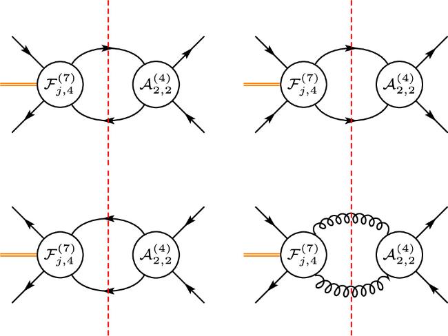
Figure 1. Double-cut diagrams for the on-shell one-loop form factors of dimension-7 $q\bar{q}q\bar{q}$ form factors. |
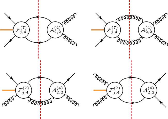
Figure 2. Double-cut diagrams for the on-shell one-loop form factors of dimension-7 $q\bar{q}gg$ form factors. |
As an illustration, we present a detailed calculation of the one-loop anomalous dimensions for the Wilson coefficients ${L}_{\begin{array}{c}\,\rm{uuD1}\,\\ prst\end{array}}$arising from the contributions of ${L}_{\begin{array}{c}\,\rm{duD}\,i\end{array}}$. Taking the 12∣34 cut as an example, the required dimension-4 amplitudes for constructing the double-cut diagrams are given by
$\begin{eqnarray}\begin{array}{rcl}{{ \mathcal A }}^{(4)}\left({\left({l}_{1}\right)}_{d},{\left({l}_{2}\right)}_{\bar{d}};{3}_{u},{4}_{\bar{u}}\right) & = & 2{g}_{\,\rm{s}\,}^{2}{({T}^{A})}^{{i}_{3}}{\,}_{{i}_{4}}{({T}^{A})}^{{i}_{6}}{\,}_{{i}_{5}}{\delta }^{st}{\delta }^{uv}{A}^{(4)}\\ & & \times \left({\left({l}_{1}\right)}_{d},{\left({l}_{2}\right)}_{\bar{d}};{3}_{u},{4}_{\bar{u}}\right)\end{array}\end{eqnarray}$
with $\begin{eqnarray}{A}^{(4)}\left({\left({l}_{1}\right)}_{d}^{+},{\left({l}_{2}\right)}_{\bar{d}}^{-};{3}_{u}^{+},{4}_{\bar{u}}^{-}\right)=\frac{[{l}_{1}\,3]\langle {l}_{2}\,4\rangle }{{s}_{34}},\end{eqnarray}$
$\begin{eqnarray}{A}^{(4)}\left({\left({l}_{1}\right)}_{d}^{+},{\left({l}_{2}\right)}_{\bar{d}}^{-};{3}_{u}^{-},{4}_{\bar{u}}^{+}\right)=\frac{[{l}_{1}\,4]\langle {l}_{2}\,3\rangle }{{s}_{34}},\end{eqnarray}$
$\begin{eqnarray}{A}^{(4)}\left({\left({l}_{1}\right)}_{d}^{-},{\left({l}_{2}\right)}_{\bar{d}}^{+};{3}_{u}^{+},{4}_{\bar{u}}^{-}\right)=\frac{\langle {l}_{1}\,4\rangle [{l}_{2}\,3]}{{s}_{34}},\end{eqnarray}$
$\begin{eqnarray}{A}^{(4)}\left({\left({l}_{1}\right)}_{d}^{-},{\left({l}_{2}\right)}_{\bar{d}}^{+};{3}_{u}^{-},{4}_{\bar{u}}^{+}\right)=\frac{\langle {l}_{1}\,3\rangle [{l}_{2}\,4]}{{s}_{34}},\end{eqnarray}$
where l1, l2 are incoming and p3, p4 are outgoing momenta, while all helicities follow the outgoing convention. ∣ − l⟩ = − ∣l⟩, ∣ − l] = ∣l]. The dimension-7 tree-level form factors can be decomposed with respect to the color structures:
$\begin{eqnarray}\begin{array}{rcl}{{ \mathcal F }}_{j}^{(7)}\left({1}_{u},{2}_{\bar{u}},{\left({l}_{1}\right)}_{d},{\left({l}_{2}\right)}_{\bar{d}}\right) & = & {({T}^{A})}^{{i}_{1}}{\,}_{{i}_{2}}{({T}^{A})}^{{i}_{5}}{\,}_{{i}_{6}}{F}_{j,4}^{(7)[8]}\\ & & +{\delta }_{{i}_{2}}^{{i}_{1}}{\delta }_{{i}_{6}}^{{i}_{5}}{F}_{j,4}^{(7)[1]},\end{array}\end{eqnarray}$
where only the color octet part contributes after the contraction with ${{ \mathcal A }}_{2,2}^{(4)}$. All non-zero values of ${F}_{j,4}^{(7)[8]}$ are listed below, $\begin{eqnarray}\begin{array}{l}{F}_{\begin{array}{c}\,\rm{duD2}\,\\ xyzw\end{array}}^{(7)[8]}\left({1}_{u}^{+},{2}_{\bar{u}}^{+};{\left({l}_{1}\right)}_{d}^{+},{\left({l}_{2}\right)}_{\bar{d}}^{-}\right)\\ \quad ={\delta }^{xu}{\delta }^{yv}{\delta }^{zp}{\delta }^{wr}[1\,2][{l}_{1}| {p}_{2}-{p}_{1}| {l}_{2}\rangle ,\end{array}\end{eqnarray}$
$\begin{eqnarray}\begin{array}{l}{F}_{\begin{array}{c}\,\rm{duD4}\,\\ xyzw\end{array}}^{(7)[8]}\left({1}_{u}^{+},{2}_{\bar{u}}^{+};{\left({l}_{1}\right)}_{d}^{-},{\left({l}_{2}\right)}_{\bar{d}}^{+}\right)\\ \quad ={\delta }^{xu}{\delta }^{yv}{\delta }^{zp}{\delta }^{wr}[1\,2][{l}_{2}| {p}_{2}-{p}_{1}| {l}_{1}\rangle ,\end{array}\end{eqnarray}$
$\begin{eqnarray}\begin{array}{l}{F}_{\begin{array}{c}{\,\rm{duD2}\,}^{* }\\ xyzw\end{array}}^{(7)[8]}\left({1}_{u}^{-},{2}_{\bar{u}}^{-};{\left({l}_{1}\right)}_{d}^{+},{\left({l}_{2}\right)}_{\bar{d}}^{-}\right)\\ \quad ={\delta }^{xv}{\delta }^{yu}{\delta }^{zr}{\delta }^{wp}\langle 1\,2\rangle [{l}_{1}| {p}_{2}-{p}_{1}| {l}_{2}\rangle ,\end{array}\end{eqnarray}$
$\begin{eqnarray}\begin{array}{l}{F}_{\begin{array}{c}{\,\rm{duD4}\,}^{* }\\ xyzw\end{array}}^{(7)[8]}\left({1}_{u}^{-},{2}_{\bar{u}}^{-};{\left({l}_{1}\right)}_{d}^{-},{\left({l}_{2}\right)}_{\bar{d}}^{+}\right)\\ \quad ={\delta }^{xv}{\delta }^{yu}{\delta }^{zr}{\delta }^{wp}\langle 1\,2\rangle [{l}_{2}| {p}_{2}-{p}_{1}| {l}_{1}\rangle .\end{array}\end{eqnarray}$
By applying the momentum conservation condition l2 = p1 + p2 − l1, and parameterizing l1 using (3.13 ) and (3.15 ) 3.20 ) by employing the generalized Cauchy formula.
$\begin{eqnarray}| {l}_{1}\rangle =\sqrt{t}\left(| 1\rangle +z| 2\rangle \right),\quad \langle {l}_{1}| =\sqrt{t}\left(\langle 1| +z\langle 2| \right),\end{eqnarray}$
$\begin{eqnarray}| {l}_{1}]=\sqrt{t}\left(| 1]+\bar{z}| 2]\right),\quad [{l}_{1}| =\sqrt{t}\left([1| +\bar{z}[2| \right).\end{eqnarray}$
Considering the helicity configuration $\left({1}_{u}^{+},{2}_{\bar{u}}^{+},{3}_{u}^{+},{4}_{\bar{u}}^{-}\right)$, we can get $\begin{eqnarray}\begin{array}{l}{F}_{\begin{array}{c}\,\rm{duD2}\,\\ xyzw\end{array}}^{(7)[8]}\left({1}_{u}^{+},{2}_{\bar{u}}^{+},{\left({l}_{1}\right)}_{d}^{+},{\left({l}_{2}\right)}_{\bar{d}}^{-}\right)\\ \quad \times {A}^{(4)}\left({\left({l}_{1}\right)}_{d}^{-},{\left({l}_{2}\right)}_{\bar{d}}^{+};{3}_{u}^{+},{4}_{\bar{u}}^{-}\right)\\ \quad =-2{T}_{\rm{F}\,}{g}_{\,\rm{s}}^{2}{({T}^{A})}^{{i}_{3}}{\,}_{{i}_{4}}{({T}^{A})}^{{i}_{1}}{\,}_{{i}_{2}}\\ \quad \times {\delta }^{st}{\delta }^{xy}{\delta }^{zp}{\delta }^{wr}\frac{[1\,{l}_{1}]\langle {l}_{1}\,4\rangle \langle 1\,{l}_{2}\rangle [{l}_{2}\,3]}{\langle 1\,2\rangle }\\ \quad =-2{T}_{\rm{F}\,}{g}_{\,\rm{s}}^{2}{({T}^{A})}^{{i}_{3}}{\,}_{{i}_{4}}{({T}^{A})}^{{i}_{1}}{\,}_{{i}_{2}}{\delta }^{st}{\delta }^{xy}{\delta }^{zp}{\delta }^{wr}\\ \quad \times [1\,2][1\,3]\langle 1\,4\rangle {t}^{2}{w}_{1}\bar{z}{({\bar{w}}_{2}z+1)}^{2},\end{array}\end{eqnarray}$
where we define $\begin{eqnarray}\begin{array}{rcl}{w}_{1} & = & \frac{[2\,3]}{[1\,3]}=-\frac{\langle 1\,4\rangle }{\langle 2\,4\rangle },\quad {\bar{w}}_{1}=\frac{\langle 2\,3\rangle }{\langle 1\,3\rangle }=-\frac{[1\,4]}{[2\,4]},\\ {w}_{2} & = & \frac{[2\,4]}{[1\,4]}=-\frac{\langle 1\,3\rangle }{\langle 2\,3\rangle },\quad {\bar{w}}_{2}=\frac{\langle 2\,4\rangle }{\langle 1\,4\rangle }=-\frac{[1\,3]}{[2\,3]}.\end{array}\end{eqnarray}$
where ${w}_{1}{\bar{w}}_{2}={w}_{2}{\bar{w}}_{1}=-1,{w}_{1}{\bar{w}}_{1}={s}_{14}/{s}_{13},{w}_{2}{\bar{w}}_{2}={s}_{13}/{s}_{14}$. The poles of the integrand are shown in figure 3. Throughout the calculation, we consistently eliminate l1 and l2 using the form ⟨m li⟩[n li]. For example, $\begin{eqnarray}\begin{array}{rcl}\langle 1\,{l}_{2}\rangle [{l}_{2}\,3] & = & \langle 1| {p}_{1}+{p}_{2}-{l}_{1}| 3]\\ & = & \langle 1\,2\rangle [2\,3]-\langle 1\,{l}_{1}\rangle [{l}_{1}\,3]\\ & = & \langle 1\,2\rangle [2\,3]\left(1-\frac{z\bar{z}-{\bar{w}}_{2}z}{1+z\bar{z}}\right)\\ & = & \langle 1\,2\rangle [2\,3]\frac{{\bar{w}}_{2}z+1}{1+z\bar{z}}\\ & = & \langle 1\,2\rangle [2\,3]t({\bar{w}}_{2}z+1).\end{array}\end{eqnarray}$
We express t in terms of $1/(1+z\bar{z})$, and vice versa. All integrands share the general form $\begin{eqnarray*}\begin{array}{l}[\,\rm{Color}\,]\cdot [\,\rm{Flavor}\,]\cdot [\,\rm{Kinematic}\,]\\ \quad \cdot [\,\rm{dimensionless function of}\,(t,{w}_{i}\bar{z},{\bar{w}}_{i}z)].\end{array}\end{eqnarray*}$
We perform the phase-space integral in (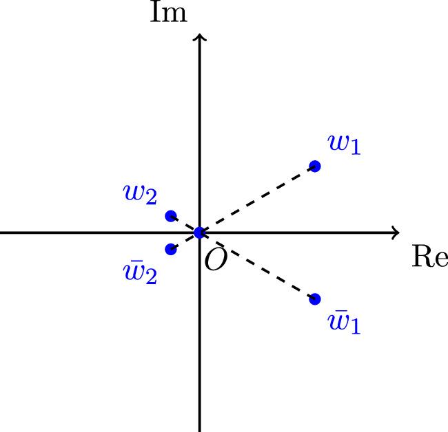
Figure 3. The points on the complex plane denote the poles of the integrand,where w1, w2 are the corresponding poles associated with z, ${\bar{w}}_{1},{\bar{w}}_{2}$ are the corresponding poles associated with $\bar{z}$, 0 is both for $z,\bar{z}$. |
After summing all the double-cut contributions, the result becomes 3.20 ), which correspond to the coefficients in the RGE: 4.13 ).
$\begin{eqnarray*}\begin{array}{l}\frac{1}{\pi }{\left(\displaystyle \int {\rm{d}}{{\rm{\Pi }}}_{2}\displaystyle \sum _{\begin{array}{c}\,\rm{double cuts}\,\,\,\rm{helicity}\,\end{array}}{{ \mathcal A }}_{2,2}^{(4)}{{ \mathcal F }}_{j,4}^{(7)}\right)}^{\,\rm{rat}\,}\\ \quad =\frac{-1}{8{\pi }^{2}}\frac{4{g}_{\rm{s}\,}^{2}{T}_{\,\rm{F}}^{2}}{3}\left({\delta }_{{i}_{4}}^{{i}_{1}}{\delta }_{{i}_{2}}^{{i}_{3}}-\frac{1}{{N}_{\,\rm{c}\,}}{\delta }_{{i}_{2}}^{{i}_{1}}{\delta }_{{i}_{4}}^{{i}_{3}}\right){\delta }^{st}{\delta }^{xy}{\delta }^{zp}{\delta }^{wr}\\ \quad \times [1\,2][1\,3]\langle 1\,4\rangle -\left(1,p\right)\leftrightarrow \left(3,s\right),\\ \quad j=\rm{duD2}\,{,}\,\rm{duD 4}.\end{array}\end{eqnarray*}$
In comparison with $\begin{eqnarray}\begin{array}{rcl}{{ \mathcal F }}_{\begin{array}{c}\,\rm{uuD1}\,\\ xyzw\end{array}}^{(7)} & = & 2{\delta }_{{i}_{2}}^{{i}_{1}}{\delta }_{{i}_{4}}^{{i}_{3}}{\delta }^{xs}{\delta }^{yt}{\delta }^{zp}{\delta }^{wr}[1\,2][1\,3]\\ & & \times \langle 1\,4\rangle -\left(1,p\right)\leftrightarrow \left(3,s\right),\end{array}\end{eqnarray}$
one can deduce the anomalous dimensions ${\gamma }_{ij}^{\{1\}}$ from ( $\begin{eqnarray}\begin{array}{rcl}{\dot{L}}_{\begin{array}{c}\,\rm{uuD1}\,\\ stpr\end{array}} & = & -\frac{4{g}_{\rm{s}\,}^{2}{T}_{\,\rm{F}}^{2}}{3}\left[\frac{1}{{N}_{\,\rm{c}\,}}{\delta }^{st}\left({L}_{\begin{array}{c}\rm{duD2}\,\\ wwpr\end{array}}+{L}_{\begin{array}{c}\,\rm{duD4}\\ wwpr\end{array}}\right)\right.\\ & & \left.+{\delta }^{pt}\left({L}_{\begin{array}{c}\rm{duD2}\,\\ wwsr\end{array}}+{L}_{\begin{array}{c}\,\rm{duD4}\\ wwsr\end{array}}\right)\right]+\cdots \,.\end{array}\end{eqnarray}$
The full result of ${\dot{L}}_{\,\rm{uuD1}\,}$ is listed in (The anomalous dimensions are written in terms of the RGEs of the dimension-7 Wilson coefficients. We adopt the notation from [49] to define
$\begin{eqnarray}\dot{L}\equiv 16{\pi }^{2}\mu \frac{{\rm{d}}L}{{\rm{d}}\mu }.\end{eqnarray}$
The RGEs are given by
$\begin{eqnarray}\begin{array}{rcl}{\dot{L}}_{\begin{array}{c}\,\rm{uuD1}\,\\ prst\end{array}} & = & \frac{{N}_{\rm{c}\,}^{2}-1}{{N}_{\rm{c}}}{g}_{\rm{s}}^{2}{L}_{\begin{array}{c}\rm{uuD1}\\ prst\end{array}}+\frac{1}{3}{\delta }^{pr}\frac{1}{{N}_{\rm{c}}}{g}_{\,\rm{s}}^{2}\\ & & \times \left(2{L}_{\begin{array}{c}\rm{uuD1}\,\\ swwt\end{array}}+2{L}_{\begin{array}{c}\rm{uuD2}\\ wtsw\end{array}}-{L}_{\begin{array}{c}\rm{duD2}\\ wwst\end{array}}-{L}_{\begin{array}{c}\,\rm{duD4}\\ wwst\end{array}}\right)\\ & & +\frac{1}{3}{\delta }^{rs}{g}_{\,\rm{s}\,}^{2}\left(2{L}_{\begin{array}{c}\,\rm{uuD1}\,\\ pwwt\end{array}}\right.\\ & & \left.+2{L}_{\begin{array}{c}\rm{uuD2}\,\\ wtpw\end{array}}-{L}_{\begin{array}{c}\rm{duD2}\\ wwpt\end{array}}-{L}_{\begin{array}{c}\,\rm{duD4}\\ wwpt\end{array}}\right),\end{array}\end{eqnarray}$
$\begin{eqnarray}\begin{array}{rcl}{\dot{L}}_{\begin{array}{c}\,\rm{uuD2}\,\\ prst\end{array}} & = & \frac{{N}_{\rm{c}\,}^{2}-1}{{N}_{\rm{c}}}{g}_{\rm{s}}^{2}{L}_{\begin{array}{c}\rm{uuD2}\\ prst\end{array}}+\frac{1}{3}{\delta }^{pr}\frac{1}{{N}_{\rm{c}}}{g}_{\,\rm{s}}^{2}\\ & & \times \left(2{L}_{\begin{array}{c}\rm{uuD1}\,\\ swwt\end{array}}+2{L}_{\begin{array}{c}\rm{uuD2}\\ wtsw\end{array}}-{L}_{\begin{array}{c}\rm{duD2}\\ wwst\end{array}}-{L}_{\begin{array}{c}\,\rm{duD4}\\ wwst\end{array}}\right)\\ & & +\frac{1}{3}{\delta }^{pt}{g}_{\,\rm{s}\,}^{2}\left(2{L}_{\begin{array}{c}\,\rm{uuD1}\,\\ swwr\end{array}}\right.\\ & & \left.+2{L}_{\begin{array}{c}\rm{uuD2}\,\\ wrsw\end{array}}-{L}_{\begin{array}{c}\rm{duD2}\\ wwsr\end{array}}-{L}_{\begin{array}{c}\,\rm{duD4}\\ wwsr\end{array}}\right),\end{array}\end{eqnarray}$
$\begin{eqnarray}{\dot{L}}_{\begin{array}{c}\,\rm{ddD}\,i\\ prst\end{array}}={\left.{\dot{L}}_{\begin{array}{c}\,\rm{uuD}\,i\\ prst\end{array}}\right|}_{u\leftrightarrow d},\,\end{eqnarray}$
$\begin{eqnarray}{\dot{L}}_{\begin{array}{c}\rm{udD1}\,\\ prst\end{array}}=\frac{{N}_{\rm{c}}^{2}-1}{{N}_{\rm{c}}}{g}_{\rm{s}}^{2}{L}_{\begin{array}{c}\,\rm{udD1}\\ prst\end{array}},\,\end{eqnarray}$
$\begin{eqnarray}\begin{array}{rcl}{\dot{L}}_{\begin{array}{c}\,\rm{udD2}\,\\ prst\end{array}} & = & \frac{{N}_{\rm{c}\,}^{2}-1}{{N}_{\rm{c}}}{g}_{\rm{s}}^{2}{L}_{\begin{array}{c}\rm{udD2}\\ prst\end{array}}+\frac{2}{3}{\delta }^{pr}{g}_{\,\rm{s}}^{2}\\ & & \times \left({L}_{\begin{array}{c}\rm{udD2}\,\\ wwst\end{array}}+{L}_{\begin{array}{c}\rm{udD4}\\ wwst\end{array}}-2{L}_{\begin{array}{c}\rm{ddD1}\\ swwt\end{array}}-2{L}_{\begin{array}{c}\,\rm{ddD2}\\ wtsw\end{array}}\right),\end{array}\end{eqnarray}$
$\begin{eqnarray}{\dot{L}}_{\begin{array}{c}\rm{udD3}\,\\ prst\end{array}}=\frac{{N}_{\rm{c}}^{2}-1}{{N}_{\rm{c}}}{g}_{\rm{s}}^{2}{L}_{\begin{array}{c}\,\rm{udD3}\\ prst\end{array}},\,\end{eqnarray}$
$\begin{eqnarray}\begin{array}{rcl}{\dot{L}}_{\begin{array}{c}\,\rm{udD4}\,\\ prst\end{array}} & = & \frac{{N}_{\rm{c}\,}^{2}-1}{{N}_{\rm{c}}}{g}_{\rm{s}}^{2}{L}_{\begin{array}{c}\rm{udD4}\\ prst\end{array}}+\frac{2}{3}{\delta }^{pr}{g}_{\,\rm{s}}^{2}\\ & & \times \left({L}_{\begin{array}{c}\rm{udD2}\,\\ wwst\end{array}}+{L}_{\begin{array}{c}\rm{udD4}\\ wwst\end{array}}-2{L}_{\begin{array}{c}\rm{ddD1}\\ swwt\end{array}}-2{L}_{\begin{array}{c}\,\rm{ddD2}\\ wtsw\end{array}}\right),\end{array}\end{eqnarray}$
$\begin{eqnarray}{\dot{L}}_{\begin{array}{c}\,\rm{duD}\,i\\ prst\end{array}}={\left.{\dot{L}}_{\begin{array}{c}\,\rm{udD}\,i\\ prst\end{array}}\right|}_{u\leftrightarrow d},\,\end{eqnarray}$
$\begin{eqnarray}\begin{array}{lcl}{\dot{L}}_{\begin{array}{c}\,\rm{uG1}\,\\ pr\end{array}} & = & \frac{1}{3{N}_{\rm{c}\,}}{g}_{\,\rm{s}}^{2}\left\{\Space{0ex}{3.25ex}{0ex}\left[4{N}_{\,\rm{c}\,}\left({n}_{u}+{n}_{d}\right)\right.\right.\\ & & \left.\left.-31{N}_{\rm{c}\,}^{2}+13\right]{L}_{\begin{array}{c}\,\rm{uG1}\\ pr\end{array}}-4{\rm{i}}{L}_{\begin{array}{c}\,\rm{uG2}\,\\ pr\end{array}}\right\}\\ & & +\frac{2\left({N}_{\rm{c}\,}^{2}-4\right)}{3{N}_{\rm{c}}^{2}}{g}_{\,\rm{s}}^{2}\left({L}_{\begin{array}{c}\,\rm{uG3}\,\\ pr\end{array}}-{\rm{i}}{L}_{\begin{array}{c}\rm{uG4}\,\\ pr\end{array}}\right)-6{g}_{\rm{s}}^{2}{L}_{\begin{array}{c}\,\rm{uG5}\\ pr\end{array}},\end{array}\end{eqnarray}$
$\begin{eqnarray}\begin{array}{lcl}{\dot{L}}_{\begin{array}{c}\,\rm{uG2}\,\\ pr\end{array}} & = & \frac{1}{3{N}_{\rm{c}\,}}{g}_{\,\rm{s}}^{2}\left\{4{\rm{i}}{L}_{\begin{array}{c}\,\rm{uG1}\,\\ pr\end{array}}\right.\\ & & \left.+\left[4{N}_{\,\rm{c}\,}\left({n}_{u}+{n}_{d}\right)-31{N}_{\rm{c}\,}^{2}+13\right]{L}_{\begin{array}{c}\,\rm{uG2}\\ pr\end{array}}\right\}\\ & & +\frac{2\left({N}_{\rm{c}\,}^{2}-4\right)}{3{N}_{\rm{c}}^{2}}{g}_{\,\rm{s}}^{2}\left({\rm{i}}{L}_{\begin{array}{c}\rm{uG3}\,\\ pr\end{array}}+{L}_{\begin{array}{c}\,\rm{uG4}\\ pr\end{array}}\right)+6{\rm{i}}{g}_{\rm{s}\,}^{2}{L}_{\begin{array}{c}\,\rm{uG5}\\ pr\end{array}},\end{array}\end{eqnarray}$
$\begin{eqnarray}\begin{array}{lcl}{\dot{L}}_{\begin{array}{c}\,\rm{uG3}\,\\ pr\end{array}} & = & {g}_{\,\rm{s}\,}^{2}\left\{\frac{4}{3}\left({L}_{\begin{array}{c}\,\rm{uG1}\,\\ pr\end{array}}-{\rm{i}}{L}_{\begin{array}{c}\,\rm{uG2}\,\\ pr\end{array}}\right)\right.\\ & & +\frac{1}{3{N}_{\,\rm{c}\,}}\left[4{N}_{\,\rm{c}\,}\left({n}_{u}+{n}_{d}\right)-8{N}_{\rm{c}\,}^{2}+1\right]{L}_{\begin{array}{c}\,\rm{uG3}\\ pr\end{array}}\\ & & \left.+\frac{{\rm{i}}\left({N}_{\rm{c}\,}^{2}+8\right)}{3{N}_{\rm{c}}}{L}_{\begin{array}{c}\rm{uG4}\\ pr\end{array}}-2{N}_{\rm{c}}{L}_{\begin{array}{c}\,\rm{uG5}\\ pr\end{array}}\right\},\end{array}\,\end{eqnarray}$
$\begin{eqnarray}\begin{array}{lcl}{\dot{L}}_{\begin{array}{c}\,\rm{uG4}\,\\ pr\end{array}} & = & {g}_{\,\rm{s}\,}^{2}\left\{\frac{4}{3}\left({\rm{i}}{L}_{\begin{array}{c}\rm{uG1}\,\\ pr\end{array}}+{L}_{\begin{array}{c}\,\rm{uG2}\\ pr\end{array}}\right)-\frac{{\rm{i}}\left({N}_{\rm{c}\,}^{2}+8\right)}{3{N}_{\rm{c}}}{L}_{\begin{array}{c}\,\rm{uG3}\\ pr\end{array}}\right.\\ & & +\frac{1}{3{N}_{\,\rm{c}\,}}\left[4{N}_{\,\rm{c}\,}\left({n}_{u}+{n}_{d}\right)-8{N}_{\,\rm{c}\,}^{2}+1\right]\\ & & \left.\times {L}_{\begin{array}{c}\,\rm{uG4}\,\\ pr\end{array}}+2{\rm{i}}{N}_{\rm{c}\,}{L}_{\begin{array}{c}\,\rm{uG5}\\ pr\end{array}}\right\},\end{array}\,\end{eqnarray}$
$\begin{eqnarray}\begin{array}{rcl}{\dot{L}}_{\begin{array}{c}\,\rm{uG5}\,\\ pr\end{array}} & = & -{g}_{\,\rm{s}\,}^{2}\left\{12\left({L}_{\begin{array}{c}\,\rm{uG1}\,\\ pr\end{array}}+{\rm{i}}{L}_{\begin{array}{c}\,\rm{uG2}\,\\ pr\end{array}}\right)\right.\\ & & +\frac{2\left({N}_{\rm{c}\,}^{2}-4\right)}{{N}_{\,\rm{c}}}\left({L}_{\begin{array}{c}\,\rm{uG3}\,\\ pr\end{array}}+{\rm{i}}{L}_{\begin{array}{c}\,\rm{uG4}\,\\ pr\end{array}}\right)\\ & & \left.+\frac{1}{3{N}_{\,\rm{c}\,}}\left[-4{N}_{\,\rm{c}\,}\left({n}_{u}+{n}_{d}\right)+{N}_{\rm{c}\,}^{2}+3\right]{L}_{\begin{array}{c}\,\rm{uG5}\\ pr\end{array}}\right\},\end{array}\end{eqnarray}$
$\begin{eqnarray}{\dot{L}}_{\begin{array}{c}\,\rm{dG}\,i\\ pr\end{array}}={\left.{\dot{L}}_{\begin{array}{c}\,\rm{uG}\,i\\ pr\end{array}}\right|}_{u\leftrightarrow d}.\,\end{eqnarray}$
Note that the results above are not complete. We also need the contributions of multiple dimension-5 and 6 Wilson coefficient terms, which is postponed to a subsequent work.
5. Conclusions
In this work, we investigated the application of the on-shell unitarity method to calculate the anomalous dimensions of dimension-7 operators in the LEFT. Compared to the traditional Feynman diagram approach, the on-shell method significantly simplifies the generation and simplification of scattering amplitudes. By utilizing a shortcut to extract the UV divergences from the rational terms in the phase-space integrals of the double-cut amplitudes, we circumvent the need for direct computation of loop integrals, thereby further reducing the complexity of the calculations. We derived the one-loop QCD corrections to the RGEs for the Wilson coefficients associated with the operator mixing among the dimension-7 operators in the LEFT. These results are instrumental in fitting the Wilson coefficients to experimental data across a range of energy scales. A complete set of dimension-7 RGEs should also incorporate contributions from the nonlinear terms of the dimension-5 and the dimension-6 Wilson coefficients. Additionally, due to the mass terms in the LEFT, the RGEs for Wilson coefficients associated with the operators of dimension less than 7 also receive corrections at dimension-7 order. We plan to address these contributions in a forthcoming publication.