


1. Introduction
The direct detection [1] of gravitational waves (GWs) by the Laser Interferometer Gravitational-Wave Observatory (LIGO) [2] has offered a novel method for exploring the physics of the early Universe [3–6]. GWs produced by axions or axion-like particles (ALPs), especially the stochastic gravitational wave background (SGWB) from the early Universe, enable the detection of new physics beyond the Standard Model and provide insights into the early Universe [7–14]. Axions were originally introduced to address the strong CP problem within the Standard Model [15–20]. While numerous mechanisms exist for the production of axions in the early Universe [21, 22], enabling a wide range of dark matter axion masses, these mechanisms may also contribute to various cosmological phenomena [23].
Axions and ALPs typically have weak couplings to photons or other Standard Model particles, making them difficult to detect directly [24, 25]. Moreover, these particles have been proposed to address other Standard Model and cosmological challenges, such as resolving the electroweak hierarchy problem [26, 27], serving as dark matter (DM) candidates [24, 28, 29] or inflatons [30], and being present in string theory frameworks [31]. The audible axions model proposed in [32, 33] describes the coupling between axions and dark photons (gauge bosons), in which dark photons experience tachyonic instability when axions oscillate. The model postulates that axions or ALPs possess large initial velocities, enabling the generation of detectable GW signals even with small decay constants. This process results in the generation of an SGWB in the early Universe, allowing us to detect these particles, which carry chirality. Parity violation will serve as a powerful observable for distinguishing cosmological background GWs from astrophysical ones [34]. Probing axion dark matter through future space-based gravitational-wave detectors will enable the exploration of broader parameter space for axions and ALPs. Except for the ground-based gravitational-wave observatories [35, 36], forthcoming space-based missions hold the potential to probe axion-like dark matter directly [37–39].
The SGWB arises from the superposition of GWs produced by a large number of independent sources [40]. It exhibits stochasticity and has a signal strength that is relatively weak compared to the total intensity sensitivity of detectors, categorizing it as a weak signal, and methods for its detection have been developed [41]. Due to the stochastic and uncorrelated nature of the general generation process, the SGWB is assumed to be unpolarized. However, parity violation in gravity, such as the Chern–Simons coupling [42, 43] and the Nieh–Yan coupling in teleparallel equivalent of general relativity (TEGR) [44–52], can modify the generation and propagation of gravitational waves, leading to a circularly polarized SGWB. The chirality of GWs can be effectively measured by several detectors, including ground-based interferometers [53–55]. While current ground-based detectors are insufficiently sensitive to constrain circular polarization significantly [56, 57], more precise measurements are expected in the coming years [58]. For space-based detection, the LISA-Taiji network [59–61] offers a promising approach due to its non-coplanar configuration. Additionally, Cosmic Microwave Background (CMB) observations [62, 63] provide an independent probe of circular polarization through primordial B-mode signatures.
LISA (Laser Interferometer Space Antenna) is a triangular GW detector in the orbit around the Sun, which is expected to be launched in the 2030s, with an arm length of L = 2.5 × 10⁹m [64]. Taiji is similar to LISA but has an arm length of L = 3 × 10⁹m [65]. Due to their planar configuration, individual detectors are insensitive to the chiral signatures of GWs. For an isotropic SGWB, the detection of its circular polarization requires the correlation of two non-coplanar gravitational wave detectors [66]. Therefore, a network of detectors is necessary, such as ground-based networks [67, 68] or the space-based network LISA-Taiji [61, 69–76], which can enhance the detection of the circular polarization of the SGWB. Furthermore, space-based GW detector networks also provide numerous other advantages, including improved gravitational wave polarization measurements [77], enhanced parameter estimation for Galactic binaries [78], better sky localization accuracy [79, 80], more accurate localization of massive binaries [81], detection of black hole formation mechanisms [82], increased detection capabilities for stellar binary black holes [83], and increased precision of GW standard sirens and cosmological parameter estimation [84–86].
To evaluate the detection capability of the LISA-Taiji network for chiral gravitational wave background (GWB), we estimate the spectral parameters and normalized model parameters of the chiral GWB generated by early cosmic axions using the Fisher information matrix. Additionally, we perform a Fisher analysis based on the fitted SGWB energy density spectrum from the dark photon coupling model [87] and broken power-law spectrum from the Nieh–Yan coupling model [52].
The paper is organized as follows. In section 2 , we briefly introduce how axions generate chiral gravitational waves through coupling with dark photons or the Nieh-–term, and present the energy density spectrum of the resulting gravitational waves, along with fitted templates and parameters. In section 3 , we describe the configuration of the space-based GW detector network and calculate its response to GWs. In section 4 , we derive the Fisher information matrix and determine the parameters for two different GW energy spectra with the network. In section 5 , we present the conclusion and discussion. The calculations in this work are performed using the Python packages numpy and scipy , and the plots are generated using matplotlib and GetDist .
2. Audible axions and chiral GW background
Several mechanisms that produce chiral GWs from audible axions have been explored in prior research. One is the coupling of axion to dark photon [32, 87, 88], while the other involves axion coupling to the parity-violating gravity such as Chern–Simons [89–91] and Nieh–Yan modified gravity [44–52]. The former just generates chiral GWs mediated by dark photons, while the latter can produce GWs directly and efficiently. In this section, we explore the GW spectrum template and fitting parameters produced by these mechanisms.
2.1. Chiral GWB from dark photon coupling
The chiral GWB can be generated through the asymmetrical production of dark photons [32, 87, 88]. In this mechanism, the total action can be expressed as
$\begin{aligned} S_{\mathrm{DP}}= & \int \mathrm{d}^{4} x \sqrt{-g}\left[\frac{M_{p}^{2}}{2} R-\frac{1}{4} X_{\mu \nu} X^{\mu \nu}+\frac{\alpha_{X}}{4 f_{X}} \phi X_{\mu \nu} \widetilde{X}^{\mu \nu}\right. \\ & \left.-\frac{1}{2} \partial_{\mu} \phi \partial^{\mu} \phi-V(\phi)\right] . \end{aligned}$
Here, fX is the decay constant of the axion, αX is the coupling coefficient and $V(\phi )={m}^{2}{f}_{X}^{2}\left[1-\cos \left(\frac{\phi }{{f}_{X}}\right)\right]$ is the cosine-like potential with the axion mass m. The third term in this action leads to a nontrivial dispersion relation for the helicities of dark photons, which takes the form ${\omega }_{X,\pm }^{2}={k}_{X}^{2}\mp {k}_{X}\frac{{\alpha }_{X}}{{f}_{X}}{\phi }^{{\prime} }$. This indicates that the asymmetric production of dark photons results in an oscillating stress-energy distribution that sources gravitational waves.Previous studies provide a well-fitting curve for the chiral gravitational wave energy density spectrum produced by dark photons. For the SGWB template, a suitable ansatz is [87]
$\begin{eqnarray}{\tilde{{\rm{\Omega }}}}_{{\rm{GW}}}({\tilde{f}}_{p})=\frac{{{ \mathcal A }}_{s}{\left({\tilde{f}}_{p}/{f}_{s}\right)}^{p}}{1+{\left({\tilde{f}}_{p}/{f}_{s}\right)}^{p}\exp \left[\gamma ({\tilde{f}}_{p}/{f}_{s}-1)\right]},\end{eqnarray}$
where ${\tilde{{\rm{\Omega }}}}_{{\rm{GW}}}\equiv {{\rm{\Omega }}}_{{\rm{GW}}}(f)/{{\rm{\Omega }}}_{{\rm{GW}}}({f}_{p})$ represents the normalized GW energy density, fp denotes the peak frequency. f denotes the GW frequency and ${\tilde{f}}_{p}\equiv f/{f}_{p}$ is the dimensionless normalized frequency. Moreover, ${{ \mathcal A }}_{s}$, fs, γ, p are the fitting parameters.From the derivation in [32], the peak amplitude and peak frequency of the GW spectrum, at the time of GW emission, are given by ${f}_{p}\simeq {({\alpha }_{X}\theta )}^{2/3}m,\,{{\rm{\Omega }}}_{{\rm{GW}}}({f}_{p})\simeq {\left(\frac{{f}_{X}}{{M}_{P}}\right)}^{4}\,{\left(\frac{{\theta }^{2}}{{\alpha }_{X}}\right)}^{\frac{4}{3}}\,$. Here, θ is the initial misalignment angle and MP ≃ 2.4 × 10¹⁸ GeV is the reduced Planck mass. Considering the expansion of the Universe, which leads to redshifting, these quantities become [32]
$\begin{eqnarray}{f}_{p}^{0}\simeq {({\alpha }_{X}\theta )}^{2/3}\,{T}_{0}{\left(\frac{{g}_{s,0}}{{g}_{s,* }}\right)}^{1/3}{\left(\frac{m}{{M}_{P}}\right)}^{1/2}\,,\end{eqnarray}$
$\begin{eqnarray}{{\rm{\Omega }}}_{{\rm{GW}}}^{0}({f}_{p}^{0})\simeq 1.67\times 1{0}^{-4}{g}_{s,* }^{-1/3}{\left(\frac{{f}_{X}}{{M}_{P}}\right)}^{4}\,{\left(\frac{{\theta }^{2}}{{\alpha }_{X}}\right)}^{\frac{4}{3}}.\end{eqnarray}$
Here, we choose the effective number of relativistic degrees of freedom gs,* = 106.75, because the mechanism occurs near the QCD phase transition. gs,0 = 3.938 is the effective relativistic degree of freedom today when the temperature T0 = 2.35 × 10⁻¹³ GeV. Based on the equations above, to produce detectable GW signals within the mHz frequency band, we adopt the following parameter values: m = 1.0 × 10⁻² eV, fX = 1.0 × 10¹⁷ GeV, αX = 55, and θ = 1.2, as proposed by [32].2.2. Chiral GWB from Nieh–Yan coupling
The chiral GWB can also be generated through an axion-like mechanism that couples to the Nieh–Yan term, resulting in the direct and efficient production of chiral GWB during the radiation-dominated epoch [52]. This generation arises from the tachyonic instability of gravitational perturbations induced by the Nieh–Yan term. The total action for this mechanism can be written as 1 ), fT is the axion decay constant, αT is the coupling coefficient and V(φ) represents the cosine-like potential. The second term in equation (5 ) can also lead to a nontrivial dispersion relation for the GW helicities, given by ${\omega }_{T,\pm }^{2}={k}_{T}^{2}\pm \frac{{\alpha }_{T}{\phi }^{{\prime} }}{{f}_{T}{M}_{P}^{2}}{k}_{T}$. The kT here is the wave vector for GWs, indicating that the last term produces an effect analogous to the term $\frac{{\alpha }_{X}}{4{f}_{X}}\phi {X}_{\mu \nu }{\widetilde{X}}^{\mu \nu }$ in the dark photon case.
$\begin{aligned} S_{\mathrm{NY}}= & \int \mathrm{d}^{4} x \sqrt{-g}\left[-\frac{M_{\mathrm{p}}^{2}}{2} \hat{T}+\frac{\alpha_{T} M_{\mathrm{p}}^{2}}{4 f_{T}} \phi \hat{T}_{A \mu \nu} \widetilde{T}^{A \mu \nu}\right. \\ & \left.-\frac{1}{2} \partial_{\mu} \phi \partial^{\mu} \phi-V(\phi)\right] . \end{aligned}$
Here, $\hat{T}$ is the torsion scalar, which is dynamically equivalent to the Ricci scalar in general relativity. Similar to the action in equation (Specifically, when the axion field oscillates, one of the GW helicities will have a range of modes with imaginary frequencies, resulting in a tachyonic instability that drives exponential growth. Since the growth rate is related to helicities, the left-handed and right-handed GWs are generated asymmetrically, ultimately leading to chiral GWB. In [52], the broken power-law template provides a better fit for the GW spectrum in this model, which can be written as
$\begin{eqnarray}{\tilde{{\rm{\Omega }}}}_{T}={\left({\tilde{f}}_{c}\right)}^{{\alpha }_{1}}{\left[1+0.75{\left({\tilde{f}}_{c}\right)}^{{\rm{\Delta }}}\right]}^{\frac{({\alpha }_{2}-{\alpha }_{1})}{{\rm{\Delta }}}}.\end{eqnarray}$
Here, ${\tilde{{\rm{\Omega }}}}_{T}\equiv {{\rm{\Omega }}}_{T}(f)/{{\rm{\Omega }}}_{c}$, where Ωc is the characteristic energy density. ${\tilde{f}}_{c}\equiv f/{f}_{c}$ is the dimensionless normalized frequency with the characteristic frequency fc. Moreover, α1, α2 and Δ are fitting parameters.In this equation, the characteristic frequency today, ${f}_{c}^{0}$, can be expressed in terms of physical parameters as
$\begin{eqnarray}{f}_{c}^{0}=0.7125\,\rm{mHz}\,{\left(\frac{100}{{g}_{s,* }}\right)}^{\frac{1}{12}}{\left(\frac{9}{14}{\alpha }_{T}\theta \right)}^{\frac{2}{3}}{\left(\frac{m}{\,\rm{eV}\,}\right)}^{\frac{1}{2}}.\end{eqnarray}$
Here, we also choose gs,* = 106.75, as this mechanism occurs near the QCD phase transition. The characteristic energy density ${{\rm{\Omega }}}_{c}^{0}$ can similarly be written in terms of physical parameters as $\begin{eqnarray}{{\rm{\Omega }}}_{c}^{0}=\frac{{\theta }^{2}{f}_{T}^{2}/2}{3{M}_{P}^{2}}\frac{{m}^{2}}{{H}_{\,\rm{osc}\,}^{2}}\simeq {\left(\frac{\theta {f}_{T}}{{M}_{P}}\right)}^{2}.\end{eqnarray}$
For the Nieh–Yan coupling model, we choose the following parameters to generate detectable gravitational wave signals in the mHz band: m = 0.1 eV, fT = 1.0 × 10¹⁷ GeV, αT = 35.61, and θ = 1 [52].Due to the axion-like terms, the symmetry between left- and right-handed polarizations allows for spontaneous symmetry breaking, resulting in one chirality dominating. While our analysis focuses on right-handed polarization dominance with positive V, the formalism applies equally to left-handed polarization with negative V. Our choice of polarization sign with V > 0 does not affect the generality of results, as the Fisher matrix depends only on the polarization magnitude. In figure 1, we present the broken power-law fit curves of the chirality-dominated SGWB spectrum generated by the dark photon coupling model [32], and the Nieh–Yan coupling model [52].
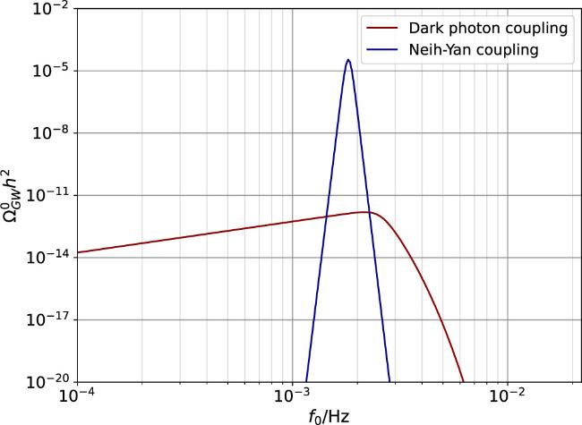
Figure 1. The broken power-law fitted curves of the SGWB for the dark photon (red) and Nieh–Yan (blue) coupling models, each using two parameter sets as described in sections |
3. Network of space-based GW detectors
In this section, we adopt the commonly used orbits of LISA and Taiji, combining them to evaluate their effectiveness in detecting the SGWB. We establish the coordinate system in the Solar System Barycentric Coordinate System (SSB). LISA trails the Earth by 20 degrees, and Taiji leads by the same degree, with both detector planes tilted 60 degrees relative to the ecliptic plane. The LISA-Taiji network configuration is displayed as figure 2.
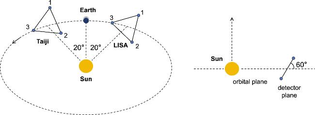
Figure 2. The configuration of the LISA-Taiji joint network, including the spacecraft numbering scheme. LISA orbits 20 degrees behind the Earth, while Taiji precedes the Earth by the same angle. Both detector planes are inclined at 60 degrees relative to the ecliptic plane. |
3.1. Noise and sensitivity of the detectors
Each detector contains three interferometers that simultaneously detect the Doppler shift induced by GWs. The data stream of Time-Delay Interferometry (TDI) channel i is given by A.2 . ${\tilde{{\rm{\Gamma }}}}_{ij}^{\lambda }(k)$ denotes the geometrical contribution to the detector response function for the correlation between channels i and j, as detailed in equation (A11 ).
$\begin{eqnarray}{d}_{i}(t)={s}_{i}(t)+{n}_{i}(t),\end{eqnarray}$
where si(t) represents the signal and ni(t) denotes the instrumental noise. In general, it is more convenient to work in the frequency domain $\begin{eqnarray}{\tilde{d}}_{i}(f)={\int }_{-T/2}^{T/2}{\rm{d}}t\,{{\rm{e}}}^{2\pi {\rm{i}}ft}{d}_{i}(t),\end{eqnarray}$
where T represents the observation time. In this paper, we assume that the noise is Gaussian and uncorrelated. The respective correlations of the signal and noise in the frequency domain can be expressed as $\begin{eqnarray}\begin{array}{rcl}\left\langle {\tilde{s}}_{i}(f){\tilde{s}}_{j}^{* }\left({f}^{{\prime} }\right)\right\rangle & = & \frac{1}{2}{S}_{ij}(f)\delta \left(f-{f}^{{\prime} }\right),\\ \left\langle {\tilde{n}}_{i}(f){\tilde{n}}_{j}^{* }\left({f}^{{\prime} }\right)\right\rangle & = & \frac{1}{2}{N}_{i}(f){\delta }_{ij}\delta \left(f-{f}^{{\prime} }\right),\end{array}\end{eqnarray}$
where Sij(f) and Ni(f) are the one-sided signal and noise power spectral density (PSD), respectively. Assuming independent TDI channel noises (e.g., in the A, E, T combination, which are the optimal TDI variables for LISA-like detectors), Sij(f) can be expressed as $\begin{eqnarray}\begin{array}{l}{S}_{ij}(f)=\displaystyle \sum _{\lambda }{P}_{\lambda }(f){{\rm{\Gamma }}}_{ij}^{\lambda }(f)=\displaystyle \sum _{\lambda }{P}_{\lambda }(f)\\ \times \,\left[\left(2\pi k{L}_{i}\right)\left(2\pi k{L}_{j}\right)W\left(k{L}_{i}\right){W}^{* }\left(k{L}_{j}\right){\tilde{{\rm{\Gamma }}}}_{ij}^{\lambda }(f)+\,\rm{h.c.}\,\right].\end{array}\end{eqnarray}$
Here, k = f/c, λ = L or R identifies left- and right-handed polarizations, Li and Lj are the detector arm lengths, ${{\rm{\Gamma }}}_{ij}^{\lambda }(f)$ is the full detector response function and Pλ(f) is the GW power spectrum. The function W(kL) represents the phase delay due to the detector arm length, as detailed in appendix In this work, we adopt the standard two-parameter noise model used for LISA, which accounts for the two dominant noise sources in space-based GW detectors: acceleration (acc) noise and Optical Measurement System (OMS) noise. For Taiji, we use a similar noise model with distinct parameters Aacc and AOMS. The acceleration noise power spectrum Pacc(f) and OMS noise power spectrum POMS(f) are given by [92, 93]
$\begin{eqnarray}\begin{array}{rcl}{P}_{{\rm{acc}}}(f) & = & {A}_{{\rm{acc}}}^{2}\left[1+{\left(\frac{0.4{\rm{mHz}}}{f}\right)}^{2}\right]{\left(\frac{2\pi f}{c}\right)}^{2}\\ & & \times \left[1+{\left(\frac{f}{8{\rm{mHz}}}\right)}^{4}\right]{\left(\frac{1}{2\pi f}\right)}^{4},\end{array}\end{eqnarray}$
$\begin{eqnarray}{P}_{{\rm{OMS}}}(f)={A}_{{\rm{OMS}}}^{2}\left[1+{\left(\frac{2{\rm{mHz}}}{f}\right)}^{4}\right]{\left(\frac{2\pi f}{c}\right)}^{2}.\end{eqnarray}$
Here, Aacc and AOMS are the amplitudes of the acceleration noise and the OMS noise, respectively. For the two detectors, the noise amplitude parameters for LISA [94] and Taiji [70, 95, 96] are listed in table 1.Table 1. Noise amplitude spectral density parameters and arm lengths for different space-based GW detectors. |
| AOMS | Aacc | L | |
|---|---|---|---|
| LISA | $15\,{\rm{pm}}/\sqrt{{\rm{Hz}}}$ | $3\,{\rm{fm}}/{{\rm{s}}}^{2}/\sqrt{{\rm{Hz}}}$ | 2.5 Gm |
| | |||
| Taiji | $8\,{\rm{pm}}/\sqrt{{\rm{Hz}}}$ | $3\,{\rm{fm}}/{{\rm{s}}}^{2}/\sqrt{{\rm{Hz}}}$ | 3.0 Gm |
For convenience, we define the detector’s characteristic frequency as f* ≡ c/2πL. The power spectral density of the noise for a single detector channel is then given by [13, 97]
$\begin{eqnarray}\begin{array}{l}\quad {N}_{{\rm{A}}}(f)={N}_{{\rm{E}}}(f)\\ =\,8{\sin }^{2}\left(\frac{f}{{f}_{* }}\right)\left\{4\left[1+\cos \left(\frac{f}{{f}_{* }}\right)+{\cos }^{2}\left(\frac{f}{{f}_{* }}\right)\right]\right.\\ \quad \quad \times \,{P}_{{\rm{acc}}}(f)\left.+\left[2+\cos \left(\frac{f}{{f}_{* }}\right)\right]\times {P}_{{\rm{OMS}}}(f)\right\},\end{array}\end{eqnarray}$
and $\begin{eqnarray}\begin{array}{rcl}{N}_{{\rm{T}}}(f) & = & 16{\sin }^{2}\left(\frac{f}{{f}_{* }}\right)\left\{2{\left[1-\cos \left(\frac{f}{{f}_{* }}\right)\right]}^{2}\right.\\ & & \left.\times {P}_{{\rm{acc}}}(f)+\left[1-\cos \left(\frac{f}{{f}_{* }}\right)\right]\times {P}_{{\rm{OMS}}}(f)\right\},\end{array}\end{eqnarray}$
where the subscripts A, E, and T denote the noise-orthogonal TDI channels A, E, and T, respectively. The space-based detector with three equal arms combines into three independent channels: A, E, and T. The A and E channels function as orthogonal interferometers sensitive to GW polarizations. Although their responses differ for GWs from specific directions, the all-sky averaged sensitivities of A and E channels are identical due to the detector’s rotational symmetry. As shown in figure 3(a), the T channel (Sagnac combination) remains insensitive to GWs at low frequencies while maintaining sensitivity to instrumental noise. This characteristic allows the T channel to help characterize and subtract instrumental noise, enhancing the overall detection capability, particularly for stochastic background measurements.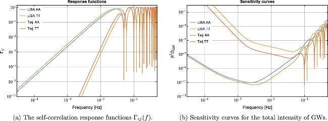
Figure 3. (a) The self-correlation response functions Γij in ( |
To directly compare incident GW signals with detector noise, we define the strain sensitivity of total intensity for all GW modes as [13]A14 ). The corresponding total intensity, in GW energy density units, is given by:
$\begin{eqnarray}{P}_{N,ii}(f)=\frac{{N}_{i}(f)}{{{\rm{\Gamma }}}_{ii}(f)}\,,\end{eqnarray}$
where Γii(f) represents the sky-averaged response functions of individual TDI channels, which can be calculated via equation ( $\begin{eqnarray}{h}^{2}{{\rm{\Omega }}}_{N,ii}(f)=\frac{4{\pi }^{2}{f}^{3}}{3{\left({H}_{0}/h\right)}^{2}}{P}_{N,ii}(f)\,,\end{eqnarray}$
where H0 = h 100 km s−1 Mpc−1 is the value of the present-day Hubble parameter and h = 0.67 is the dimensionless Hubble parameter. Figure 3 shows the total intensity sensitivity curves for the A and E channels of both LISA and Taiji. Similarly, the SGWB adopts a similar notation, with PN,ij replaced by the GW power spectrum [61] $\begin{eqnarray}{h}^{2}{{\rm{\Omega }}}_{{\rm{GW}}}^{\lambda }(f)=\frac{4{\pi }^{2}{f}^{3}}{3{({H}_{0}/h)}^{2}}{P}_{\lambda }(f)\,.\end{eqnarray}$
3.2. LISA-taiji cross-correlations
Individual detectors like LISA or Taiji are insensitive to GW chiral signatures due to their planar configuration. The three arms of LISA form a plane, and this geometry inherently lacks sensitivity to isotropic chiral GWB. For example, left-handed circularly polarized signals of equal intensity from opposite directions incident on the detector plane would cancel their chiral signatures. Taiji, with a similar configuration, shares this limitation. However, when two spatially separated detectors form a non-coplanar network, the combined system gains sensitivity to the Stokes V parameter, characterizing GW chirality. This non-coplanar configuration of the LISA-Taiji network enables detection of isotropic chiral GWB that remains undetectable by individual detectors.
We use the Stokes parameters I(f) and V(f) to characterize the polarization of the SGWB in the cross-correlated detector data stream. They are defined as 12 ) for ${\tilde{{\rm{\Gamma }}}}_{ij}^{\lambda }(f)$ can be reformulated using the Stokes parameters I and V, with λ = I, V. By cross-correlating the signals from LISA and Taiji channels, we can extract nonzero ${\tilde{{\rm{\Gamma }}}}_{ij}^{V}(f)$ values. The I and V components resulting from this cross-correlation of all TDI channels between LISA and Taiji are presented in figure 4.
$\begin{eqnarray}I(f)={P}_{R}(f)+{P}_{L}(f),\quad V(f)={P}_{R}(f)-{P}_{L}(f).\end{eqnarray}$
Here, I represents the total intensity of the GW, while V quantifies the difference between right-handed and left-handed circular polarization intensities. Parity-violating effects in the early Universe may give rise to a nonzero value of V. By using detectors to measure it, we can extract information about the circular polarization of GWs. We can express GW power spectral density Sij as $\begin{eqnarray}{S}_{ij}(f)=I(f){{\rm{\Gamma }}}_{ij}^{I}(f)+V(f){{\rm{\Gamma }}}_{ij}^{V}(f),\end{eqnarray}$
where ${{\rm{\Gamma }}}_{ij}^{I}(f)$ and ${{\rm{\Gamma }}}_{ij}^{V}(f)$ are the overlap reduction functions for intensity and circular polarization components, quantifying the correlated response between TDI channels i and j. These functions are defined as: $\begin{eqnarray}\begin{array}{rcl}{{\rm{\Gamma }}}_{ij}^{I}(f) & = & \frac{{{\rm{\Gamma }}}_{ij}^{R}(f)+{{\rm{\Gamma }}}_{ij}^{L}(f)}{2},\\ {{\rm{\Gamma }}}_{ij}^{V}(f) & = & \frac{{{\rm{\Gamma }}}_{ij}^{R}(f)-{{\rm{\Gamma }}}_{ij}^{L}(f)}{2}.\end{array}\end{eqnarray}$
Thus, the power spectral density in equation (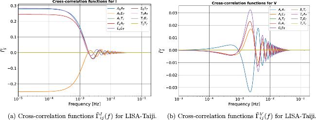
Figure 4. Cross-correlation functions ${\tilde{{\rm{\Gamma }}}}_{ij}^{\lambda }(f)$ in equation ( |
Additionally, we introduce the circular polarization parameter as
$\begin{eqnarray}{\rm{\Pi }}(f)=\frac{V(f)}{I(f)}.\end{eqnarray}$
The correlation between the outputs of different detectors can be expressed as: $\begin{eqnarray}\left\langle {{ \mathcal C }}_{ij}\right\rangle =\left\langle {\tilde{d}}_{i}{\tilde{d}}_{j}\right\rangle =\frac{1}{2}\left[{{\rm{\Gamma }}}_{ij}^{I}(f)I(f)+{{\rm{\Gamma }}}_{ij}^{V}(f)V(f)\right].\end{eqnarray}$
Assuming that the noise is Gaussian, the likelihood function of the signal model is [98]25 ) is replaced by [98–100]
$\begin{eqnarray}\begin{array}{rcl}{ \mathcal L } & = & p({ \mathcal C }| \theta )\\ & \propto & \exp \left\{-\frac{{T}_{{\rm{obs}}}}{2}\displaystyle \sum _{\kappa }{\displaystyle \int }_{0}^{\infty }{\rm{d}}f\frac{{\left[2{{ \mathcal C }}_{\kappa }-\left({{\rm{\Gamma }}}_{\kappa }^{I}I+{{\rm{\Gamma }}}_{\kappa }^{V}V\right)\right]}^{2}}{{N}_{\kappa }^{2}(f)}\right\},\end{array}\end{eqnarray}$
where κ = {AL − AT, AL − ET, EL − AT, EL − ET} represents the independent channel pairs of LISA and Taiji. With AL and EL denoting the LISA channels and AT and ET corresponding to the Taiji channels. Tobs denotes the effective observation time, which is set to 3 years in this work. The noise term Nκ(f) is defined as ${N}_{\kappa }(f)=\sqrt{{N}_{i}\left(f\right){N}_{j}\left(f\right)}$. For strong GW signal, such as an SGWB with a large signal-to-noise ratio (SNR), ${N}_{\kappa }^{2}(f)$ in ( $\begin{eqnarray}{M}_{ij}(f)=({N}_{i}+{{\rm{\Gamma }}}_{ii}I)({N}_{j}+{{\rm{\Gamma }}}_{jj}I)+{\left({{\rm{\Gamma }}}_{ij}^{I}I+{{\rm{\Gamma }}}_{ij}^{V}V\right)}^{2}.\end{eqnarray}$
4. Fisher matrix analysis
In this section, we employ Fisher matrix analysis to estimate the measurement accuracy of the GW spectral parameters. The Fisher matrix is given by as [61, 98]
$\begin{eqnarray}{F}_{ab}=-\displaystyle \sum _{\kappa }4{T}_{\,\rm{obs}\,}{\int }_{0}^{\infty }{\rm{d}}f\frac{\frac{\partial \left\langle {C}_{\kappa }\right\rangle }{\partial {\theta }_{a}}\frac{\partial \left\langle {C}_{\kappa }\right\rangle }{\partial {\theta }_{b}}}{{N}_{\kappa }^{2}(f)},\end{eqnarray}$
where θa and θb are the model parameters. The term Cκ is the correlation of the observed data between the κ channel sets, and Nκ(f) represents the signal variance caused by noise. For the frequency integration, we take the lower cutoff at 10−5 Hz and the upper cutoff at 10−1 Hz. In this study, we assume a frequency-independent circular polarization parameter Π(f) = Π and derive the Fisher matrix expression for the GW model parameters as follows.By substituting the signal equation (19 ), the circular polarization parameter in equation (23 ), and equation (24 ), we have
$\begin{eqnarray}\begin{array}{rcl}{F}_{ab} & = & 4{T}_{{\rm{obs}}}{\left(\frac{3{H}_{0}^{2}}{4{\pi }^{2}}\right)}^{2}\\ & & \times \displaystyle \sum _{\kappa }{\displaystyle \int }_{0}^{\infty }{\rm{d}}f\frac{{\left({{\rm{\Gamma }}}_{\kappa }^{I}+{\rm{\Pi }}\,{{\rm{\Gamma }}}_{\kappa }^{V}\right)}^{2}{\partial }_{{\theta }_{a}}{\rm{\Omega }}\left(f\right){\partial }_{{\theta }_{b}}{\rm{\Omega }}\left(f\right)}{{f}^{6}\,{N}_{\kappa }^{2}},\end{array}\end{eqnarray}$
with a and b indicate both parameters of the GW model. For example, when one parameter is Π and the other is a GW model parameter $\begin{eqnarray}\begin{array}{rcl}{F}_{a{\rm{\Pi }}} & = & 4{T}_{{\rm{obs}}}{\left(\frac{3{H}_{0}^{2}}{4{\pi }^{2}}\right)}^{2}\\ & & \times \displaystyle \sum _{\kappa }{\displaystyle \int }_{0}^{\infty }{\rm{d}}f\frac{{{\rm{\Gamma }}}_{\kappa }^{V}\left({{\rm{\Gamma }}}_{\kappa }^{I}+{\rm{\Pi }}\,{{\rm{\Gamma }}}_{\kappa }^{V}\right)\,{\rm{\Omega }}\left(f\right){\partial }_{{\theta }_{a}}{\rm{\Omega }}\left(f\right)}{{f}^{6}\,{N}_{\kappa }^{2}}.\end{array}\end{eqnarray}$
When both parameters in the Fisher matrix are Π $\begin{eqnarray}{F}_{{\rm{\Pi }}{\rm{\Pi }}}=4{T}_{{\rm{obs}}}{\left(\frac{3{H}_{0}^{2}}{4{\pi }^{2}}\right)}^{2}\displaystyle \sum _{\kappa }{\int }_{0}^{\infty }{\rm{d}}f\frac{{\left({{\rm{\Gamma }}}_{\kappa }^{V}\right)}^{2}{\rm{\Omega }}{\left(f\right)}^{2}}{{f}^{6}\,{N}_{\kappa }^{2}}.\end{eqnarray}$
4.1. GW spectral parameters
We selected the spectral parameters of the GW template for parameter estimation, as detailed in table 2, and the results from the Fisher analysis of the GW energy density spectrum template (2 ) for audible axion are illustrated in figure 5. Our nearly maximally polarized signal (Π = 0.9999) arises from the tachyonic instability due to the axion-like terms in [32, 52], where axion oscillations cause one helicity mode to grow exponentially, generating a highly chiral GW background. Simulations of both dark photon and Nieh–Yan couplings validate this high polarization degree.
Table 2. Parameter values for the broken power-law template ( |
| As | fs | γ | p | Π |
| | ||||
| 6.3 | 2.0 | 12.9 | 1.5 | 0.9999 |
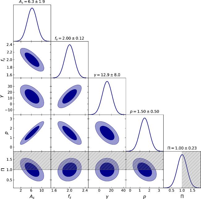
Figure 5. Corner plots of SGWB spectral parameters estimates for the dark photon coupling model derived from the Fisher matrix, with parameter values listed in table 2. At the top of each column, the corresponding parameters’ 1σ uncertainty are presented. The gray shaded areas correspond to regions of the parameter space with Π > 1, which is theoretically unacceptable. |
For the dark photon coupling model, the uncertainties in the parameter estimates are illustrated graphically, encompassing four spectral parameters $\left\{{A}_{s},{f}_{s},\gamma ,p\right\}$ and the circular polarization parameter Π. The confidence ellipses indicate that the true parameter values lie within the inner ellipse at a 1σ confidence level and within the outer ellipse at a 2σ confidence level. At the 1σ confidence level, the relative errors are less than 62.0% for spectral parameters and less than 23.0% for Π. The elongation of the confidence ellipses reflects the strength of the correlation among spectral parameters, with more elongated ellipses indicating stronger correlations. Specifically, p and As exhibit a strong correlation. Additionally, the Π is negatively correlated with As, p, shows a weak negative correlation with γ and is independent of fs. In figures 5, 6, 7(a), and (b), the gray solid line represents the fiducial value Π = 1, representing a fully polarized state. The gray shaded areas in the corner plots correspond to regions of the parameter space where Π > 1, which is theoretically unacceptable.
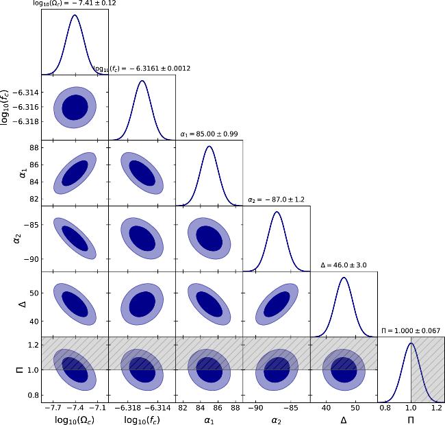
Figure 6. Corner plots of SGWB spectral parameters estimates for the Nieh–Yan coupling model derived from the Fisher matrix, with parameter values listed in table 3. At the top of each column, the corresponding parameters’ 1σ uncertainty is presented. The gray shaded areas correspond to regions of the parameter space with Π > 1, which is theoretically unacceptable. |
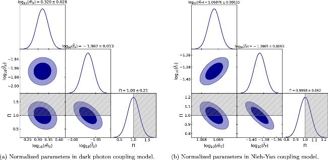
Figure 7. Corner plots showing SGWB normalized model parameters estimates from the Fisher matrix for (a) the dark photon coupling model and (b) the Nieh–Yan coupling model in table 4. At the top of each column, the corresponding parameters’ 1σ uncertainties are presented. The gray shaded areas correspond to regions of the parameter space with Π > 1 which is theoretically unacceptable. |
For the broken power-law template in the Nieh–Yan coupling models, we also have selected the spectral parameters as shown in table 3, with the corresponding Fisher analysis results presented in figure 6. The direct coupling of the axion to the gravitational field in equation (5 ) and the parameter choices in table 3 result in a strong signal, making the variance assumption invalid. Therefore, the noise term ${N}_{\kappa }^{2}$ in our Fisher matrix is replaced by Mκ(f) in equation (26 ). The Fisher analysis results for the GW energy density spectrum in the Nieh–Yan coupling model are shown in figure 6. At the 1σ confidence level, the relative errors are less than 31.8% for spectral parameters and less than 6.7% for Π. Ωc and fc exhibit relatively independent errors, while other spectral parameters show significant correlations. Furthermore, the circular polarization parameter Π exhibits a negative correlation with Ωc and fc, a statistically weak correlation with α1 and α2, and no correlation with Δ.
Table 3. Parameter values for the broken power-law template ( |
| Ωc | fc/mHz | α1 | α2 | Δ | Π |
|---|---|---|---|---|---|
| 6.072 × 10⁻⁴ | 1.807 | 85 | −87 | 46 | 0.9999 |
4.2. Normalized model parameters
Based on the relationship between the spectral parameters and the physical parameters, the equations (3 ) and (4 ) for the dark photon couplings, as well as equations (7 ) and (8 ) for the Nieh–Yan coupling, which enables us to constrain the physical parameters via measurements of the spectral shape.
We introduce the dimensionless normalized model parameters by combining the axion mass m, the coupling constant αX/T, and the decay constant fX/T as follows2 ) and (6 ). From the specific physical parameters of the dark photon coupling and the Nieh–Yan coupling models, as described in sections 2.1 and 2.2 respectively, we obtain the values of these dimensionless normalized model parameters, which are explicitly listed in table 4. We use the Fisher matrix to estimate the normalized model parameters.
$\begin{eqnarray}{\tilde{m}}_{X/T}=\frac{m}{\,\rm{eV}\,}{\left(\frac{{\alpha }_{X/T}}{{M}_{P}^{2}}\right)}^{4/3},\end{eqnarray}$
$\begin{eqnarray}{\tilde{f}}_{X}=\frac{{f}_{X}}{{M}_{P}}{\left(\frac{{\alpha }_{X}}{{M}_{P}^{2}}\right)}^{-\frac{1}{3}},\,\,{\tilde{f}}_{T}=\frac{{f}_{T}}{{M}_{P}},\end{eqnarray}$
and substitute them into the spectral form (Table 4. Values of the normalized model parameters for dark photon coupling and Nieh–Yan coupling models. The subscript ${ \mathcal O }$ in ${\tilde{m}}_{{ \mathcal O }}$ and ${\tilde{f}}_{{ \mathcal O }}$ denotes the model index: ${ \mathcal O }=X$ for dark photon coupling, ${ \mathcal O }=T$ for Nieh–Yan coupling. |
| ${\tilde{m}}_{{ \mathcal O }}$ | ${\tilde{f}}_{{ \mathcal O }}$ | Π | |
|---|---|---|---|
| X(Dark Photon) | 2.092 | 0.0108 | 0.9999 |
| | |||
| T(Nieh–Yan) | 11.72 | 0.0411 | 0.9999 |
We compute the Fisher matrix of the normalized model parameters $\tilde{m}$, ${\tilde{f}}_{X}$, and ${\tilde{f}}_{T}$ to obtain its covariance matrix. The correlation plots of this matrix are shown in figures 7(a) and (b). We can constrain the values of the physical parameters by the measurement of these normalized model parameters.
For dark photon coupling model as given in equation (2 ), the results are shown in figure 7(a). At the 1σ confidence level, the relative errors are less than 6.7% for the normalized model parameters. It can be observed that the measurements of ${\tilde{m}}_{X}$ and ${\tilde{f}}_{X}$ are approximately independent, whereas Π exhibits a certain degree of negative correlation with both ${\tilde{m}}_{X}$ and ${\tilde{f}}_{X}$. The parameter Π is estimated to be 0.9999 with a relative uncertainty of 21.0% at the 1σ confidence level. To improve the measurement precision of Π, we can enhance the sensitivity of individual detectors and the detector network, as well as achieve higher SNR.
For the Nieh–Yan coupling model, the result for the broken power-law template in equation (6 ) is shown in figure 7. At the 1σ confidence level, the relative errors are less than 2.2% for the normalized model parameters. It can be observed that the measurements of the parameters ${\tilde{m}}_{T}$, ${\tilde{f}}_{T}$, and Π are correlated. Moreover, due to the strong signal strength, the measurement precision of Π has been improved compared to the results for the dark photon coupling model, with a relative error of 6.2% at the 1σ confidence level. Meanwhile, we can see that the measurement precision of ${\tilde{m}}_{T}$ is relatively high. This is because the broken power-law template has a narrow peak and strong amplitude at the peak frequency, measuring the peak frequency more sensitive. According to the relationships (7 ) and (31 ), it is clear that $\tilde{m}$ corresponds to the measurement of the peak frequency.
5. Conclusion
The single GW detectors face challenges in detecting the chirality of GWs due to their planar design. However, with the network of space-based detectors such as LISA and Taiji through cross-correlation techniques, we can compute chirality-dependent response functions and extract the net circular polarization of an isotropic SGWB. The detection of parity violation through chiral GWs is crucial for understanding the early Universe and for distinguishing a cosmological GW background from an astrophysical one. In this work, we present the response functions for Stokes parameters I and V, as well as the total intensity sensitivity curve for GWBs originating from audible axions, using the LISA-Taiji network. In addition to the LISA-Taiji network, other space-based GW detector networks such as LISA-TianQin have also been proposed and studied extensively [101–104].
We use the Fisher information matrix to estimate both spectral parameters and normalized model parameters of axion-induced chiral GW spectra through the LISA-Taiji network, focusing on axion-dark photon and axion-Nieh–Yan couplings with physical parameters selected to yield strong GWs in the mHz range. Our results demonstrate that the network estimates the spectral shape parameters and normalized model parameters for both coupling models. For the spectral shape parameters in the dark photon coupling model, we obtain relative errors of 62.0% at the 1σ confidence level, while for the Nieh–Yan coupling model, the relative errors are less than 31.8% at the same confidence level. Regarding circular polarization parameter Π, its relative error is less than 23.0% (1σ) for the dark photon coupling model, and it is reduced to 6.7% (1σ) for the stronger signals from the Nieh–Yan coupling model. Compared to flat GW spectra in [61], we have computed the parameter uncertainties for frequency-dependent spectra of the axion-induced chiral GWB, demonstrating the LISA-Taiji network’s capability to effectively constrain both GW spectral parameters and normalized model parameters.
Appendix. Response functions of GWs
In this work, we employ natural units and adopt the Lorentz transverse-traceless gauge. We establish a coordinate system $\left\{{\hat{e}}_{x},{\hat{e}}_{y},{\hat{e}}_{z}\right\}$ at rest relative to an isotropic SGWB.
A.1. Polarization tensor bases
For an incoming plane GW with a single wave vector $\overrightarrow{k}$, we define an orthogonal basis
$\begin{eqnarray}\hat{u}(\hat{k})=\frac{\hat{k}\times {\hat{e}}_{z}}{| \hat{k}\times {\hat{e}}_{z}| },\quad \hat{v}(\hat{k})=\hat{k}\times \hat{u},\end{eqnarray}$
where $\hat{k}$ denotes the unit vector in the direction of wave-vector $\overrightarrow{k}$, and its magnitude is given by $k=| \overrightarrow{k}| $. Using the above equation, we define the so-called ‘plus’ (+) and ‘cross’ (×) polarization tensors as $\begin{eqnarray}{e}_{ab}^{+}(\hat{k})=\frac{{\hat{u}}_{a}{\hat{u}}_{b}-{\hat{v}}_{a}{\hat{v}}_{b}}{\sqrt{2}},\quad {e}_{ab}^{\times }(\hat{k})=\frac{{\hat{u}}_{a}{\hat{v}}_{b}+{\hat{v}}_{a}{\hat{u}}_{b}}{\sqrt{2}}.\end{eqnarray}$
It is more convenient to introduce the circular polarization basis tensors ${e}_{ab}^{R}$ and ${e}_{ab}^{L}$ when searching for evidence of circular polarization in the background. Then the relationships between the left- and right-handed polarization tensors and the ‘plus’ (+) and ‘cross’ (×) polarization basis are
$\begin{eqnarray}{e}_{ab}^{R}(\hat{k})=\frac{{e}_{ab}^{+}+{\rm{i}}{e}_{ab}^{\times }}{\sqrt{2}},\quad {e}_{ab}^{L}(\hat{k})=\frac{{e}_{ab}^{+}-{\rm{i}}{e}_{ab}^{\times }}{\sqrt{2}}.\end{eqnarray}$
The superposition of GWs arriving at position $\overrightarrow{x}$ at time t can be represented as an incident plane wave
$\begin{eqnarray}{h}_{ab}(\overrightarrow{x},t)={\int }_{-\infty }^{+\infty }{\rm{d}}f{\int }_{{\rm{\Omega }}}{\rm{d}}{{\rm{\Omega }}}_{\hat{k}}\,{{\rm{e}}}^{2\pi {\rm{i}}f(t-\hat{k}\cdot \overrightarrow{x})}\displaystyle \sum _{P}{\tilde{h}}_{P}(f,\hat{k}){e}_{ab}^{P}(\hat{k}),\end{eqnarray}$
where the index P labels either the plus and cross polarizations (+/×) or the left- and right-handed polarizations (L/R). Here, f = k c denotes the frequency of each plane wave, ${\rm{d}}{{\rm{\Omega }}}_{\hat{k}}$ represents the infinitesimal solid angle corresponding to the wave vector $\overrightarrow{k}$, and ${\tilde{h}}_{P}(f,\hat{k})\equiv {f}^{2}{\tilde{h}}_{P}(\overrightarrow{k})$. Finally, the gravitational wave can be expressed in terms of $\overrightarrow{k}$ as $\begin{eqnarray}\begin{array}{rcl}{h}_{ab}(\overrightarrow{x},t) & = & \displaystyle \int {{\rm{d}}}^{3}k\,{{\rm{e}}}^{-2\pi {\rm{i}}\overrightarrow{k}\cdot \overrightarrow{x}}\displaystyle \sum _{P}\left[{{\rm{e}}}^{2\pi {\rm{i}}kt}{\tilde{h}}_{P}(\overrightarrow{k}){e}_{ab}^{P}(\hat{k})\right.\\ & & \left.+{{\rm{e}}}^{-2\pi {\rm{i}}kt}{\tilde{h}}_{P}^{* }(-\overrightarrow{k}){e}_{ab}^{P* }(-\hat{k})\right].\end{array}\end{eqnarray}$
A.2. Quadratic response functions
In actual measurements, space-based detectors measure differential Doppler frequency shifts rather than direct time shifts. These shifts are defined as ΔF12(t) ≡ Δν12(t)/ν = − dΔT12(t)/dt. We use L to denote the detector arm length. The most straightforward interferometric measurement at a vertex performed by a space-based detector is
$\begin{eqnarray}\begin{array}{rcl}{\rm{\Delta }}{F}_{1(23)}(t) & = & {\rm{\Delta }}{F}_{21}(t-L)+{\rm{\Delta }}{F}_{12}(t)\\ & & -\left[{\rm{\Delta }}{F}_{31}(t-L)+{\rm{\Delta }}{F}_{13}(t)\right].\end{array}\end{eqnarray}$
In order to suppress noise induced by laser phase variations and other factors, we implement TDI techniques. Consider two test masses labeled i and j, and let ${\hat{l}}_{ij}=\left({{\boldsymbol{x}}}_{j}-{{\boldsymbol{x}}}_{i}\right)/\left|{{\boldsymbol{x}}}_{j}-{{\boldsymbol{x}}}_{i}\right|$ denote the unit vector pointing from mass i to mass j among the three detector spacecraft. The TDI1.5 variable is obtained through cyclic permutation of the TDI variables Y and Z
$\begin{eqnarray}\begin{array}{l}\quad {\rm{\Delta }}{F}_{1(23)}^{1.5}(t)={\rm{\Delta }}{F}_{1(23)}(t-2L)+{\rm{\Delta }}{F}_{1(32)}(t)\\ =-\displaystyle \int {{\rm{d}}}^{3}k\,{{\rm{e}}}^{-2\pi {\rm{i}}\overrightarrow{k}\cdot {\overrightarrow{x}}_{1}}(2\pi {\rm{i}}kL)\\ \,\times \,\displaystyle \sum _{\lambda }\left[{{\rm{e}}}^{2\pi {\rm{i}}k(t-L)}W(kL){R}_{1}^{\lambda }(\overrightarrow{k},{\hat{l}}_{12},{\hat{l}}_{13}){\tilde{h}}_{\lambda }(k)\right.\\ \quad \left.-{{\rm{e}}}^{-2\pi {\rm{i}}k(t-L)}{W}^{* }(kL){R}_{1}^{{\lambda }^{* }}(-\overrightarrow{k},{\hat{l}}_{12},{\hat{l}}_{13}){\tilde{h}}_{\lambda }^{* }(-k)\right].\end{array}\end{eqnarray}$
where λ = L or R denotes left- and right-handed polarizations, and W(kL) ≡ e−4πikL − 1. The function ${R}_{i}^{\lambda }$ is defined as $\begin{eqnarray}{R}_{i}^{\lambda }(\overrightarrow{k},{\hat{l}}_{ij},{\hat{l}}_{ik})\equiv \frac{{\hat{l}}_{ij}^{a}{\hat{l}}_{ij}^{b}}{2}{e}_{ab}^{\lambda }(\hat{k}){ \mathcal T }(\overrightarrow{k},{\hat{l}}_{ij})-\frac{{\hat{l}}_{ik}^{a}{\hat{l}}_{ik}^{b}}{2}{e}_{ab}^{\lambda }(\hat{k}){ \mathcal T }(\overrightarrow{k},{\hat{l}}_{ik}),\end{eqnarray}$
where the detector transfer function ${ \mathcal T }(\overrightarrow{k},{\hat{l}}_{ij})$ is given by $\begin{eqnarray}\begin{array}{rcl}{ \mathcal T }(\overrightarrow{k},{\hat{l}}_{ij}) & \equiv & {{\rm{e}}}^{\pi {\rm{i}}kL\left(1-\hat{k}\cdot {\hat{l}}_{ij}\right)}\mathrm{sinc}\left[\pi kL\left(1+\hat{k}\cdot {\hat{l}}_{ij}\right)\right]\\ & & +\,{{\rm{e}}}^{-\pi {\rm{i}}kL\left(1+\hat{k}\cdot {\hat{l}}_{ij}\right)}\mathrm{sinc}\left[\pi kL\left(1-\hat{k}\cdot {\hat{l}}_{ij}\right)\right].\end{array}\end{eqnarray}$
For simplicity, we represent the detector output using the notation ${s}_{i}(t)\equiv {\rm{\Delta }}{F}_{i(jk)}^{1.5}(t)$. The information is contained within the two-point correlation functions of the data streams. Below, without assuming identical detectors, we present the general formulation. The two-point cross-correlation is expressed as
$\begin{eqnarray}\begin{array}{l}\left\langle {s}_{i}(t){s}_{j}(t)\right\rangle =\displaystyle \int {\rm{d}}k\,(2\pi k{L}_{i})(2\pi k{L}_{j})\displaystyle \sum _{\lambda }{P}_{\lambda }(k)\\ \quad \times \,\left[{{\rm{e}}}^{-2\pi {\rm{i}}k({L}_{i}-{L}_{j})}W(k{L}_{i}){W}^{* }(k{L}_{j}){\tilde{{\rm{\Gamma }}}}_{ij}^{\lambda }(k)+\,\rm{h.c.}\,\right],\end{array}\end{eqnarray}$
where the cross-correlation function $\begin{eqnarray}\begin{array}{rcl}{\tilde{{\rm{\Gamma }}}}_{ij}^{\lambda }(k) & \equiv & \frac{1}{4\pi }\displaystyle \int {{\rm{d}}}^{2}\hat{k}\,{{\rm{e}}}^{-2\pi {\rm{i}}\overrightarrow{k}\cdot \left({\overrightarrow{x}}_{i}-{\overrightarrow{x}}_{j}\right)}\\ & & \times \,{R}_{i}^{\lambda }\left(\overrightarrow{k},{\hat{l}}_{ik},{\hat{l}}_{il}\right){R}_{j}^{{\lambda }^{* }}\left(\overrightarrow{k},{\hat{l}}_{jm},{\hat{l}}_{jn}\right).\end{array}\end{eqnarray}$
For notational simplicity, the quadratic response function $\begin{eqnarray}{{\rm{\Gamma }}}_{ij}^{\lambda }(k)\equiv \,(2\pi k{L}_{i})(2\pi k{L}_{j})W(k{L}_{i}){W}^{* }(k{L}_{j}){\tilde{{\rm{\Gamma }}}}_{ij}^{\lambda }(k)+\,\rm{h.c.},\end{eqnarray}$
we obtain the compact form $\begin{eqnarray}\langle {s}_{i}(t){s}_{j}(t)\rangle =\int {\rm{d}}k\left[{{\rm{\Gamma }}}_{ij}^{L}(k){P}_{L}(k)+{{\rm{\Gamma }}}_{ij}^{R}(k){P}_{R}(k)\right].\end{eqnarray}$
When i and j are both LISA (or Taiji) channels, the response function is given by $\begin{eqnarray}\begin{array}{rcl}{{\rm{\Gamma }}}_{ij}(k) & = & {{\rm{\Gamma }}}_{ij}^{L}(k)+{{\rm{\Gamma }}}_{ij}^{R}(k)\\ & = & 16{(2\pi kL)}^{2}{\sin }^{2}(2\pi kL){\tilde{{\rm{\Gamma }}}}_{ij}(k),\end{array}\end{eqnarray}$
where ${\tilde{{\rm{\Gamma }}}}_{ij}(k)={\tilde{{\rm{\Gamma }}}}_{ij}^{L}(k)={\tilde{{\rm{\Gamma }}}}_{ij}^{R}(k)$ [13]. The response functions Γij for the A and E channels of LISA and Taiji are shown in figure 3(a).Using the methods in [61, 105], we have calculated the response functions and total intensity sensitivity curves associated with the self-correlation of LISA and Taiji. The corresponding results are shown in figure 3. Additionally, we have obtained the response functions for the I and V components of all cross-correlation TDI channels between LISA and Taiji, as shown in figure 4. For further details on the derivation, we refer to [13, 61].
A.3. The AET bases
In space-based gravitational wave detection, the fundamental TDI channels of a Michelson interferometer include X, Y, and Z. We transform the X, Y, and Z channels into the noise-independent channels A, E, and T, which are related as follows [61]
$\begin{eqnarray}{\tilde{d}}_{A}=\frac{1}{\sqrt{2}}({\tilde{d}}_{Z}-{\tilde{d}}_{X}),\end{eqnarray}$
$\begin{eqnarray}{\tilde{d}}_{E}=\frac{1}{\sqrt{6}}({\tilde{d}}_{X}-2{\tilde{d}}_{Y}+{\tilde{d}}_{Z}),\end{eqnarray}$
$\begin{eqnarray}{\tilde{d}}_{T}=\frac{1}{\sqrt{3}}({\tilde{d}}_{X}+{\tilde{d}}_{Y}+{\tilde{d}}_{Z}).\end{eqnarray}$
The noise independence of the A, E, and T channels is valid under the assumptions of identical noise in each laser link and equal arm lengths.For convenience, we summarize the key symbols used in this paper in table 5.
Table 5. Summary of the symbols and descriptions. |
| Symbols | Descriptions |
|---|---|
| Sij(f) | One-sided signal power spectral density |
| | |
| Ni(f) | One-sided noise power spectral density |
| | |
| ${h}_{ab}(\overrightarrow{x},t)$ | Gravitational wave strain tensor |
| | |
| ΔFij(t) | Doppler frequency shifts |
| | |
| ${\tilde{{\rm{\Gamma }}}}_{ij}^{\lambda }(k)$ | Cross-correlation function |
| | |
| ${{\rm{\Gamma }}}_{ij}^{\lambda }(k)$ | Quadratic response function |