


This work is devoted to exploring the possible pathway to ergodicity in nonlinear systems through chaotic dynamics, and question whether chaotic dynamics are sufficient for this goal [1, 2]; see figure 1. We also explore the possible signature that can be achieved in experiments. In statistical physics, ergodicity ensures that for any operator A, its average $\bar{A}$ can be calculated using both time average and ensemble average [2–7]
$\begin{eqnarray}\bar{A}=\mathop{\mathrm{lim}}\limits_{T\to \infty }\frac{1}{T}{\int }_{0}^{T}A(t){\rm{d}}t={\int }_{{\rm{\Gamma }}}\rho (x)A(x){\rm{d}}x,\end{eqnarray}$
where ρ(x) represents the probability density in the phase space Γ and A(x) is the observable at point x. In this formula, the distribution ρ(x) is essential for the above identity. In ergodic systems, the time average over a trajectory equals the ensemble average across the entire phase space. Ergodicity provides a framework to understand the long-term average in different models [8]. However, in periodic or quasiperiodic systems, and in physical models with local conservation laws or local constraints [9], the (closed) orbit only visits a small portion of the phase space, leading to a failure of the above relation for breaking of ergodicity. In contrast, in the chaotic systems or in some models without integrability due to the many-body interactions, it is quite possible that the system may approach the ergodic condition when the dynamics are complicated enough. Therefore, the chaotic dynamics seem to provide a unique pathway to ergodicity in these models. In the previous literature, ergodicity in the many-body models have been explored using numerical methods and experiments [2, 10–13]; however, the conclusions suffer seriously from the finite size effect. For these reasons, it may have been widely believed that the ergodicity can only happen in large systems limit N → ∞ (or when N is large enough); see the original proof of ergodic theorem in [14–16]. This conclusion has also been noticed in the discussion section of the celebrated paper by Hoover for molecular dynamics [17].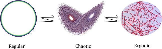
Figure 1. Possible pathway to ergodicity via chaotic dynamics. |
Here, we examine the transition from periodic and quasiperiodic to chaotic orbits through the perspective of position and momentum density distributions and their recurrence plots across different systems, including the harmonic oscillator, the linear and nonlinear Mathieu models, the Lorenz model, and the Nosé–Hoover model. Using these concrete models, we can explore their differences. Our major observations are that while systems with periodic or quasiperiodic trajectories exhibit divergent peaks in their density distributions, followed by periodic or almost semi-periodic recurrence plots (with discontinuous equidistant lines), in some chaotic systems, such as the Lorenz model, the density distribution peaks are smoothed out, leading to a checkboard-like structure of the recurrence plot. Strikingly, we found that not all chaotic systems exhibit this feature. In the Nosé–Hoover model, despite its chaotic nature, the recurrence plot maintains a pattern similar to that seen in quasiperiodic systems. This suggests that while chaotic dynamics can potentially lead to ergodic behavior, it is not sufficient on its own for thermalization and ergodicity. As discussed in [17], ergodicity is achieved only when the system is sufficiently large [14–16].
We explore these models for two basic reasons. First, they can be realized in experimental settings, allowing for precise tuning of all relevant parameters. This high level possibility of control enables us to validate theoretical predictions and observe dynamical behavior directly. Second, these models serve as an excellent starting point for exploring evidence of ergodicity [18]. In large systems, the large number of degree of freedom often complicates their experimental determination [11–13], making the direct verification of the pathway to ergodicity challenging. In these regards, these simple models are valuable for uncovering the fundamental insights into the ergodic behavior before tackling more complicated systems. We hope these results can provide some insight into the intricate relation between chaotic dynamics and ergodicity [2].
(I) Our basic strategy is to explore the dynamics from simple models to nonlinear chaotic models. To address the pathway to ergodicity and to obtain a basic understanding of them, we start from the simple harmonic oscillator
$\begin{eqnarray}\ddot{x}+{\omega }^{2}x=0,\end{eqnarray}$
where x is the position (mass of the pendulum m = 1) and ω is the angular frequency. This equation typically exhibits periodic motion with a closed orbit in the phase space. The solution can be written as $x(t)=R\cos (\omega t+\theta )$. The distribution function, concerning its conservation of energy, is given by $\begin{eqnarray}\rho (x,p)=\delta ({p}^{2}/2+{\omega }^{2}{x}^{2}/2-E),\,\,E\gt 0.\end{eqnarray}$
Obviously, we have ∫ρ(x, p)dxdp = 1. This is a typical result of micro-ensembles in statistical physics. By integrating over the degree of momentum and position, we can obtain the marginal distribution functions as $\begin{eqnarray}P(x)=\int \rho (x,p){\rm{d}}p,\,\,P(p)=\int \rho (x,p){\rm{d}}x.\end{eqnarray}$
The results are given by $\begin{eqnarray}\begin{array}{rcl}P(x) & = & \frac{1}{\sqrt{2E-{\omega }^{2}{x}^{2}}},\,\,| x| \leqslant \sqrt{\frac{2E}{{\omega }^{2}}},\\ P(p) & = & \frac{1}{\omega \sqrt{2E-{p}^{2}}},\,\,| p| \leqslant \sqrt{2E}.\end{array}\end{eqnarray}$
The position and momentum are rescaled via [19]: $\begin{eqnarray}\tilde{x}=-1+\frac{2(x-{x}_{\,\rm{min}\,})}{{x}_{\rm{max}\,}-{x}_{\,\rm{min}}},\,\,\tilde{p}=-1+\frac{2(p-{p}_{\,\rm{min}\,})}{{p}_{\rm{max}\,}-{p}_{\,\rm{min}}},\end{eqnarray}$
where min and max represent the minimal and maximum values of both the position and momentum. respectively. The typical solution of this model and the corresponding closed orbit are presented in figures 2(a) and (b), and their marginal distributions, exhibiting divergent peaks at two magic points, are presented in figures 2(c) and (d). We have verified that the similar magic points can happen in some other (nonlinear) models with periodic orbits, thus this should be a general feature in models with closed orbits. These divergent peaks have an close relation to the the Van Hove singularity in solid materials [20].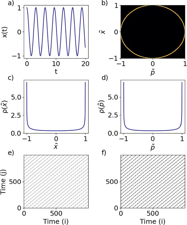
Figure 2. Harmonic oscillator trajectories. (a)–(d) represent the time evolution dynamics, the normalized phase space evolution, and the normalized density distributions, respectively. The parameters are ω = 2, and (x0 = 1, v0 = 0). (e)–(f) represent the recurrence plots for ε = 0.05 and ε = 0.2, respectively. |
This periodic motion means that the system will revisiting the same points over time, which can be perfectly captured by the recurrence plot. Let us define the position in discrete times as ${{\boldsymbol{r}}}_{i}=({\tilde{x}}_{i},{\tilde{p}}_{i})$ (i = 1, 2, 3, ⋯ ), and then define the following recurrence matrix
$\begin{eqnarray}{R}_{ij}=\left\{\begin{array}{ll}1,\quad & | {{\boldsymbol{r}}}_{i}-{{\boldsymbol{r}}}_{j}| \leqslant \epsilon ,\\ 0,\quad & | {{\boldsymbol{r}}}_{i}-{{\boldsymbol{r}}}_{j}| \gt \epsilon ,\end{array}\right.\end{eqnarray}$
where ε is a cutoff. The results for the periodic orbits with different ε are presented in figures 2(e) and (f), showing perfect equidistant diagonal lines, which is a typical feature of periodic orbits. Let us define $\begin{eqnarray}{{\boldsymbol{r}}}_{i}=R\left(\cos (\omega \delta ti),-\omega \sin (\omega \delta ti)\right),\end{eqnarray}$
then the distance Rij = 0 can be reached when and only when ωδt(i − j) = 2πn, $n\in {\mathbb{Z}}$. Hereafter, the diagonal line with i = j will be named as the identity line. In the simulation, we have chosen ω = 2 and δt = 0.01. However, it should be mentioned that for these systems, choosing ε too small may fail to highlight the underlying structure.Periodic systems, by their definition, will never reach a thermal equilibrium because thermalization implies that the system explores all accessible microstates [21, 22], in which the time average will equal the ensemble average given by equation (1 ). In this case, the probability of distribution should be equal to $P(x,p)=(1/Z){{\rm{e}}}^{-\beta V(x)-\beta m{p}^{2}/2}$, where it would be impossible to have sharp peaks. In other words, we can characterize the pathway to ergodicity using these distribution functions and recurrence plots, which is the major theoretical idea used in this work.
(II) We next move to a model that is a little more complicated than the above one by considering the linear Mathieu equation [23, 24]
$\begin{eqnarray}\ddot{x}+(a-2q\cos (2t))x=0,\end{eqnarray}$
which is a second-order differential equation with period T = π. Here a controls the system’s frequency and q the amplitude of the perturbation [24–26]. Stability chart visualizes stable and unstable regions in the (a, q) space can be found in literature [27–31]. We now analyze the resulting phase space density distributions in figure 3. The Mathieu equation exhibits a quasiperiodic behavior under certain conditions, which is reflected in the structure of the phase space and its density distribution. The quasiperiodicity arises from the interaction between the driving force $2q\cos (2t)$ and the system’s intrinsic frequency $\sqrt{a}$. The phase space density shows a concentration of trajectories near extrema, indicating stable and regular oscillations. The corresponding peaks in the marginal distributions of $\rho (\tilde{x})$ and $\rho (\tilde{p})$ reflect the multiple revisiting of some specific points in the phase space showcasing a lack of chaos and a contrast from the uniform characteristics of thermalization. Thus, this trajectory is not ergodic and does not reach thermalization equilibrium.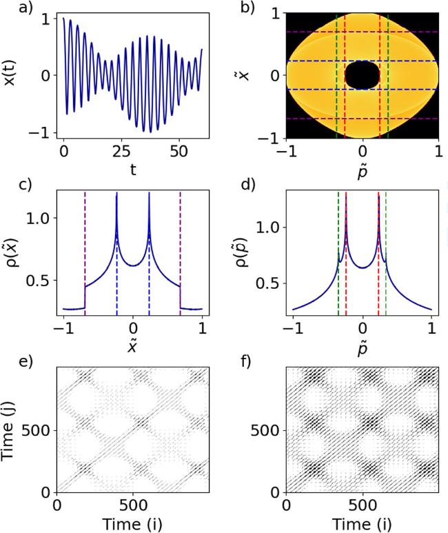
Figure 3. Mathieu linear equation trajectories. (a)–(d)'s details are the same as figure 2, however the parameters are a = 5, q = 1.7, and (x0 = 1, v0 = 0). (e)–(f) represent the recurrence plots for ε = 0.05 and ε = 0.2, respectively. |
For this reason, the recurrence plots in (e) and (f) of figure 3 will exhibit a similar pattern as that in figure 2, using the definition in equation (7 ). However, the diagonal lines become interrupted instead of continuous, signifying that the system is no longer perfectly periodic but quasi-periodic. The quasiperiodicity arises as the system revisits similar states at non-equidistant time intervals. As the system evolves, the phase space orbits reveal two intertwined structures: a smaller orbit (contained between the purple dashed lines) within a larger orbit, as seen in (b). The recurrence plot captures transitions between these two orbits over time, highlighting the complexity of the linear Mathieu equation and explains the quasi-periodic behavior.
(III) The nonlinear Mathieu model may lead to much more complicated dynamics, which are defined as [32, 33]
$\begin{eqnarray}\ddot{x}+(a-2q\cos (2t))x+\eta {x}^{3}=0.\end{eqnarray}$
Depending on the values of these parameters, the nonlinear Mathieu equation can have different behaviors, which is slightly different from the chaotic dynamics. Unlike the linear case, the nonlinearity through η leads to more complicated, irregular behaviors in the phase space and the associated density distributions. The motion in figure 4 shows quasiperiodic oscillations indicating the system’s irregular, yet bounded nature, with a > 0. In this case, the density distributions can still yield divergent peaks. This behavior is still quasi-periodic, thus the recurrence plot is similar to that in figures 3(e) and (f), which also shows interrupted diagonal lines, confirming that the system remains quasi-periodic. However, the phase space trajectories exhibit thinner orbits, corresponding to a decrease in the hollow regions within the recurrence plot. This evolution reflects how the nonlinearity affects the system, tightening the diagonal structure in the recurrence plot and amplifying the sensitivity of the system to parameter changes.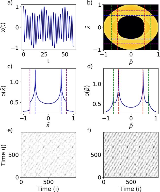
Figure 4. Nonlinear Mathieu equation trajectories. (a)–(d)'s details are the same as figure 2. The parameters are a = 5, q = 1.7, η = 1 and (x0 = 1, v0 = 0). (e)–(f) represent the recurrence plots for ε = 0.05 and ε = 0.2, respectively. |
When a < 0, bifurcations and bistability will be present, leading to some different dynamics. In figure 5 (a), the system oscillates between two extrema, resulting in irregular time evolution, and figure 5(b) reveals that while the system does not have closed or quasiperiodic orbits in the phase space, the trajectories are spread out, occupying a large portion of the phase space. The density distributions in figures 5(c) and (d) do not show divergent peak structures any more, unlike the concentrated peaks seen in previous models. Additionally, instead of a thin closed orbit seen in the Harmonic oscillator, in the nonlinear bistable Mathieu model, the density distribution explores a much broader range of the phase space, leading to a more uniform distribution resembling that of thermalization.
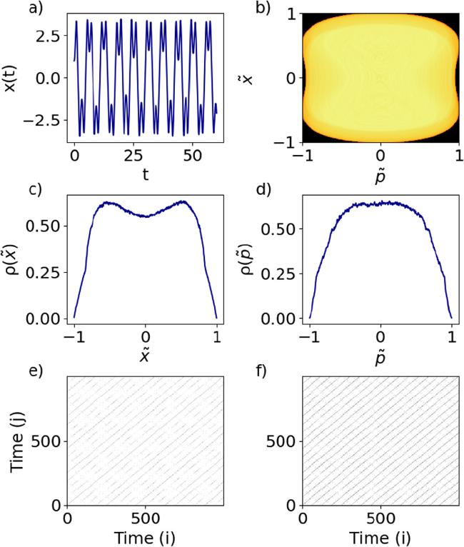
Figure 5. Nonlinear Mathieu equation trajectories. (a)-(d)'s details are the same as figure 2. The parameters are a = − 5, q = 1.7, η = 1 and (x0 = 1, v0 = 0). (e)-(f) represent the recurrence plots for ε = 0.2 and ε = 0.6, respectively. |
In this case the recurrence plot becomes more complex. Now, the diagonal lines include a mix of continuous and interrupted patterns, signifying the emergence of bistability. This comes from the system oscillating between two stable states, depending on the initial conditions and parametric modulation. The recurrence plot captures the interplay between the two stable states, where the diagonal lines represent oscillations within each state. In the phase space, this dynamic is reflected by the disappearance of well-defined orbits, indicating that the system has the tendency of transition into a bounded chaotic regime.
(IV) The previous systems may show that irregularity and non-periodicity are a key to thermalization. Therefore, next we explore the density distribution in the nonlinear Lorenz model [34], which is one of the most famous examples of chaotic dynamics. The Lorenz attractor, discovered by Edward Lorenz in 1963 while investigating atmospheric convection [35], revealed the profound and unexpected nature of deterministic chaos [36, 37]. This discovery marked a significant event in the understanding of complicated physics systems, demonstrating that deterministic equations can produce highly unpredictable and seemingly random behaviors [38–40]. The Lorenz attractor is governed by the following set of ordinary differential equations [41]
$\begin{eqnarray}\left\{\begin{array}{l}\dot{x}=\sigma \left(y-x\right),\\ \dot{y}=x\left(\rho -z\right)-y,\\ \dot{z}=xy-\beta z,\end{array}\right.\end{eqnarray}$
where x, y, and z are state variables and σ, ρ, and β represent the Prandtl number, Rayleigh number, and a geometric factor, respectively [34]. Despite being deterministic, the system exhibits complicated behaviors for certain parameter values [42], in which the transition from regular dynamics to chaotic behaviors, marked by bifurcation points, reveal the system’s rich dynamics [43], offering insights applicable to other chaotic systems [44]. Unlike the harmonic oscillator, the Lorenz model produces chaotic trajectories sensitive to initial conditions [45, 46]. Figures 6(a)–(c) show the Lorenz attractor’s trajectories, illustrating the system’s complicated dynamics in the phase space by defining ${p}_{x}=\dot{x}$, ${p}_{y}=\dot{y}$ and ${p}_{z}=\dot{z}$ and (d)–(f) further visualizes normalized density distributions $\rho (\tilde{x})$, $\rho (\tilde{y})$, and $\rho (\tilde{z})$. These fluctuating patterns confirm the chaotic behavior of the Lorenz system. For chaotic systems, the phase space might be fully revisited, approaching ergodicity.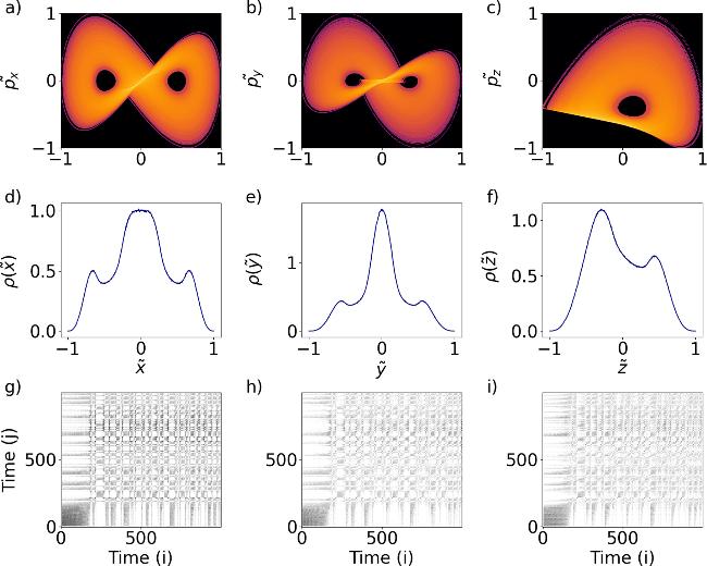
Figure 6. The Normalized Lorenz attractor trajectories projections in the phase space, the normalized density distributions and (g)–(i) are the recurrence plots in the (xy), (xz), and (yz) planes with ε = 0.2. The parameters are σ = 10, ρ = 25, β = 8/3 and the initial conditions (1, 1, 1). |
In figures 6(g)–(i), we plot the recurrence plots in the xy, xz and yz planes, which further illustrates their chaotic dynamics without closed or quasipriodic orbits. In this case, the system has a butterfly-shaped structure in the phase space, characterized by two fixed points. The recurrence plot reflects these dynamics with short diagonal lines and gaps, corresponding to the system’s chaotic transitions between the two fixed points. These transitions are deterministic and unpredictable, leading to the fully chaotic nature of the system. The transitions created in this recurrence plot also indicates the lack of a specific period during the evolution.
(V) Finally, let us consider the Nosé–Hoover model, which is one of the most famous models studied in molecular dynamics for thermalization [17]. The Lorenz model has an intrinsic problem which is that the total volume is not conserved and the trajectories do not satisfy the Liouville law since $V=\partial \dot{x}/\partial x+\partial \dot{y}/\partial y+\partial \dot{z}/\partial z\ne 0$, similar to that in the Lorenz model. The Nosé–Hoover model can be defined by the set of equations [47]
$\begin{eqnarray}\left\{\begin{array}{l}\dot{x}=y,\\ \dot{y}=-x+yz,\\ \dot{z}=1-{y}^{2}.\end{array}\right.\end{eqnarray}$
This model is sensitive to initial conditions similar to the Lorenz model, characteristic of chaotic systems [48]. Ergodicity can be achieved under certain conditions, allowing the system to fully explore its phase space and exhibit equilibrium behaviors. The density distributions of this model have been a zone of interest throughout history in molecular simulations [49]. Figure 7 shows the chaotic behavior of this system, with features similar to that of the Lorenz model and the nonlinear Mathieu equation with bistability. The results demonstrate that in the long time limit the system will visit a large fraction of the phase space. On the other hand, the sharp peaks in the marginal distributions indicate stable configurations, where the system consistently occupies certain positions in the parameter space.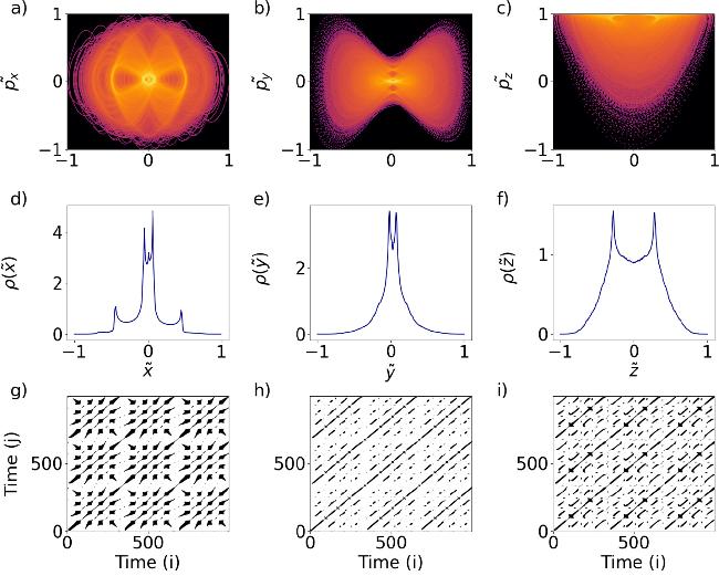
Figure 7. The normalized Nosé–Hoover trajectories projections in the phase space with the initial conditions (0, 5, 0), the normalized density distributions and (g)–(i) are the recurrence plots in the (xy), (xz), and (yz) planes with ε = 0.2. |
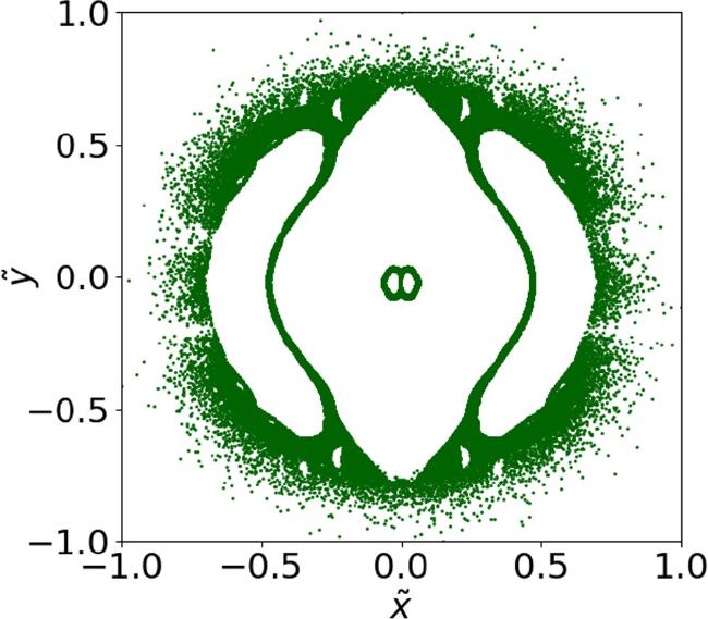
In figures 7(g) to (i), we present the recurrence plots, showing the chaotic dynamics from the Poincaré cross section in figure 8. While this model is believed to be chaotic, its recurrence plots differs significantly from that of the Lorenz attractor. In figure 7, the recurrence plots appear as a uniform pattern of dense dots, indicative of a bounded attractor in the phase space. The dense and uniform structure arises because the system’s dynamics are confined to a tightly bounded trajectory, leading to frequent recurrences within a smaller region of the phase space. This contrasts with the more spread out transitions seen in the Lorenz attractor, highlighting the Nosé–Hoover system’s distinct chaotic behavior. This result indicates that the chaotic dynamics are just one aspect of the Nosé–Hoover model, while another key aspect is its quasi-periodic-like behavior, which leads to the emergence of peaks in the distribution function and discontinuous lines in the recurrence plots.
Discussion and conclusions
While thermalization is often associated with systems containing a large number of particles (N → ∞) [14–16], it can also occur in smaller systems through specific mechanisms. In chaotic dynamical systems, the sensitivity to initial conditions causes trajectories in the phase space to explore more states. As compared with the Lorenz model, the Nosé–Hoover model does not contain fixed points, enabling the system to explore much broader regimes in the phase space, which is necessary to ergodicity. Our findings indicate that, in addition to the well-studied marginal distributions of position and momentum and their comparisons with recurrence plots, there is scope to investigate the potential relationship between ergodicity and chaotic dynamics in small systems. While chaotic dynamics can arise in simple models without thermalization, their trajectories often traverse large regions of the phase space, displaying features that resemble ergodicity. The results presented in this work fully agree with this point from the perspective of distribution and recurrence plots. As discussed in the original manuscript by Hoover [17], in small systems like the model in model (V), the trajectory may visit a larger portion of the phase space due to the chaotic nature of the system (see [47]). This is demonstrated by the Poincaré cross section in figure 8. In molecular simulations, ergodicity and thermalization are typically achieved only when the number of atoms is sufficiently large, facilitated by chaotic dynamics. With the breakdown of solvability due to nonlinear interactions, these systems can evolve into chaotic dynamics, offering a plausible pathway to thermalization. While chaotic dynamics in small systems may not fully realize this process, they exhibit a clear tendency toward this goal.
Figure 8. The Poincaré plot at z = 0 for the chaotic dynamics of the Nosé–Hoover model. |
In this work, the nature of the density distribution in phase space provides key insights into a system’s ergodicity. In chaotic and bistable systems, the disappearance of divergent peaks and the emergence of a Gaussian-like distribution indicate ergodicity, where the system explores the entire phase space weighted by a Gaussian function. This behavior reflects the system’s ability to visit a wide range of states without being confined to specific trajectories. In contrast, periodic or quasi-periodic systems display non-ergodic behavior, characterized by divergent peaks and localized density distributions. Here, certain points in phase space are revisited frequently, while others remain unexplored, highlighting their structured and constrained dynamics. Thus, the form of the density distribution serves as a distinguishing factor between chaotic or bistable (ergodic) systems and periodic or quasi-periodic (non-ergodic) systems. Due to their simplicity, these models are well-suited for illustrating the primary pathways to thermalization in small systems. They can be directly implemented in experiments, such as trapped-ion quantum simulators [50], three superconducting qubits [51], and two-dimensional photon gases in optical microresonators [52], providing valuable insights into thermalization processes. However, the fundamental principles of ergodicity in statistical mechanics can only be fully realized in the large N limit. The key takeaway is that while chaotic dynamics offer the most plausible pathway to thermalization, small systems cannot fully achieve ergodicity. Furthermore, small chaotic models may exhibit dynamics resembling quasi-periodic systems, suggesting that ergodicity through chaotic dynamics is feasible only in larger systems. Therefore, system size must be considered a critical parameter when discussing ergodicity. Finally, it should be noticed that this pathway is by no means simple and straightforward, since the many-body dynamics may also contain limit cycles, leading to some intriguingly dynamics not discussed in this work [53].