


1. Introduction
Magnetic ordering mediated by itinerant electrons is a fundamental subject with a long history in the study of correlated materials. Early prominent examples where this mechanism is at play include rare-earth compounds [1] and heavy-fermion systems [2, 3], which are still at the forefront of condensed matter physics, due to their rich collective behaviors. The indirect coupling between localized spins can be understood to arise from the Ruderman-Kittel-Kasuya-Yosida (RKKY) interaction [4–7] and, depending on the electronic band structure and exchange coupling strength, a wide variety of magnetic transitions may be observed.
Recent interest in this physics has also arisen in engineered nanostructures with reduced dimensions, such as one-dimensional (1D) chains of magnetic atoms deposited on metallic surfaces [8] or nuclear spins in nanotubes and nanowires, which might enter a helical phase at sufficiently low temperatures [9–11]. Atomic chains, in particular, offer considerable flexibility in tailoring magnetic interactions. Besides conventional ferromagnetic and antiferromagnetic states [12–16], more complex types of noncollinear order, such as spiral configurations [17–19], have been realized. In proximity to conventional s-wave superconductors, these magnetic chains have also emerged as a promising experimental platform for topological superconductivity [19–21]. In this context, self-organized spiral order could naturally stabilize a topological phase hosting Majorana edge states, without requiring fine-tuning external parameters [22–24]. In spintronic devices, spiral order may be exploited for spin and charge pumping, by inducing a rotational motion of the spin texture analogous to an Archimedean screw [25–27].
The Kondo lattice model represents an established paradigm to describe these systems, when the overlap between itinerant electrons and localized magnetic moments dominates over direct spin-spin interactions. The properties of the 1D Kondo lattice have been extensively investigated over the years [28, 29], showing that the general case with quantum localized spins gives rise to rich correlation effects and phase diagrams [29]. More recently, the surge of interest in topological superconductivity has brought renewed attention to this model, with the localized spins treated classically [30–33]. Based on an explicit ansatz, a competition between spiral order and ferromagnetic/antiferromagnetic states has been revealed [30, 31]. Monte Carlo simulations find additional phases, with complex collinear and noncollinear textures [32, 33].
The intricacies of the phase diagram have motivated us to study the problem with an alternative approach, based on a recent analysis of the dissipative dynamics in the presence of an applied voltage bias [27]. The equilibrium limit of that treatment yields a set of dynamical equations that relax the system to a stationary magnetic configuration. We have performed a comprehensive analysis of these low-energy states and determined how they affect the phase diagram. The result is surprising, given that previous studies always find an extensive region of spiral order [30–33]. Here we show, instead, that it is always possible to relax the spiral states to a more favorable noncollinear configuration. The free energy difference persists in the thermodynamic limit, where we also find that the magnetic texture maintains a finite deviation from the original spiral. The new state is actually a modulated spiral, where the modulation wavelength is determined by the Fermi wavevector of the unperturbed spiral state. Therefore, we interpret the appearance of complex noncollinear order as due to an instability of the spiral states. This general mechanism is consistent with our findings that spiral order is never a locally stable magnetic state. Although the modulation can also reach a large amplitude, there are certain regimes in which it becomes a weak perturbation of the harmonic spiral. In particular, at small exchange coupling J, the gain in free energy vanishes as ΔF ∼ J4, which might explain why complex noncollinear states were previously missed.
The paper is structured as follows: In section 2 , we introduce the model under study, and in section 3 , we perform a preliminary analysis based on trial states. Section 4 describes the dissipative dynamics adopted in this work. Based on this approach, in section 5 , we characterize the noncollinear states in terms of a modulated spiral order and discuss our final phase diagram. In section 6 , we present our conclusions and an outlook for future research.
2. Model
The system under study is described by the 1D Kondo lattice model [28, 29]: 1 ), throughout this study we will impose periodic boundary conditions.
$\begin{eqnarray}H=-w\displaystyle \sum _{i,\sigma }({c}_{i\sigma }^{\dagger }{c}_{i+1\sigma }+{\rm{H.c.}})-\mu \displaystyle \sum _{i,\sigma }{c}_{i\sigma }^{\dagger }{c}_{i\sigma }+2J\displaystyle \sum _{i}{{\boldsymbol{m}}}_{i}\cdot {{\boldsymbol{s}}}_{i},\end{eqnarray}$
where mi are classical Heisenberg spins, which we take as normalized (∣mi∣ = 1). The itinerant electrons are described by a tight-binding Hamiltonian with nearest-neighbor hopping amplitude w and chemical potential μ. The fermionic creation operators are ${c}_{i\sigma }^{\dagger }$, where i = 1, 2, …, L is the lattice site and σ = ↑ , ↓ the spin index. The magnetic interaction between the localized spins and the electronic spin polarization ${{\boldsymbol{s}}}_{i}=\frac{1}{2}{\sum }_{\sigma ,{\sigma }^{{\prime} }}{{\boldsymbol{\sigma }}}_{\sigma {\sigma }^{{\prime} }}{c}_{i\sigma }^{\dagger }{c}_{i{\sigma }^{{\prime} }}$ (where σ is the vector of Pauli matrices) is controlled by the on-site exchange coupling J. Note that, as indicated in equation (The above Hamiltonian models the interplay between itinerant electrons and a lattice of localized classical Heisenberg spins, where the indirect exchange interaction mediated by the electrons gives rise to various types of magnetic order. For a given configuration of the classical spins mi, the Hamiltonian can be readily diagonalized in real space. In terms of the 2L fermionic eigenmodes aα = ∑i,σUα;iσciσ, where Uα;iσ = ⟨α∣iσ⟩ is the appropriate unitary matrix, H reads: 2 ) and (3 ) are relatively straightforward to compute numerically, one is then faced with the problem of finding the energetically favored configuration of the classical spins. The mi determines the single-particle eigenvalues εα in a nontrivial way, thus, the problem of minimizing F is computationally challenging. In particular, we are interested in finding the magnetic state in the thermodynamic limit, when the number of spin directions mi to optimize diverges with system size. The problem has been approached with classical Monte Carlo methods, giving somewhat conflicting results for the phase diagram [32, 33]. In the following, we will tackle the minimization problem by evolving the system under a suitable dissipative dynamics. This approach is suggested by a recent study of the driven-dissipative nonlinear dynamics of equation (1 ), induced by applying an external voltage bias [27]. As it turns out, the equilibrium limit of that treatment provides us with an effective method to characterize the ground state.
$\begin{eqnarray}H=\displaystyle \sum _{\alpha =1}^{2L}\left({\epsilon }_{\alpha }-\mu \right){a}_{\alpha }^{\dagger }{a}_{\alpha }.\end{eqnarray}$
In this article, we will restrict ourselves to the limit of zero temperature. Therefore, the free energy per site is simply obtained as: $\begin{eqnarray}F=-\frac{1}{L}\displaystyle \sum _{\alpha =1}^{2L}(\mu -{\epsilon }_{\alpha })\theta (\mu -{\epsilon }_{\alpha }),\end{eqnarray}$
where θ(ε) is the Heaviside step function. While the above equations (In concluding this section, we note that, for classical Heisenberg spins, the sign of J is not important. The ground state with an opposite value of the exchange coupling, J → − J, is obtained by flipping the magnetic configuration, mi → −mi. Furthermore, it is easily seen that a particle-hole transformation of equation (1 ) leads to w → −w, J → −J, and μ → −μ. However, the sign of the hopping amplitude is also unimportant. It can be changed by the unitary transformation ciσ → (−1)iciσ if L is even and, in the thermodynamic limit, the parity of L has no influence on the properties of the system. Therefore, we can always restrict ourselves to positive values of w, J, and μ. Note that our choice of a positive μ corresponds to an electronic occupation which, for J → 0, is larger than half-filling. The states below half-filling are described by negative values of μ, and their ground state is obtained by flipping the magnetic configuration: Setting μ →−μ at given values of w and J implies mi → −mi.
3. Competition of spiral and collinear order
We first analyze the system within the following spiral ansatz: 4 ) has been analyzed by [30] for electrons in a continuum, and by [31] for the same tight-binding model of equation (1 ). The phase diagram also includes ferromagnetic and antiferromagnetic states, which can be simply obtained from equation (4 ) by setting qs = 0 and qs = π, respectively. As we will see below, more general collinear and noncollinear states are often favored. However, a large region of spiral order survives in the phase diagrams of [32, 33], where unrestricted spin configurations were studied with Monte Carlo techniques.
$\begin{eqnarray}{{\boldsymbol{m}}}_{i}=(\cos ({q}_{s}i),\sin ({q}_{s}i),0),\end{eqnarray}$
which is schematically presented in figure 1(a) and has been suggested as the appropriate magnetic state at small values of J. In this limit, according to the RKKY mechanism, the ground state configuration favors the appearance of spiral order [9, 10, 29–33]. This spiral state can be understood to arise from a spin-selective Peierls instability [34] and, due to the half-gapped energy dispersion of its electronic bands, results in a reduction of electric conductance by a factor of two [9–11]. Beyond the RKKY limit, the spiral ansatz of equation (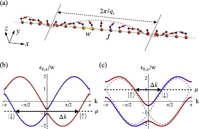
Figure 1. (a) Schematic representation of spiral order in the 1D Kondo lattice model. (b) Dispersion of the electronic states, given by equation ( |
The spiral state is most easily analyzed by applying the gauge transformation ${c}_{j\uparrow }^{\dagger }\to {\rm{e}\,}^{\,\rm{i}{q}_{s}j/2}{c}_{j\uparrow }^{\dagger }$ and ${c}_{j\downarrow }^{\dagger }\to {\rm{e}\,}^{-\,\rm{i}{q}_{s}j/2}{c}_{j\downarrow }^{\dagger }$, which is designed to transform the spin configuration to the transitionally invariant state mi = (1, 0, 0). At the same time, spin–orbit coupling is introduced in the electronic Hamiltonian [30, 31, 34, 35]. In the transformed frame, the eigenstates have a definite wavevector k ∈ [− π, π] and their energy dispersion can be readily derived as: 3 ) as: 5 ), computed at the appropriate values of qs = qopt. As seen, the exchange interaction leads to the opening of a partial gap at the Fermi energy, while one of the bands remains partly occupied. We denote by Δk the difference between the two Fermi wavevectors of the spiral state, which will play an important role later on.
$\begin{eqnarray}{\epsilon }_{k,\pm }=-2w\cos k\cos \frac{{q}_{s}}{2}\pm \sqrt{{J}^{2}+4{w}^{2}{\sin }^{2}k{\sin }^{2}\frac{{q}_{s}}{2}}.\end{eqnarray}$
The free energy is immediately obtained from equation ( $\begin{eqnarray}{F}_{s}=-\displaystyle \sum _{\sigma =\pm }{\int }_{-\pi }^{\pi }\frac{\,\rm{d}\,k}{2\pi }\left(\mu -{\epsilon }_{k,\sigma }\right)\theta \left(\mu -{\epsilon }_{k,\sigma }\right).\end{eqnarray}$
Finally, the optimal spiral can be found by minimizing the free energy Fs over qs. In the J ∼ 0 limit, the optimal wavevector satisfies qopt ≃ ± 2kF, where the sign determines the chirality of the spiral and ${k}_{F}=\pi -\arccos (\mu /2w)$ is the Fermi wavevector of the unperturbed Fermi gas (i.e., obtained at J = qs = 0). We show in figures 1(b) and (c) representative plots for the dispersion relation of equation (Going beyond equation (4 ), other types of magnetic order were found in certain parts of the phase diagram [32, 33]. Among them, collinear states are the easiest to analyze, and in this work, we have considered arbitrary configurations that can be written in terms of a periodic cell with up to six lattice sites. For example, a cell with one site gives the ferromagnetic state ↑, and a cell with two sites gives the antiferromagnetic state ↑ ↓ . Larger unit cells lead to more complex collinear configurations, among which the one that features more prominently in the phase diagram is ↑ ↑ ↓ ↓ [32]. Because of their periodic structure, the free energy of the infinite system can be obtained easily. However, we find it more convenient to rely on equation (3 ), considering sufficiently large values of L at which finite-size effects become negligible. In practice, we compute the free energy of the collinear states using L = 1000 if the unit cell has four or five sites, and L = 1002 if the unit cell has three or six sites (to guarantee the periodic boundary condition). We construct the phase diagram by considering a grid of values with Δμ = ΔJ = 0.04w, which we will also use for the unrestricted phase diagram. At each value of μ and J, we compare the free energy of the optimal spiral state (qs = qopt) with that of the aforementioned collinear states, obtaining the result shown in figure 2(a).
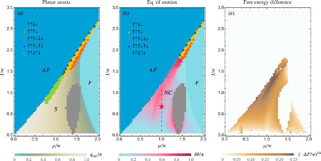
Figure 2. (a) Ansatz-based phase diagram, including the spiral states of equation ( |
This ansatz-based phase diagram exhibits several notable features. First, the spiral (S), ferromagnetic (F), and antiferromagnetic (AF) phases described by equation (4 ) occupy the largest portion of the phase diagram [30, 31]. However, we also identify five collinear magnetic states with lower free energy than the spiral ansatz. There is a continuous transition between the spiral and ferromagnetic phases [30, 31], while all other phase transitions are first-order. Among the nontrivial collinear states, ↑ ↑ ↓ ↓ is favored at infinitesimally small values of the exchange coupling J when $\mu /w=\sqrt{2}$, signaling a breakdown of the perturbative RKKY mechanism [32]. This phase occupies a relatively large region, extending up to intermediate values of J ∼ 1.2w, while other collinear magnetic states only appear in a narrow strip close to the AF phase. These results are in good agreement with [32, 33], which both find the existence of a narrow region of ↑ ↑ ↑ ↓ ↓ ↓ order. The phase diagram of [33], however, appears to be more accurate. It also finds a ↑ ↑ ↑ ↓ phase, which is confirmed by our figure 2(a). Additionally, an extremely thin region with the complex collinear state ↑ ↑ ↑ ↓ ↑ ↓ ↓ ↓ ↑ ↓ appears in [33] at the boundary with AF. In our calculations, we also have indications of the existence of an additional phase, since the somewhat related state ↑ ↑ ↑ ↓ ↑ ↓ appears at selected cells along the AF boundary. However, our grid is too coarse to resolve this region accurately and in any case, we have only considered unit cells with up to six sites. Following [33], ↑ ↑ ↑ ↓ ↑ ↓ is likely a spurious phase.
Instead, the most important shortcoming of figure 2(a) is the absence of complex noncollinear order, i.e., noncollinear states beyond equation (4 ). Both [32] and [33] agree on this point, although in the former case the additional phase is denoted as ‘noncoplanar’, while the latter study finds ‘complex noncollinear structures’ which are always planar. Part of the ↑ ↑ ↑ ↓ ↓ ↓ , ↑ ↑ ↑ ↓ , and S phases, as well as the whole ↑ ↑ ↓ ↑ ↓ region, would be occupied by this new phase. These findings, and the disagreements regarding the precise form of the complex noncollinear states, motivate us to analyze the problem with an alternative approach.
In this work, we rely on a dissipative evolution introduced by our recent study of a voltage-biased Kondo chain [27]. Considering such evolution in the equilibrium limit makes the spiral state naturally relax towards a more complex noncollinear state, which is a local minimum of the free energy. Doing so, we will obtain our final phase diagram, presented in figure 2(b). As shown in figure 2(c), where the free energy difference between the states of panels (b) and (a) is computed explicitly, this method allows us to improve the magnetic configuration. In figure 2(c), there is a large region of negative values, corresponding to noncollinear magnetic configurations different from the spiral ansatz.
4. Equation of motion approach
The equations of motion adopted here are valid for a sufficiently slow spin dynamics, which allows us to assume that, for a given configuration of classical spins, the electrons instantaneously reach their steady state. This approach effectively separates the degrees of freedom into fast-moving conduction electrons and slow-moving classical spins, and is completely analogous to the familiar Born-Oppenheimer approximation describing the electronic and nuclear motions in molecules and solids. From the instantaneous ground state, we can immediately write the expression of the correlation function ${\chi }_{i,\sigma ;{i}^{{\prime} },{\sigma }^{{\prime} }}=\langle {c}_{i\sigma }{c}_{{i}^{{\prime} }{\sigma }^{{\prime} }}^{\dagger }\rangle $: 2 ), is the unitary matrix bringing H to diagonal form.
$\begin{eqnarray}{\chi }_{i,\sigma ;{i}^{{\prime} },{\sigma }^{{\prime} }}=\displaystyle \sum _{\alpha }{U}_{\alpha ;i\sigma }^{* }{U}_{\alpha ;{i}^{{\prime} }{\sigma }^{{\prime} }}\theta ({\epsilon }_{\alpha }-\mu ),\end{eqnarray}$
where Uα;iσ, defined right above equation (The dynamics of mi under the influence of the exchange field is modeled by a standard Landau–Lifshitz-Gilbert (LLG) equation [27, 36–39]: 8 ) plays the same role as the potential energy surfaces, which determine the equations of motion of the nuclear coordinates. Since $\left\langle {{\boldsymbol{s}}}_{i}\right\rangle $ is generally noncollinear with mi, it gives rise to a nontrivial torque term, proportional to $\left\langle {{\boldsymbol{s}}}_{i}\right\rangle \times {{\boldsymbol{m}}}_{i}$. The resulting dynamics is inherently nonlinear, due to the self-consistent nature of the interaction between the spin configuration and the electronic system. Specifically, the local spin orientations mi determine the electronic correlation function χ, which in turn influences the evolution of mi through the spin polarization $\left\langle {{\boldsymbol{s}}}_{i}\right\rangle $. This feedback loop results in a complex dynamics, driving the system towards a low-energy state.
$\begin{eqnarray}\frac{\partial {{\boldsymbol{m}}}_{i}}{\partial t}=J\left\langle {{\boldsymbol{s}}}_{i}\right\rangle \times {{\boldsymbol{m}}}_{i}+\eta \left(\left\langle {{\boldsymbol{s}}}_{i}\right\rangle \times {{\boldsymbol{m}}}_{i}\right)\times {{\boldsymbol{m}}}_{i},\end{eqnarray}$
where $\begin{eqnarray}\left\langle {{\boldsymbol{s}}}_{i}\right\rangle =\frac{1}{2}\displaystyle \sum _{\sigma ,{\sigma }^{{\prime} }}{{\boldsymbol{\sigma }}}_{\sigma {\sigma }^{{\prime} }}\left\langle {c}_{i\sigma }^{\dagger }{c}_{i{\sigma }^{{\prime} }}\right\rangle =-\frac{1}{2}\displaystyle \sum _{\sigma ,{\sigma }^{{\prime} }}{{\boldsymbol{\sigma }}}_{\sigma {\sigma }^{{\prime} }}{\chi }_{i{\sigma }^{{\prime} },i\sigma }.\end{eqnarray}$
The phenomenological damping rate η describes a relaxation process towards the direction antiparallel to the electronic spin polarization. Returning to our analogy with the Born-Oppenheimer approximation, the exchange field of equation (A representative example of the time evolution, taking the spiral state as initial condition, is shown in figure 3. We have plotted the free energy F and the maximum deviation Θ from mi and $\left\langle {{\boldsymbol{s}}}_{i}\right\rangle $ being antiparallel:
$\begin{eqnarray}{\rm{\Theta }}={{\rm{\max }}}_{i}\left|{\cos }^{-1}\frac{{{\boldsymbol{m}}}_{i}\cdot \,\left\langle \,{\,{\boldsymbol{s}}}_{i}\right\rangle }{\left|\,\left\langle {{\boldsymbol{s}}}_{i}\right\rangle \right|}-\pi \right|.\end{eqnarray}$
We also rely on the spin chirality to characterize the planar nature of the noncollinear phase: $\begin{eqnarray}V={{\rm{\max }}}_{i}\left|\left({{\boldsymbol{m}}}_{i}\times {{\boldsymbol{m}}}_{i+1}\right)\cdot {{\boldsymbol{m}}}_{i+2}\right|.\end{eqnarray}$
As seen in figure 3, the evolution process generally consists of three stages. Initially, the spiral order evolves very slowly and remains nearly stationary. In the second stage, the system undergoes significant changes, with a rapid decrease in free energy and the emergence of noncoplanar spin configurations. Finally, the classical spins relax into a noncollinear stationary state, where the free energy stabilizes and the spins become planar again. In agreement with [33] (and at variance with [32]), we always find that the mi relaxes to a planar configuration. We note, however, that V has a longer relaxation time than F and Θ. Therefore, a planar state is only obtained if the simulation is extended to sufficiently long times.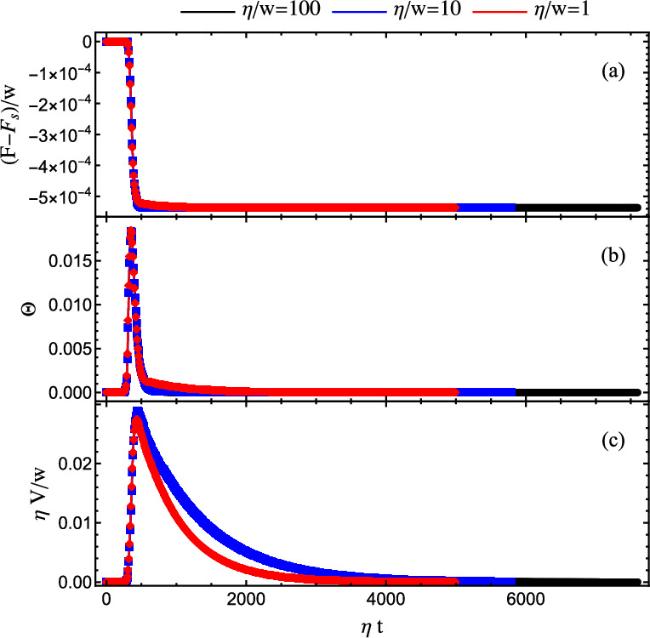
Figure 3. Time evolution starting from a spiral state, using η/w = 1 (red), 10 (blue), and 100 (black). (a) Free energy difference as a function of time. (b) Time dependence of Θ, defined in equation ( |
From the asymptotic time dependence, we extract the stationary value of the free energy: appendix .
$\begin{eqnarray}{F}_{{\rm{eq}}}=\mathop{\mathrm{lim}}\limits_{t\to \infty }F(t)\simeq F({t}_{{\rm{\max }}}),\end{eqnarray}$
where ${t}_{{\rm{\max }}}$ is the numerical cutoff of the simulation. In practice, to obtain figure 2(b) we have used ${t}_{\,\rm{max}\,}\,={\rm{\min }}\left\{{t}_{0},{t}_{1}\right\}$, where t0 = 500w−1 and t1 satisfies: $\begin{eqnarray}\begin{array}{l}\frac{F({t}_{1}-10{w}^{-1})-F({t}_{1})}{F(0)-F({t}_{1})}\\ \quad \lt 1{0}^{-3}\quad {\rm{and}}\quad F(0)-F({t}_{1})\gt 1{0}^{-9}.\end{array}\end{eqnarray}$
It is also worth stressing that Feq is not necessarily the ground-state energy, since we have assumed that the classical spins initially adopt the planar ansatz configuration. This point is discussed explicitly in the Finally, we comment on the different role played by the relaxation rate η in the non-equilibrium evolution of [27] and in the present case. While under an external voltage bias, the asymptotic dynamics of the Kondo chain have a nontrivial character (periodic, quasiperiodic, or chaotic) and depend sensitively on the value of η. This is not the case in equilibrium when, like in figure 3, a stationary configuration is eventually reached. In the stationary state, each mi is antiparallel to the local spin polarization $\left\langle {{\boldsymbol{s}}}_{i}\right\rangle $, as shown by the vanishing value of Θ in figure 3(b). Having antiparallel mi and $\left\langle {{\boldsymbol{s}}}_{i}\right\rangle $ is a necessary condition for the stationary points of the free energy, and ensures that both the torque and damping term of equation (8 ) vanish. This implies that the value of η and the adiabatic approximation should not affect the final equilibrium spin configuration, thus, the relaxation rate η can be chosen freely. This point is demonstrated explicitly in figure 3, obtained by computing the relaxation process with three different values of η. As seen, the features of the asymptotic state (t → ∞) are independent of η. The time evolution is very similar in the three cases, after rescaling the time and the spin chirality V with η. As expected, at larger η, the relaxation to the equilibrium state proceeds faster. Furthermore, panel (c) shows that a larger η also leads to smaller deviations from a planar configuration throughout the whole time evolution. Therefore, in all calculations presented in this study, we have used a large relaxation rate, η = 100w.
5. Analysis of the noncollinear phase
After having established the general framework, we are now ready to present our main results. In the previous section, we have shown that the dissipative evolution of equations (7 )–(9 ) leads to a configuration of the mi with lower energy than the spiral ansatz of equation (4 ). In this section, our first aim will be to establish that the physical differences between these noncollinear states and the spiral ansatz survive in the thermodynamic limit. Furthermore, by examining in more detail the properties of the noncollinear states, we will suggest the physical mechanism behind the deviations from the harmonic spiral. This analysis will support the validity of our phase diagram, which we have already presented in figure 2(b).
5.1. Finite-size scaling
A representative example of the finite-size scaling behavior is shown in figure 4. In the upper panel, we compare the free energy Fs of the optimal spiral state (i.e., with qs = qopt) and Feq, obtained from the evolution of the optimal spirals as in equation (12 ). The dependence of Feq shows more pronounced oscillations, which, as discussed in the appendix , are related to our choice of the initial state. Still, the amplitude of these oscillations decreases with L and is always much smaller than Fs − Feq. The energy difference Fs − Feq remains finite and is approximately constant for L > 600, showing good convergence properties in the limit L → ∞.
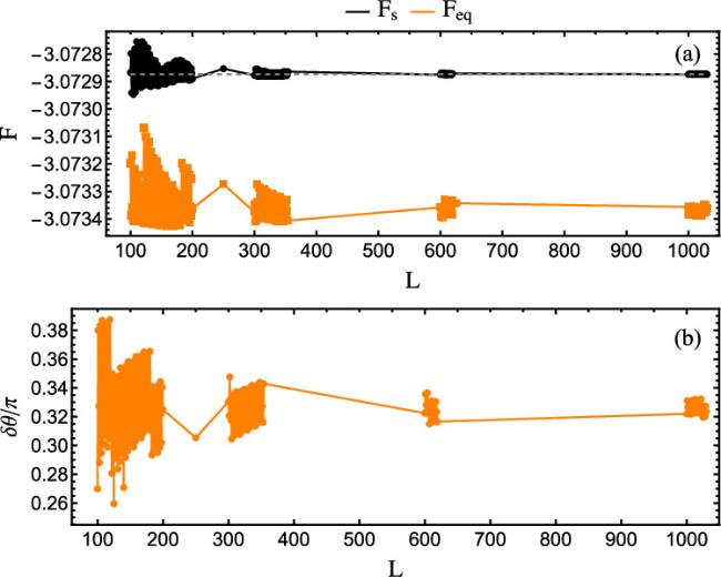
Figure 4. Finite-size scaling of (a) the free energy F and (b) the parameter δθ, defined in equation ( |
Similar considerations hold for δθ, which is a useful characterization of the spin configuration and is plotted in figure 4(b). We define δθ by first writing:
$\begin{eqnarray}{{\boldsymbol{m}}}_{i}=(\cos ({\phi }_{i}),\sin ({\phi }_{i}),0),\end{eqnarray}$
which is allowed by the planar nature of the equilibrium state. Therefore, the magnetic configuration can also be characterized by the sequence of relative angles, θi = φi+1 − φi. More precisely, ${\theta }_{i}=\arccos ({{\boldsymbol{m}}}_{i}\cdot {{\boldsymbol{m}}}_{i+1})\in (-\pi ,\pi ]$, from where we compute: $\begin{eqnarray}\delta \theta ={{\rm{\max }}}_{i}| {\theta }_{i}| -{{\rm{\min }}}_{i}| {\theta }_{i}| .\end{eqnarray}$
The spiral ansatz has a constant relative angle θi = qs, giving δθ = 0. On the other hand, nontrivial forms of collinear order (other than F and AF) yield the maximum value δθ/π = 1. We see that the spin configuration of figure 4(b) converges to an intermediate value δθ/π ≃ 0.32 at large system size, reflecting the presence of a complex noncollinear order.We have checked that a behavior similar to figure 4 is obtained for several other choices of μ and J, indicating that the system size used to derive our phase diagram (L = 1000) is sufficiently large. While figure 2 is representative of the thermodynamic limit, we should also point out that at small values of J, the finite-size scaling becomes more challenging. This will become clear further below, in connection with figure 7, and is related to the fact that for J → 0 the magnetic configuration approaches the spiral ansatz (ΔF, δθ → 0).
5.2. Modulated spiral order
The spatial dependence of the relative angles, plotted in figure 5(a), gives considerable insight into the nature of the noncollinear states. As seen, the modulations of the θi can be accurately described by the following oscillatory dependence: 16 ), qopt is the optimal wavevector of the spiral ansatz. Instead, the amplitude of the oscillation is the parameter defined in equation (15 ). Since 2π/Δk is generally incommensurate with the lattice, in an infinite system, there will be sites which approach θi = qopt ± δθ/2 with arbitrary precision. A similar argument shows that the parameter Φ has no physical significance. By translating the magnetic configuration of an infinite system by ℓ, the phase transforms to Φ + Δk · ℓ, which can assume any arbitrary value. Instead, the most important parameter of equation (16 ) is the wavevector of the periodic modulation, which coincides with the separation Δk between the two Fermi points of the spiral state. The dispersion, together with the definition of Δk, is illustrated in figures 1(b) and (c). This observation reveals that the noncollinear magnetic states arise from an instability of the spiral order, induced by a spontaneous modulation of the classical spin directions. This modulation has periodicity 2π/Δk and induces scattering between the two Fermi points, leading to the formation of a gapped state with lower energy than the harmonic spiral.
$\begin{eqnarray}{\theta }_{i}\simeq {q}_{{\rm{o}}{\rm{p}}{\rm{t}}}+\frac{\delta \theta }{2}\cos ({\rm{\Delta }}k\cdot i+{\rm{\Phi }}),\end{eqnarray}$
which is plotted as a red dashed curve in figure 5(a). In equation (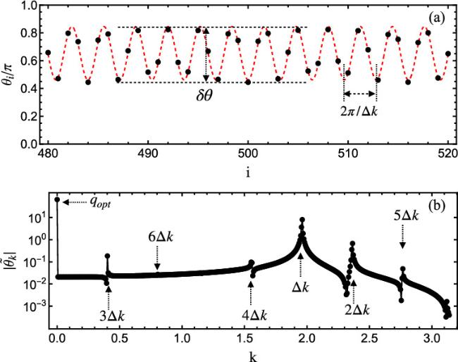
Figure 5. (a) Relative angles of the modulated spiral state. The red dashed line is the fitting curve equation ( |
While equation (16 ) provides a good fit to the numerical results across a broad range of exchange couplings J and chemical potentials μ, we can further analyze the noncollinear states by applying a discrete Fourier transform to the relative angles:
$\begin{eqnarray}{\tilde{\theta }}_{k}=\frac{1}{\sqrt{L}}\displaystyle \sum _{j=1}^{L}{\theta }_{j}{\rm{e}\,}^{\,\rm{i}kj}.\end{eqnarray}$
The Fourier spectrum is presented in figure 5(b), showing that, indeed, the dominant frequency component is at k = Δk. However, there is also a series of peaks at the higher-order harmonics, such as 2Δk, 3Δk, 4Δk… , whose amplitudes decrease with the order of the harmonics. As shown in figure 6, the behavior observed at the specific values of μ and J of figure 5 is, in fact, completely general. By computing the Fourier spectrum along a linecut with μ/w = 1, we are always able to identify all the peaks as due to a modulation with wavevector Δk, together with its higher-order harmonics. The strength of these peaks is shown in figure 6(a). The higher-order peaks become negligible at small J, where a nearly ideal harmonic modulation is realized. Instead, at a large value of J, the periodic dependence becomes anharmonic. Still, the absence of other Fourier components indicates that the modulation is entirely due to an instability of the spiral state at its two Fermi points. Figure 6 also reveals that a finite modulation persists below J ∼ 0.5, where a harmonic spiral is found in the phase diagram of [33]. In fact, from the physical picture suggested here, it is natural to expect that the spiral state will always be subject to an instability. Then, at variance with [32, 33], it will never appear in the phase diagram. As we will describe in more detail below, this is the only essential difference between our phase diagram and [33].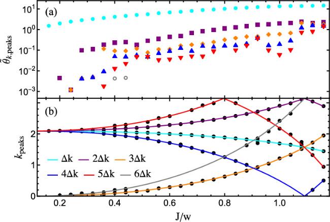
Figure 6. Fourier analysis along the linecut μ/w = 1 of figure 2(b). (a) Value of $| {\tilde{\theta }}_{k}| $ at the local maxima in the Fourier spectrum. (b) Positions of the peaks. The interpolating lines are obtained from equation ( |
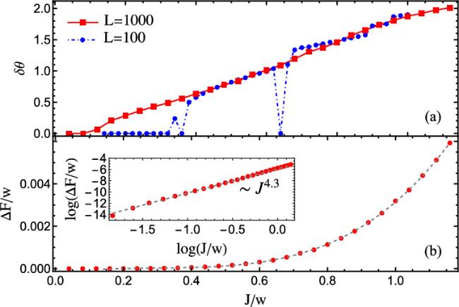
Figure 7. (a) Plot of δθ as a function of exchange coupling J. Blue (dot-dashed) and red (solid) curves are for system sizes L = 100 and L = 1000, respectively. (b) Free energy difference ΔF as a function of J. The inset shows a power-law fit, yielding an exponent of 4.3. Other parameters correspond to the μ/w = 1 linecut of figure 2(b). |
5.3. Phase diagram
We now return to the phase diagram of figure 2(b), which was obtained as a function of μ and J by applying the equation of motion approach to the optimal spiral ansatz. Doing so, we find noncollinear (NC) states with Feq < Fs and, after comparing Feq to the free energy of the same collinear states considered in figure 2(a), we finally obtain figure 2(b). This phase diagram is computed with L = 1000, but as we have already discussed, the system size is sufficiently large to describe the thermodynamic limit.
Compared to figure 2(a), the S phase is replaced now by a NC region which, as expected, occupies a larger portion of the phase diagram. The ↑ ↑ ↓ ↓ phase shrinks slightly, the ↑ ↑ ↓ ↑ ↓ phase disappears, and the other collinear magnetic phases are significantly reduced. The color gradient in the NC region of figure 2(b) indicates the value of δθ, which is generally finite but can become small in certain regimes. In particular, δθ → 0 if J → 0 and when approaching the F phase. In the same limits, we also obtain a vanishing difference of the free energy, ΔF → 0, shown in figure 2(c). At the boundary with the F phase, the vanishing of δθ and ΔF indicates a continuous NC–F transition, analogous to the S–F transition of figure 2(a). Instead, all other phase transitions in figure 2(b) are first-order.
Compared to [32] and [33], where the Monte-Carlo method was employed, our approach explicitly identifies a generic breakdown of the harmonic spiral. Otherwise, our figure 2(b) is in good agreement with figure 2 of [33]. In particular, their H phase (indicating a complex noncollinear order) has a good overlap with the region of our figure 2(b) where δθ ≳ 0.5. Furthermore, the competition between noncollinear states and the ↑ ↑ ↑ ↓ , ↑ ↑ ↑ ↓ ↓ ↓ phases, occurring around J/w ∼ 1.8, gives phase boundaries which are in close agreement with [33].
It is also interesting to examine in more detail the J → 0 limit, when the RKKY mechanism is expected to dominate. In figure 7 we plot line cuts of figures 2(b) and (c) at μ/w = 1, showing that both δθ and ΔF vanish with J. To interpret the observed behavior, we first recall that the spiral order is characterized by relative angles θi = qs, of zero-order in J. This spatial dependence of the mi, multiplied by the exchange coupling J, induces a half-gap in the electronic spectrum of order Δε ∼ J. The gain in total energy due to the exchange interaction is ΔF ∼ J2. The modulation discussed here, instead, occurs as a higher-order effect on top of the spiral dependence. Therefore, we expect δθ ∼ J, which, through the exchange coupling, fully gaps the electronic spectrum, giving Δε ∼ J2. Finally, the gain in total energy with respect to the spiral state should be ΔF ∼ J4.
The above estimates are in good agreement with figure 7. We note, however, that δθ deviates from the linear dependence when J is small, giving δθ = 0 when J/w < 0.1. This behavior is, we believe, a finite-size effect. Evidence is provided in figure 7(a), where we compare the numerical results at L = 1000 with a much smaller system, L = 100. While the values of δθ agree reasonably well for J/w > 0.4, the L = 100 simulations give δθ = 0 when J/w < 0.3. We observe that the window with δθ = 0 gradually shrinks with L, and we expect it to disappear when L → ∞. Therefore, for L > 1000 the dependence δθ ∝ J should be realized more accurately. Fitting the free energy yields ΔF ∼ J4.3, which is relatively close to the expected dependence ΔF ∝ J4. In this case, similar arguments about finite-size effects apply and, due to the rapid vanishing of ΔF with J, numerical inaccuracies can have a more severe influence. For analogous reasons, a small region with δθ = 0 appears in finite-size simulations close to the boundary between NC and F.
Finally, we comment on performing an unbiased search of the ground state through our equation of motion approach. So far, we have always considered a spiral state as the initial state of the dynamics, leading to a local minimum of the free energy. Since other minima, such as complex noncollinear states, cannot be reached, the study of the phase diagram is limited by the choice of an alternative trial state. For example, as we noted already, the phase ↑ ↑ ↑ ↓ ↑ ↓ ↓ ↓ ↑ ↓ (not included in our search) is likely favored in a thin region close to the AF phase [33]. To avoid the use of trial states, we can consider many initial conditions with randomly chosen mi configurations. In the appendix , we show that, proceeding in this way, slightly more accurate noncollinear states can be reached. Furthermore, dynamical simulations in a collinear phase, such as ↑ ↑ ↓ ↓ , can converge to the right ground state. Unfortunately, this approach also adds considerable computational cost, and we only show in the appendix a few representative examples in relatively short chains (L = 100 − 350). While the results of the appendix are promising, we also expect that a more comprehensive search of the ground state would only introduce minor refinements of the phase diagram.
6. Conclusion
In this study, we have investigated the magnetic ground-state properties and phase diagram of the one-dimensional Kondo lattice with classical localized spins, by adopting a numerical approach based on the dissipative evolution of [27]. The main result of our analysis is that it is always favorable to deform a harmonic spiral by introducing a modulation of the spin directions, which remains finite in the thermodynamic limit. Therefore, strictly speaking, conventional spiral order is never realized in this system. While this represents a significant departure from previous studies, the competition between noncollinear order and complex collinear states is in close agreement with [33]. Furthermore, the modulation vanishes in the limit of small exchange coupling, where the difference in free energy is approximately ∝J4. This suggests that it might be interesting to pursue a perturbative approach to these noncollinear states. In the two-dimensional Kondo lattice model, it has been shown that fourth-order perturbation theory induces a variety of complex magnetic orders beyond the conventional RKKY mechanism [40–42]. Similar higher-order perturbative effects may play a crucial role in stabilizing the modulated spiral in the one-dimensional case.
A more general observation, valid beyond the perturbative limit, is that the period of the modulation is determined by the distance between the two Fermi points in the half-gapped energy dispersion of the unperturbed spiral. This indicates that the complex noncollinear order is induced by an instability of the spiral state. We plan to confirm this instability through an alternative analysis, based on the linear-response functions of the spiral state. It would also be interesting to study in more detail the electronic spectrum (especially, the energy gap) as a function of system parameters. In fact, the appearance of the modulation is naturally associated with a fully gapped state, with direct consequences on the transport properties. Furthermore, the competition with proximity-induced superconductivity deserves careful analysis: The breakdown of the gapless spiral states suggests that the pairing potential should always exceed a finite threshold (which may be small in certain regimes) to drive the system into a topological phase.
Appendix Time evolution with a random initial state
In the main text, we have only applied the dissipative dynamics to the spiral states of equation (4 ). However, we can perform an unbiased search by considering initial states with random orientations of the mi. An example is shown in figure 8(a), where we compare the former approach (orange curve) with the time dependence obtained from two randomly generated initial states. One of the two instances (blue curve) converges to the expected result, which in this case is a ↑ ↑ ↓ ↓ configuration. In general, as shown in figure 8(b), we can apply the dynamical evolution to a family of initial states and compute the corresponding asymptotic values of the free energy, Fi. The ground-state energy may be approximated by:
$\begin{eqnarray}{F}_{{\rm{\min }}}={{\rm{\min }}}_{i}\left\{{F}_{i}\right\}.\end{eqnarray}$
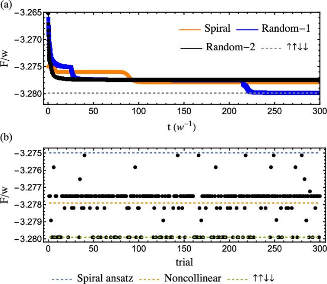
Figure 8. (a) Time evolution with three different initial conditions. The orange curve is for the optimal spiral, with an initial free energy Fs/w = −3.2750, relaxing to Feq/w = −3.2779. The other two curves have random initial states. The dashed line is the free energy F/w = −3.2799 of the ↑ ↑ ↓ ↓ configuration. (b) Asymptotic values Fi, obtained from 300 initial states. The top and middle dashed lines indicate Fs and Feq. The bottom dashed line is ${F}_{{\rm{\min }}}$, coinciding with the free energy of ↑ ↑ ↓ ↓ . In both panels, we used J/w = 1, μ/w =1.41, and L = 100. |
In figure 8(b), the value of ${F}_{\min }$ is indeed the energy of the ↑ ↑ ↓ ↓ state.
It is also interesting to consider parameters where the ground state is a noncollinear configuration. As shown in figure 9, which represents a refinement of figure 4(a) in the interval L = 300 –354, the free energy ${F}_{\min }$ obtained from random initial configurations (blue curve) is generally lower than Feq, which assumes the optimal spiral as initial state. Furthermore, ${F}_{\min }$ shows much weaker finite-size effects, compared to the oscillatory dependence of Feq. Despite these advantages, however, the gain in energy of these improved noncollinear states is small, since the difference ${F}_{{\rm{eq}}}-{F}_{\min }$ is always much smaller than Fs − Feq. Furthermore, ${F}_{{\rm{eq}}}-{F}_{\min }$ tends to decrease with system size. The spin configurations corresponding to Feq and ${F}_{{\rm{\min }}}$ are always qualitatively similar, and, in fact, the two states and energies are nearly identical at periodic values of L. Therefore, figure 9 indicates that the method employed in the main text of relying on Feq is both valid and significantly more computationally efficient, compared to using random initial configurations.

Figure 9. Finite-size scaling of the free energy, for the same parameters as in figure 4(a). Here we also include ${F}_{{\rm{\min }}}$, computed using 100 random initial conditions for each value of L. |