


1. Introduction
Networks of nonlinear coupled oscillators offer a powerful framework for understanding and capturing diverse emergent phenomena across various fields of science and technology. This research field has generated growing interest in the theoretical challenges arising at the interface of statistical mechanics and nonlinear dynamics [1–3].
The main challenge in current research lies in analyzing coupled systems with a high number of independent parameters, which have been shown to exhibit a wide range of intriguing collective phenomena and structural patterns. Theoretical studies have primarily concentrated on phase-only models, often neglecting amplitude effects under the assumption of weak coupling [4, 5].
Among coupled phase oscillators, one of the most prominent collective behaviors is the onset of synchronization. Specifically, synchronization describes a collective behavior where phase oscillators progressively align their motion through dissipative interactions, ultimately reaching a state of unison over time [6–10].
However, when the system involves interacting oscillators with strong coupling, amplitude effects become important, extending beyond the phase-only models. In this regard, amplitude variations cannot be ignored, leading to a variety of intriguing cooperative phenomena, as reported in many studies [11–22].
One particularly notable dynamic feature is oscillation quenching, a self-organized collective phenomenon that arises from the stabilization of an unstable equilibrium state [23]. In particular, this phenomenon is crucial for understanding and controlling associated oscillatory dynamics across various physical, chemical, biological and engineered systems [11, 24].
Previous studies of oscillation quenching have typically focused on systems where there is no correlation between the natural frequencies and oscillators’ amplitudes. However, recent investigations have shown that the presence of such a correlation, encoded by the shear diversity (nonisochronicity), can significantly shape the quenching dynamics of the oscillator systems [25–32]. For example, [30–32] suggested that shear diversity can significantly modify the critical point for synchronization onset within the phase reduction framework (weak coupling limit). However, to the best of our knowledge, no systematic study has been conducted to investigate the effects of shear diversity on oscillation quenching when both amplitude and phase responses are considered simultaneously.
In this study, we examine the quenching dynamics within a globally coupled oscillator network, considering both phase and amplitude responses. Specifically, we demonstrate that shear diversity has a critical influence on determining the onset of quenching dynamics. Beyond the phase-only model, we present a detailed stability analysis in terms of the limit-cycle kinetic theory with a continuous limit, which enables us to analytically locate the critical threshold characterizing the disappearance of oscillation quenching. Notably, we show that the interaction between the heterogeneous natural frequencies and shear diversity has a decisive impact on determining the characteristic equations and the eigenspectrum structure of the linearized system. Thus, our study offers valuable insights into the emergent mechanism of oscillation quenching in systems with inherent shear diversity, which can inform the design and control of oscillatory dynamics in complex systems.
The analytical framework is systematically developed as follows. In section 2 , we formulate the nonlinear dynamical system of coupled limit-cycle oscillators incorporating shear diversity. Section 3 includes a linear stability analysis of the incoherent state within the thermodynamic limit (N → ∞), establishing the critical point through spectral decomposition of the continuum operator. In section 4 , we investigate the effect of shear diversity on the critical coupling for various distributions. Finally, section 5 concludes the study.
2. Dynamical model with shear diversity
We begin by considering a dynamical model characterized by a system of limit-cycle oscillators with global coupling and disorder, which is
$\begin{eqnarray}\dot{{z}_{j}}=\left[1+{\rm{i}}\left({\omega }_{j}+{q}_{j}\right)-\left(1+{\rm{i}}{q}_{j}\right){\left|{z}_{j}\right|}^{2}\right]{z}_{j}+\frac{K}{N}\displaystyle \sum _{k=1}^{N}({z}_{k}-{z}_{j}).\end{eqnarray}$
Here, j = 1, 2, …, N represents the index of oscillators. The complex variable zj(t) = xj(t) + iyj(t) is the state of the jth oscillator at time t, with the overdot indicating the time derivative. ωj denotes the natural frequency of the jth oscillator. N ≫ 1 represents the system size and K > 0 characterizes the overall coupling strength between oscillators.Remarkably, qj accounts for the shear (or nonisochronicity), quantifying the dependence of the frequency and amplitude of the jth oscillator introduced in [30]. Typically, the natural frequencies and shears of equation (1 ) are distributed according to the densities g(ω) and h(q), respectively. Here and in the following, we assume that $\left\{{\omega }_{j}\right\}$ and $\left\{{q}_{j}\right\}$ are independent random variables, i.e. the joint probability density of ω and q can be expressed as p(ω, q) = g(ω)h(q). Furthermore, we assume that g(ω) and h(q) are unimodal and symmetric distributions; namely, g(ω) and h(q) are even functions and are non-increasing in the intervals ω > 0, q > 0, respectively.
The vast majority of works concerning equation (1 ) made the assumption that the heterogeneity solely originates from the intrinsic frequencies, i.e. qj ≡ 0. However, as reported in [30–32], the shear diversity, serving as a form of external fluctuation, must be considered to capture the underlying inhomogeneity of the oscillatory medium.
The coupling strategy presented in equation (1 ) extends the Stuart–Landau model, which provides the canonical description of interacting systems in the vicinity of the supercritical transition to oscillatory behavior. When there is no coupling (K = 0), the oscillators evolve independently, exhibiting limit-cycle motion with a unit radius following their respective natural frequencies and shears, i.e., ${z}_{j}(t)\sim {{\rm{e}}}^{{\rm{i}}({\omega }_{j}+{q}_{j})t}$. Upon introducing coupling, the cessation of oscillation occurs, resulting in the system reaching a stable state at equilibrium positions.
In [30–32], the authors attempted to explore the impact of shear diversity on oscillator quenching dynamics. In particular, they identified that shear diversity profoundly shapes the critical point for the emergence of collective synchronization. However, all previous investigations were limited to models based solely on phase dynamics, neglecting the impact of amplitude on the oscillators, and assumed weak coupling. In this work, we aim to advance and improve the stability analysis by retaining both the phase and amplitude responses, thereby offering a comprehensive approach for identifying the critical conditions that lead to the instability of the incoherent state in the presence of shear diversity.
3. Linear stability analysis
In this section, we focus on the stability of the incoherent state, where each oscillator moves independently along a circular trajectory determined by its natural frequency and shear, with varying radii. As highlighted previously, the incoherent state refers to a special form of quenching dynamics that essentially differs from other quenching states, such as amplitude death and oscillation death [33]. The stability of the incoherent state is characterized at the macroscopic scale, rather than being evident in the individual dynamics of the oscillators. Put differently, the incoherent state is defined by a zero macroscopic variable (mean-field), whereas the microscopic dynamics can exhibit rapid temporal fluctuations. To investigate the impact of shear diversity on the threshold for incoherent state instability, we undertake a comprehensive linear stability analysis that extends beyond the phase reduction framework outlined in [30–32].
To continue, it is useful to define an order parameter expressed as follows 1 ) can be reformulated into a mean-field approximation, which leads to 3 ) can be rewritten as two corresponding sets of differential equations
$\begin{eqnarray}Z(t)=R(t){{\rm{e}}}^{{\rm{i}}{\rm{\Theta }}(t)}=\frac{1}{N}\displaystyle \sum _{k=1}^{N}{z}_{k}(t),\end{eqnarray}$
where the complex quantity Z(t) represents the center of mass of the configuration $\left\{{z}_{k}\right\}$ on the two-dimensional complex space, with R(t) and Θ(t) corresponding to its modulus and phase angle, respectively. Thus, the evolution equation in equation ( $\begin{eqnarray}\dot{{z}_{j}}=\left[1-K+{\rm{i}}\left({\omega }_{j}+{q}_{j}\right)-\left(1+{\rm{i}}{q}_{j}\right){\left|{z}_{j}\right|}^{2}\right]{z}_{j}+KZ.\end{eqnarray}$
In the polar coordinates, ${z}_{j}(t)={r}_{j}(t){{\rm{e}}}^{{\rm{i}}{\theta }_{j}(t)}$, the mean-field equation in equation ( $\begin{eqnarray}\dot{{r}_{j}}=\left(1-K-{r}_{j}^{2}\right){r}_{j}+K{\rm{Re}}\left(Z{{\rm{e}}}^{-{\rm{i}}{\theta }_{j}}\right),\end{eqnarray}$
$\begin{eqnarray}\dot{{\theta }_{j}}={\omega }_{j}+{q}_{j}-{q}_{j}{r}_{j}^{2}+\frac{K}{{r}_{j}}{\rm{Im}}\left(Z{{\rm{e}}}^{-{\rm{i}}{\theta }_{j}}\right).\end{eqnarray}$
To perform the stability analysis of the incoherent state, we now express differential equations (4 ) and (5 ) in the limit of large N. Alternatively, equation (1 ) can be represented by a distribution function $\rho \left(r,\theta ,\omega ,q,t\right)$, in such a way that ρdrdθdωdq corresponds to the proportion of oscillators within the ranges $\left(r,r+{\rm{d}}r\right)\cup \left(\theta ,\theta +{\rm{d}}\theta \right)\cup \left(\omega ,\omega +{\rm{d}}\omega \right)\cup \left(q,q+{\rm{d}}q\right)$ at the specified time t. Additionally, the distribution function must comply with the normalization condition
$\begin{eqnarray}\begin{array}{l}{\displaystyle \int }_{0}^{\infty }{\rm{d}}r{\displaystyle \int }_{0}^{2\pi }{\rm{d}}\theta {\displaystyle \int }_{-\infty }^{\infty }{\rm{d}}\omega {\displaystyle \int }_{-\infty }^{\infty }{\rm{d}}q\rho \left(r,\theta ,\omega ,q,t\right)\\ \,\times g(\omega )h(q)=1.\end{array}\end{eqnarray}$
Similarly, in the continuous limit, the order parameter is given by $\begin{eqnarray}\begin{array}{rcl}Z(t) & = & {\displaystyle \int }_{0}^{\infty }{\rm{d}}r{\displaystyle \int }_{0}^{2\pi }{\rm{d}}\theta {\displaystyle \int }_{-\infty }^{\infty }{\rm{d}}\omega {\displaystyle \int }_{-\infty }^{\infty }{\rm{d}}q\\ & & \times r{{\rm{e}}}^{{\rm{i}}\theta }\rho \left(r,\theta ,\omega ,q,t\right)g(\omega )h(q).\end{array}\end{eqnarray}$
For simplicity, we have dropped the index of each oscillator in the continuous limit.
As for the incoherent state, all the oscillators move at their respective natural frequencies and shears on the circle ${r}_{j}=\sqrt{1-K}$, i.e. the introduction of the coupling between the oscillators reduces the amplitude of the individual limit cycles from 1 to $\sqrt{1-K}$. As a result, the distribution of the incoherent state is expressed as 1 ), the probability distribution satisfies the continuity equation of the form
$\begin{eqnarray}{\rho }_{0}\left(r,\theta ,\omega ,q\right)=\frac{\delta \left(r-\sqrt{1-K}\right)}{2\pi },\end{eqnarray}$
in which δ( · ) indicates the Dirac delta function. Rather than equation ( $\begin{eqnarray}\frac{\partial \rho }{\partial t}+{\boldsymbol{\nabla }}\cdot \left(\rho {\boldsymbol{v}}\right)=0,\end{eqnarray}$
where ∇ represents the vector field divergence and the flow field is given by ${\boldsymbol{v}}=(\dot{r},r\dot{\theta })$. Consequently, the continuity equation in terms of polar representation leads to $\begin{eqnarray}\frac{\partial \rho }{\partial t}+\frac{\partial }{\partial r}(\rho \dot{r})+\frac{\partial }{\partial \theta }(\rho \dot{\theta })=0,\end{eqnarray}$
with $\begin{eqnarray}\dot{r}=\left(1-K-{r}^{2}\right)r+\frac{K}{2}\left(Z{{\rm{e}}}^{-{\rm{i}}\theta }+\bar{Z}{{\rm{e}}}^{{\rm{i}}\theta }\right),\end{eqnarray}$
and $\begin{eqnarray}\dot{\theta }=\omega +q-q{r}^{2}+\frac{K}{r}\frac{1}{2{\rm{i}}}\left(Z{{\rm{e}}}^{-{\rm{i}}\theta }-\bar{Z}{{\rm{e}}}^{{\rm{i}}\theta }\right).\end{eqnarray}$
From this point onward, “$\bar{\cdot }$” will denote the complex conjugate. It should be emphasized that the vector field divergence is expressed in polar form $\left({\boldsymbol{\nabla }}=\frac{\partial }{\partial r}+\frac{1}{r}\frac{\partial }{\partial \theta }\right)$.Next, we perform a linearization of equation (10 ) around the fixed point given in equation (8 ). To achieve this, we apply a small perturbation to equation (8 ), that is
$\begin{eqnarray}\rho (r,\theta ,\omega ,q,t)=\frac{\delta (r-\sqrt{1-K})}{2\pi }+\delta \rho (r,\theta ,\omega ,q,t).\end{eqnarray}$
Owing to the normalization condition, the perturbated function satisfies $\begin{eqnarray}{\int }_{0}^{\infty }{\rm{d}}r{\int }_{0}^{2\pi }{\rm{d}}\theta {\int }_{-\infty }^{\infty }{\rm{d}}\omega {\int }_{-\infty }^{\infty }{\rm{d}}q\delta \rho \left(r,\theta ,\omega ,q,t\right)=0.\end{eqnarray}$
As a result, the corresponding order parameter under the perturbation takes the form of $\begin{eqnarray}\begin{array}{rcl}\delta Z(t) & = & {\displaystyle \int }_{0}^{\infty }{\rm{d}}r{\displaystyle \int }_{0}^{2\pi }{\rm{d}}\theta {\displaystyle \int }_{-\infty }^{\infty }{\rm{d}}\omega {\displaystyle \int }_{-\infty }^{\infty }{\rm{d}}q\\ & & \times r{{\rm{e}}}^{{\rm{i}}\theta }\delta \rho \left(r,\theta ,\omega ,q,t\right)g(\omega )h(q).\end{array}\end{eqnarray}$
Given that the distribution is 2π-periodic in θ, it follows that its Fourier series can be expressed as 14 ) and that $\delta {\rho }_{n}=\delta {\bar{\rho }}_{-n}$ due to the real-valued nature of δρ. As can be observed from equation (15 ), the order parameter is exclusively determined by δρ−1, implying that higher-order Fourier coefficients do not contribute to the subsequent analysis. Thus, it is adequate to focus on the first Fourier subspace for further analysis.
$\begin{eqnarray}\delta \rho \left(r,\theta ,\omega ,q,t\right)=\displaystyle \sum _{n=-\infty }^{\infty }\delta {\rho }_{n}\left(r,\omega ,q,t\right){{\rm{e}}}^{{\rm{i}}n\theta },\end{eqnarray}$
in which $\delta {\rho }_{n}\left(r,\omega ,q,t\right)$ represents the nth Fourier coefficient. It is worth noting that δρ0 = 0 as a result of the normalization condition in equation (In accordance with the linear stability analysis approach, we assume the forms δρ±1(t) = δρ±1eλt and δZ(t) = δZeλt. By substituting these expressions into equation (10 ) and matching the coefficients of the terms e±iθ, we derive the linear evolution equation for the first-order Fourier mode, which is given by
$\begin{eqnarray}\begin{array}{l}\left[\lambda -{\rm{i}}\left(\omega +q-q{r}^{2}\right)\right]\delta {\rho }_{-1}+\frac{\partial }{\partial r}\left[\left(1-K-{r}^{2}\right)r\delta {\rho }_{-1}\right]\\ \quad =\frac{K\delta Z}{4\pi }\left[\frac{\delta (r-\sqrt{1-K})}{r}-{\delta }^{{}^{{\prime} }}(r-\sqrt{1-K})\right],\end{array}\end{eqnarray}$
where ${\delta }^{{\prime} }(\cdot )$ represents the differential of the Dirac delta function with respect to its argument. Notably, the specific structure of the right-hand term of equation (17 ) allows us to adopt the following assumption for δρ−1, which leads to
$\begin{eqnarray}\begin{array}{rcl}\delta {\rho }_{-1} & = & \frac{K\delta Z}{4\pi }[{C}_{1}(\omega ,q)\delta (r-\sqrt{1-K})\\ & & +{C}_{2}(\omega ,q){\delta }^{{}^{{\prime} }}(r-\sqrt{1-K})],\end{array}\end{eqnarray}$
where C1,2(ω, q) are the constants that need to be determined.By inserting equation (18 ) to equation (17 ) and applying the properties for the Dirac delta function, i.e.18 ) and equation (23 )∼equation (24 ) with equation (15 ), we derive the order parameter under the perturbation, resulting in
$\begin{eqnarray}f(x)\delta (x-a)=f(a)\delta (x-a)\end{eqnarray}$
and $\begin{eqnarray}f(x){\delta }^{{\prime} }(x-a)=f(a){\delta }^{{\prime} }(x-a)-{f}^{{\prime} }(a)\delta (x-a).\end{eqnarray}$
This leads to a closed-form equation for the coefficients C1,2, given by $\begin{eqnarray}\left[\lambda -{\rm{i}}(\omega +qK)\right]{C}_{1}-2\sqrt{1-K}q{\rm{i}}{C}_{2}=\displaystyle \frac{1}{\sqrt{1-K}}\end{eqnarray}$
and $\begin{eqnarray}\left[\lambda -{\rm{i}}(\omega +qK)\right]{C}_{2}+2(1-K){C}_{2}=-1.\end{eqnarray}$
Straightforward computations yield $\begin{eqnarray}\begin{array}{rcl}{C}_{1} & = & \displaystyle \frac{1}{\sqrt{1-K}\left[\lambda -{\rm{i}}(\omega +qK)\right]}\\ & & -\displaystyle \frac{2\sqrt{1-K}q{\rm{i}}}{\left[\lambda +2(1-K)-{\rm{i}}(\omega +qK)\right]\left[\lambda -{\rm{i}}(\omega +qK)\right]}\end{array}\end{eqnarray}$
and $\begin{eqnarray}{C}_{2}=-\frac{1}{\lambda +2(1-K)-{\rm{i}}(\omega +qK)}.\end{eqnarray}$
By combining equation ( $\begin{eqnarray}\begin{array}{rcl}\delta Z & = & {\displaystyle \int }_{0}^{\infty }{\rm{d}}r{\displaystyle \int }_{0}^{2\pi }{\rm{d}}\theta {\displaystyle \int }_{-\infty }^{\infty }g(\omega ){\rm{d}}\omega {\displaystyle \int }_{-\infty }^{\infty }h(q){\rm{d}}qr{{\rm{e}}}^{{\rm{i}}\theta }\delta {\rho }_{-1}{{\rm{e}}}^{-{\rm{i}}\theta }\\ & = & 2\pi {\displaystyle \int }_{0}^{\infty }{\rm{d}}r{\displaystyle \int }_{-\infty }^{\infty }g(\omega ){\rm{d}}\omega {\displaystyle \int }_{-\infty }^{\infty }h(q){\rm{d}}qr\delta {\rho }_{-1}\\ & = & \frac{K\delta Z}{2}{\displaystyle \int }_{0}^{\infty }{\rm{d}}r{\displaystyle \int }_{-\infty }^{\infty }g(\omega ){\rm{d}}\omega {\displaystyle \int }_{-\infty }^{\infty }h(q){\rm{d}}q\\ & & \times r\left[{C}_{1}\delta (r-\sqrt{1-K})+{C}_{2}{\delta }^{{\prime} }(r-\sqrt{1-K})\right]\\ & = & \frac{K\delta Z}{2}{\displaystyle \int }_{-\infty }^{\infty }g(\omega ){\rm{d}}\omega {\displaystyle \int }_{-\infty }^{\infty }h(q){\rm{d}}q\\ & & \times \left[\frac{1}{\lambda -{\rm{i}}(\omega +qK)}+\frac{1}{\lambda +2(1-K)-{\rm{i}}(\omega +qK)}\right.\\ & & \left.-\frac{2(1-K)q{\rm{i}}}{\left[\lambda +2(1-K)-{\rm{i}}(\omega +qK)\right]\left[\lambda -{\rm{i}}(\omega +qK)\right]}\right].\end{array}\end{eqnarray}$
Ultimately, we obtain the self-consistent equation that governs the eigenvalues of the linearized system around the incoherent state, which gives
$\begin{eqnarray}\frac{2}{K}={I}_{1}+{I}_{2}-{I}_{3},\end{eqnarray}$
with $\begin{eqnarray}{I}_{1}={\int }_{-\infty }^{\infty }{\int }_{-\infty }^{\infty }\frac{1}{\lambda -{\rm{i}}(\omega +qK)}g(\omega )h(q){\rm{d}}\omega {\rm{d}}q,\end{eqnarray}$
$\begin{eqnarray}{I}_{2}={\int }_{-\infty }^{\infty }{\int }_{-\infty }^{\infty }\frac{1}{\lambda +2(1-K)-{\rm{i}}(\omega +qK)}g(\omega )h(q){\rm{d}}\omega {\rm{d}}q,\end{eqnarray}$
$\begin{eqnarray}\begin{array}{rcl}{I}_{3} & = & {\displaystyle \int }_{-\infty }^{\infty }{\displaystyle \int }_{-\infty }^{\infty }\frac{2(1-K)q{\rm{i}}}{\lambda +2(1-K)-{\rm{i}}(\omega +qK)}\\ & & \times \frac{1}{\lambda -{\rm{i}}(\omega +qK)}g(\omega )h(q){\rm{d}}\omega {\rm{d}}q.\end{array}\end{eqnarray}$
It is evident that the stability of the incoherent state is entirely determined by the real parts of the eigenvalues λ. In particular, the linear stability condition mandates that all eigenvalues lie in the left half of the complex plane.The incoherent state becomes linearly unstable when the eigenvalues move across the imaginary axis. In particular, due to the symmetrical properties of g(ω) and h(q), λ is shown to be real. The critical point Kc, indicating the onset of instability in the incoherent state, is located by applying the critical condition λ → 0+. This is because, in the case of continuous parameter variation, the stability of the system is generally determined by the sign of the eigenvalues, whereas oscillation quenching is typically triggered when λ crosses a critical value. Here, instability occurs when λ changes from negative to positive; therefore, the first instability point must correspond to λ → 0+, which is
$\begin{eqnarray}\begin{array}{rcl}\frac{1}{{K}_{c}} & = & \frac{\pi }{2}{\displaystyle \int }_{-\infty }^{\infty }g(-q{K}_{c})h(q){\rm{d}}q+{\displaystyle \int }_{-\infty }^{\infty }{\displaystyle \int }_{-\infty }^{\infty }\frac{1-{K}_{c}}{\omega +q{K}_{c}}\\ & & \times \frac{\omega +q(2+{K}_{c})}{{(\omega +q{K}_{c})}^{2}+4{(1-{K}_{c})}^{2}}g(\omega )h(q){\rm{d}}\omega {\rm{d}}q.\end{array}\end{eqnarray}$
Considering the special forms g(ω) and h(q), the critical coupling strength Kc may be evaluated analytically. For instance, if h(q) = δ(q) (vanishing shear diversity), we have that $\begin{eqnarray}\frac{1}{{K}_{c}}=\frac{\pi }{2}g(0)+{\int }_{-\infty }^{\infty }\frac{1-{K}_{c}}{{\omega }^{2}+4{(1-{K}_{c})}^{2}}g(\omega ){\rm{d}}\omega .\end{eqnarray}$
The implicit dependence of Kc on frequency distribution (intrinsic diversity) recovers the results of the classical Stuart–Landau model [14].4. Mathematical consequences of shear diversity
In order to appreciate the impacts of shear diversity on the critical threshold, we next showcase several scenarios by specifying on some distributions of g(ω) and h(q).
We begin by examining the scenario of identical oscillators, i.e. g(ω) = δ(ω). In this scenario, the closed form deciding the critical coupling strength Kc is expressed as
$\begin{eqnarray}\begin{array}{rcl}\frac{1}{{K}_{c}} & = & \frac{\pi h(0)}{2{K}_{c}}+\frac{(1-{K}_{c})(2+{K}_{c})}{{K}_{c}}\\ & & \times {\displaystyle \int }_{-\infty }^{\infty }\frac{1}{{(q{K}_{c})}^{2}+4{(1-{K}_{c})}^{2}}h(q){\rm{d}}q.\end{array}\end{eqnarray}$
To proceed, we exemplify three typical distributions of shear to elucidate the critical coupling. For the scenario involving a uniform distribution, i.e.34 ) should be solved numerically to obtain the relation between Kc and γ (figure 1).
$\begin{eqnarray}h(q)=\left\{\begin{array}{cc}\displaystyle \frac{1}{2\gamma }, & q\in (-\gamma ,\gamma )\\ 0, & \mathrm{otherwise};\end{array}\right.\end{eqnarray}$
here, γ is interpreted as a measure describing the shear diversity. Therefore, the critical coupling strength is given by the following transcendental equation, which yields $\begin{eqnarray}\frac{1}{{K}_{c}}=\frac{\pi }{4{K}_{c}\gamma }+\frac{(1-{K}_{c})(2+{K}_{c})}{{K}_{c}}\frac{\arctan \left(\frac{{K}_{c}\gamma }{2-2{K}_{c}}\right)}{2{K}_{c}\gamma -2{K}_{c}^{2}\gamma }.\end{eqnarray}$
Correspondingly, equation (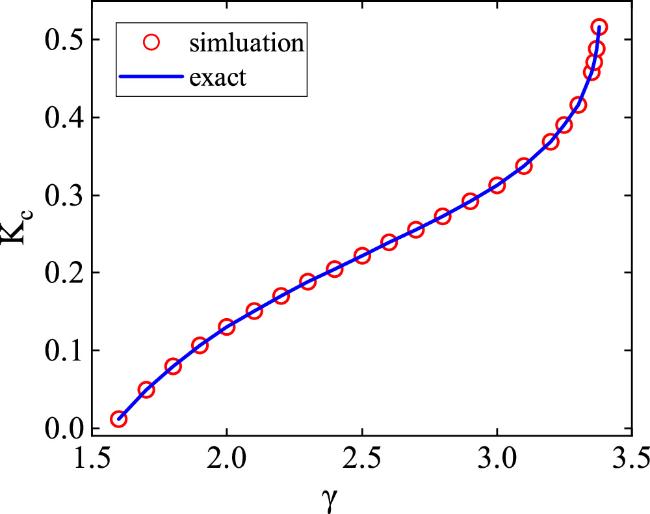
Figure 1. The critical coupling strength Kc as a function of the uniform distribution parameter γ is shown. The blue solid line corresponds the theoretical prediction by equation ( |
For the scenario of a parabolic distribution, i.e.
$\begin{eqnarray}h(q)=\left\{\begin{array}{ll}\frac{3}{4}\frac{{\gamma }^{2}-{q}^{2}}{{\gamma }^{3}}, & q\in (-\gamma ,\gamma )\\ 0, & {\rm{otherwise}}\end{array}\right.\end{eqnarray}$
and γ reflects the shear diversity. Consequently, the coupling strength Kc is determined by the following complicated transcendental equation, which reads $\begin{eqnarray}\begin{array}{rcl}\frac{1}{{K}_{c}} & = & \frac{3\pi }{8{K}_{c}\gamma }+\frac{(1-{K}_{c})(2+{K}_{c})}{{K}_{c}}\left[-\frac{3\left(({K}_{c}-1)\pi +{K}_{c}\gamma \right)}{2{K}_{c}^{3}{\gamma }^{3}}\right.\\ & & -\left.\frac{3({K}_{c}-1)\arctan \left(\frac{2{K}_{c}-2}{{K}_{c}\gamma }\right)}{{K}_{c}^{3}{\gamma }^{3}}+\frac{3\arctan \left(\frac{{K}_{c}\gamma }{2-2{K}_{c}}\right)}{4{K}_{c}\gamma -4{K}_{c}^{2}\gamma }\right].\end{array}\end{eqnarray}$
Also, the general relation between Kc and γ is illustrated in figure 2.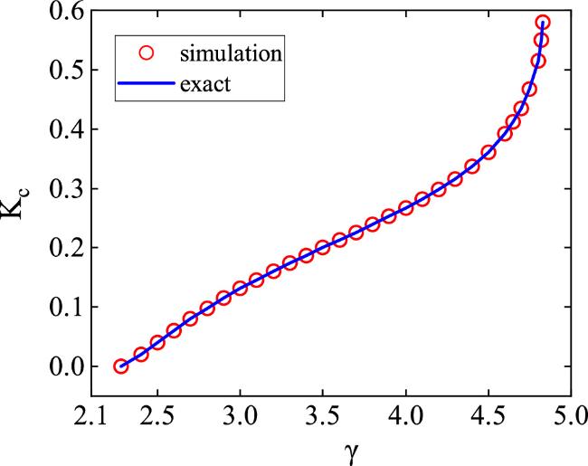
Figure 2. The critical coupling strength Kc as a function of the parabolic distribution parameter γ is shown. The blue solid line corresponds the theoretical prediction by equation ( |
We now turn to consider the case in which the shear distribution has an infinite support. Specifically, h(q) is selected as a Lorentzian distribution expressed as
$\begin{eqnarray}h(q)=\frac{\gamma /\pi }{{q}^{2}+{\gamma }^{2}},q\in \left(-\infty ,\infty \right).\end{eqnarray}$
Notably, the critical coupling strength Kc can be represented by a straightforward expression, resulting in $\begin{eqnarray}{K}_{c}=\frac{1-\gamma }{1-3\gamma +{\gamma }^{2}}.\end{eqnarray}$
The associated results are depicted in figure 3.
Figure 3. The critical coupling strength Kc as a function of the Lorentzian distribution parameter γ is shown. The blue solid line corresponds the theoretical prediction by equation ( |
In contrast to case of the identical oscillators, we next consider the nonidentical scenario with distributed frequencies to further examine the influences of both types of diversity on the critical threshold. To this end, we choose g(ω) and h(q) to be the Lorentzian form with different widths, i.e.39 ) into equation (30 ) as shown in figure 4.
$\begin{eqnarray}g(\omega )=\frac{\delta /\pi }{{\omega }^{2}+{\delta }^{2}},h(q)=\frac{\gamma /\pi }{{q}^{2}+{\gamma }^{2}},\omega ,q\in \left(-\infty ,\infty \right).\end{eqnarray}$
Unlike the situations of the identical oscillators discussed above, we point out that it is difficult to obtain an explicit formula of the closed form concerning the critical coupling. Nevertheless, the results can be solved numerically by inserting equation (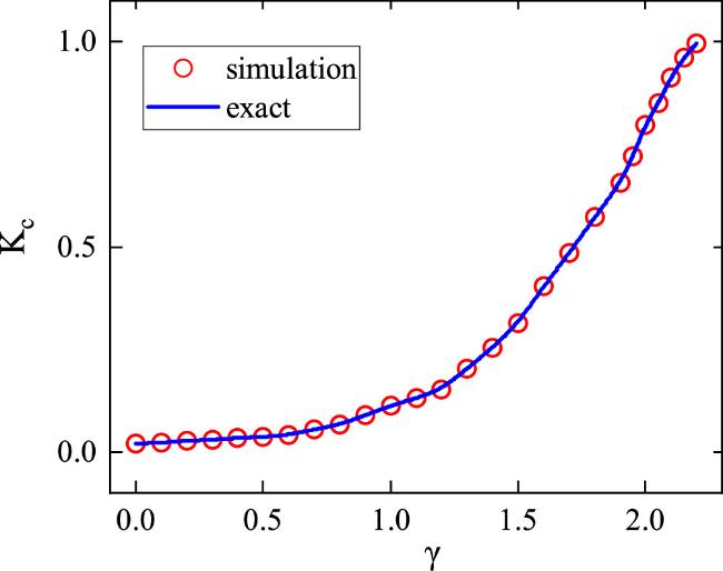
Figure 4. The critical coupling strength Kc as a function of the Lorentzian distribution parameters γ and δ = 0.01 is shown. The blue solid line corresponds the theoretical prediction through numerical integration equation ( |
Taken together, the critical coupling strength Kc as functions of shear diversity parameters are illustrated in figures 1–4. It is shown that the critical coupling strength Kc exhibits monotonically increasing behaviors with the diversity parameters for both identical and nonidentical oscillator populations, and the analytical predictions (lines) coincide well with the numerical simulations (circles). These plots demonstrate that the increment of shear diversity tend to inhibit the instability of the incoherent state, thereby making it more difficult for the system to reach the coherent states.
Previous research has demonstrated that shear diversity plays a crucial role in shaping the onset of synchronization within the context of phase reduction models. Interestingly, it was found that increasing shear diversity delays the critical threshold for phase synchronization onset, with this threshold diverging at a specific value of the shear diversity parameter. When both the amplitude and phase effects are considered simultaneously, we remark that the tendency of stabilizing the incoherent state inducing by the shear diversity is maintained. In other words, the shear diversity is prone to postpone the occurrence of the rhythmic states. However, in contrast to the phase-only models, we highlight that the critical coupling strength Kc in the amplitude-phase scenario remains finite. This is due to the fact that the interplay between the phases and amplitudes of the oscillators demands that the existent condition for the incoherent state is $K\in \left[0,1\right]$. Nevertheless, we emphasize that the critical coupling exists only in a certain range of γ (shear diversity) for the identical oscillators, whereas it exists in the whole range of γ for the nonidentical oscillator populations given that Kc < 1. Mathematically, the particular dependence of the critical coupling Kc on the shear diversity parameter γ is governed by the transcendental properties of the characteristic equations. Beyond the existent region of Kc, the system gives rise to fascinating rhythmic dynamics that will be reported elsewhere.
5. Conclusion
In summary, we explored the quenching dynamics induced by the shear diversity in a globally coupled oscillator system by taking into account both phase and amplitude responses. As reported in previous studies, the distributed shear in the phase-only models (e.g. Kuramoto-like models) hinders the emergence of phase synchronization and even makes it impossible at a certain range of the shear diversity [30]. In this work, we demonstrated that the amplitude and phase responses combine together to affect the onset of collective dynamics under the influence of shear diversity. Specifically, we found that the added shear diversity tends to inhibit the occurrence of coherent behavior, even when amplitude effects are suppressed. Nevertheless, we revealed that the critical coupling Kc, featuring the instability of the incoherent state (macroscopic quenching dynamics), exhibits a monotonically increasing function with respect to the parameter of shear diversity that can never diverge owing to the restricted region of the incoherent state.
Theoretically, we developed a general framework for systemically performing linear stability analysis of incoherent states that goes beyond phase-reduction models. We analytically derived the eigenvalue spectrum of the linearized system, explicitly accounting for the nonlinear amplitude-phase coupling inherent in limit-cycle ensembles. Consequently, the critical coupling strengths were formulated in terms of several transcendental equations (equations (34 ) and (36 )). This study establishes a robust theoretical framework that advances the investigation of diversity-mediated amplitude suppression phenomena in nonlinear dynamic systems, while simultaneously developing a unified analytical paradigm for characterizing synchronization stability in networks of coupled limit-cycle oscillators.