


1. Introduction
In many cities, urban rail transit has become one of the most popular modes of transportation for passengers [1]. The operation of urban rail transit has increased the supply of public transport and shared the travel demand of passengers [2]. The development of urban rail transit has made great contributions to alleviating the pressure of urban transport and promoting green transport [3]. China's urban rail transit has been gradually improved after decades of development, and many cities have stepped into the situation of networked operation [4]. According to the official news from China Association of Metros, a total of 59 cities in Mainland China have introduced urban rail transit, reaching 11232.65 kilometers in operating mileage. Beijing is the capital of China, with a relatively robust urban rail transit interchange topology (URTIT) network.
Meanwhile, the technology of operating urban rail transit is also constantly evolving [5]. At present, the new technologies applied in China's urban rail transit operating lines mainly include self−driving technology and magnetic levitation technology. For example, Beijing Subway Capital Airport Express is a self−driving train, and Beijing Subway Line S1 is a maglev line that utilizes magnetic levitation technology.
In general, the relationship between the application of new technologies and passenger travel behavior is that the former affects the latter. On the one hand, the application of new technologies changes the passenger mode so that passengers who originally chose other modes newly switch to urban rail transit. On the other hand, the application of new technologies changes passenger route choice, generally reflected in the passenger volume of neighboring lines. When a new technology is applied to a line of urban rail transit, it will have an impact on other lines and even the entire urban rail transit network. However, few studies focus on this issue. In fact, it would be interesting to explore the influence propagation mechanism, including the influence range [6], the influence propagation paths [7], and the influence intensity [8].
In this paper, we analyze the impact of applying new technologies on passenger travel behavior of urban rail transit, considering lines of urban rail transit as nodes of the network. Gravity models [9] can be used to portray the intensity of influence, but most models are not path−based. Therefore, we put forward an improved path−based gravity (IPG) model. The contributions of this paper are as follows.
(1).From a holistic perspective, this paper constructs the URTIT network by taking urban rail transit lines as nodes and interchange relationships as edges to portray the mutual relationships among lines.
(2).A unique influence propagation mechanism is considered. We define the influence radius to describe the influence range and propose the IPG model based on the influence propagation path to measure the influence intensity.
(3).We quantify the impact of applying new technologies on passenger travel behavior of urban rail transit and conduct sensitivity analysis to illustrate the effects of parameters and variables.
From a practical perspective, this paper explores the impact of the application of new technologies on passenger travel behavior in urban rail transit. Based on the work of this paper, it is possible to quantify the carbon emission reduction of applying new technologies in urban rail transit. Relevant research provides some reference for management in the process of formulating policies to meet the low-carbon goals.
The rest of this paper is organized as follows. Section 2 summarizes the existing literature; section 3 mainly introduces the methodologies proposed in this paper; section 4 presents the case study; section 5 describes the conclusions.
2. Literature review
The continuous improvement of social development level has promoted the process of urbanization, which has led to an increase in the number of urban residents and private cars, further leading to problems such as traffic congestion and air pollution [10]. In reality, traffic congestion exists in many cities, which has a negative impact on the daily lives of residents to varying degrees due to many factors such as overpopulation of the city, limited capacity of the transportation system, and the demand for similar travel time [11]. Prioritizing the development of public transport is an important way to alleviate these problems. Especially as an important component of public transport, urban rail transit has developed rapidly because of its advantages of high efficiency and environmental protection in recent years [12].
At present, scholars have done a lot of research work on passenger travel behavior of urban rail transit, containing many research directions, such as passenger characteristics and prediction [13, 14], and analysis of factors affecting passenger travel behavior [15]. The factors mainly consider time, price, weather, and so on. However, few scholars consider the impact of applying new technologies on the passenger travel behavior of urban rail transit.
As a matter of fact, with the development of technology, the train operation control system based on communication technology is continuously investigated. Some cities have already used a Communication Based Train Control (CBTC) system [16], which is the core of the current mobile occlusion technology in urban rail transit operations. According to the actual situation of the urban rail transit operation, automatic train operation (ATO) [17] is usually adopted at this stage, which can realize train operation automatic adjustment, speed control and regulation, common braking and precise stopping, automatic folding back, controlling doors, energy-saving operation, fault alarms, and data recording. In addition, magnetic levitation technology is also used in urban rail transit systems, having relatively low noise and vibration [18]. Maglev trains are a relatively new type of urban rail transit, which can realize the levitation of the train and the track using electrically generated magnetic levitation technology [19]. China has mastered the medium and low-speed maglev trains with independent intellectual property rights, such as the completed Beijing Subway Line S1. It adopts the principle of electromagnetic levitation, much safer and environmentally friendly. In this way, it is necessary to explore the impact of applying new technologies on passenger travel behavior of urban rail transit as technologies develop rapidly.
Urban rail transit is a typical complex system [20]. In fact, complex systems exist widely, which can be described by different complex networks [21]. The URTIT network can be abstracted as a complex network to study and solve the problems related to urban transportation. The complex network is composed of several nodes and edges, which can reflect the relationships among individuals in the system [22, 23]. The modeling methods of network topology mainly include Space−L, Space−P, and Space−C [24]. Among them, the Space−L and Space−P methods take the station as the network node, while the Space−C method takes the line as the network node, and establishes edge relationships between the two lines with transfer stations [25].
Many scholars have built the topological network of urban rail transit based on complex network methods and conducted a series of studies. Zhou et al [26] considered the basic statistical characteristics of complex network topology and constructed a P−center site selection model for emergency service stations of urban rail transit. Xu et al [27] took the urban rail transit system in Shanghai as an example to construct a network topology model, calculated the characteristics of the network structure, and analyzed the destruction resistance of a giant urban rail transit network with scale growth from a vulnerability perspective. Based on complex network theory, Wan et al [28] proposed a hybrid topology structure method to identify the critical nodes in the urban rail transit network and achieve high performance.
Furthermore, the problem of influence propagation based on complex networks has attracted the attention of researchers in recent years. Different scholars have differences in the setting of influence propagation mechanisms as they focus on different aspects. Generally speaking, the influence propagation mechanism mainly considers the influence propagation path, influence intensity, and influence range. The propagation path of the influence can be determined according to the propagation modes among nodes [29]. The influence propagation model [30] can analyze the interaction patterns between two nodes based on their influence. At present, the most widely used influence propagation models include the independent cascade (IC) model [31] and the linear threshold (LT) model [32]. The IC model is a probabilistic model, and the LT model is a value accumulation model [33]. Subsequently, scholars improved the basic model and put forward some improved versions.
Moreover, the gravity model is a widely used interaction model that can measure the magnitude of the influence between two different objects [34]. An important characteristic of the gravity model is that its basic form remains unchanged, and gravity models can be applied to different problems as long as the definitions of parameters and components are appropriately changed [35]. In order to improve some aspects of the model, scholars have improved the basic model. Currently, many beneficial research results have been achieved in economy [36], transportation [37], and other fields.
There are some gaps in current research. Topological network nodes of urban rail transit are often stations, rather than lines. The wholeness of lines is ignored. In addition, different influence propagation mechanisms have been investigated by scholars focusing on certain aspects. How to design a comprehensive and rational influence propagation mechanism is still an important matter. For example, we can describe the influence range with a kind of reliable index. Both distance and time factors can be considered when looking for the influence propagation paths. And few studies have considered path−based gravity models, which is a direction we can improve. Finally, few studies have focused on the impact of applying new technologies on the passenger travel behavior of urban rail transit, which will be explored.
3. Methodology
3.1. Problem and description
Urban rail transit has become an important way of public transport. The level of technology in various fields, including urban rail transit, keeps advancing to meet the needs of reality. Passenger travel behavior will be potentially affected by new technologies. When a new technology is adopted in a particular urban rail transit line, it will affect other lines and even the whole urban rail transit network. However, few studies have focused on scenarios regarding the application of new technologies in urban rail transit and the impact on passenger travel behavior. Therefore, this paper aims to explore the impact of applying new technologies on passenger travel behavior of urban rail transit.
The development of complex network theory provides an ingenious method for the study of URTIT networks. The topological network nodes of urban rail transit are generally stations, rather than lines. It reflects that the wholeness of lines is neglected. In addition, many studies have investigated influence propagation mechanisms that focus on certain aspects, which are relatively incomplete. Especially, few studies have considered path−based gravity models, while we propose the IPG model to measure the intensity of influence.
Space−C method is a network construction method based on the theory of complex networks. It is usually used to convert a transportation network into a topological network. This method abstracts the lines as nodes, and considers the relationships among the lines as connected edges. In general, if two lines can interchange at the same station, it can be simplified to two nodes with connected edges according to the Space−C method. In this paper, the Space−C method is used to construct the URTIT network. Based on the principle of wholeness, this paper takes the lines of urban rail transit as nodes, establishes edges for the interchange relationships, and considers the corresponding gray correlation coefficients [38] as the edge weights.
In order to analyze the impact of applying new technologies on the passenger travel behavior of urban rail transit, this paper considers a unique influence propagation mechanism, which is mainly divided into three aspects: influence range, influence propagation path, and influence intensity. The determination of the threshold value is one of the important elements of the influence propagation mechanism. The influence range is based on the influence radius, and the influence propagation paths are searched based on distance and time. This paper improves the gravity model to measure the intensity of influence based on the influence propagation paths.
The total flow of the model framework in this paper is shown in figure 1.
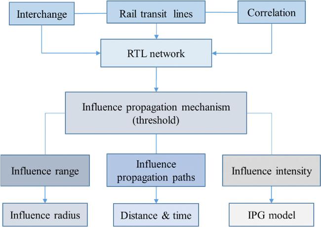
Figure 1. The total flow of the model framework. |
3.2. Construction of the URTIT network
In this paper, the URTIT network is proposed based on the networked method. In general, the complex network is composed of some nodes and edges. The nodes represent the elements, and the edges represent the relationships among the elements. Therefore, the URTIT network can be expressed as $G=(V,E)$, where $G$ represents the URTIT network; $V$ represents the collection of urban rail transit lines; and $E$ represents the set of interchange relationships among lines. In the following, the URTIT network will be specifically introduced.
3.2.1. Nodes
The URTIT network constructed in this paper considers lines of urban rail transit as nodes to explore the influence among different lines from a macroscopic perspective. In the network, there is a basic index about nodes called degree. The number of nodes connected to node $i$ is the degree of node $i$.
3.2.2. Edges
The edges of the network represent the relationships among nodes, which specifically refers to the interchange relationships among different lines of urban rail transit. A unique adjacency matrix [39] can be displayed based on interchange relationships for subsequent construction of the URTIT network. In general, we assume that there are $m$ nodes. The adjacency matrix can be expressed as:
$\begin{eqnarray}A=\left[\begin{array}{cccc}0 & {\delta }_{12} & \cdots & {\delta }_{1m}\\ {\delta }_{21} & 0 & \cdots & {\delta }_{2m}\\ \vdots & \vdots & \ddots & \vdots \\ {\delta }_{m1} & {\delta }_{m2} & \cdots & 0\end{array}\right],\end{eqnarray}$
where ${\delta }_{ij}$ is a 0−1 variable. If ${\delta }_{ij}=1$, it means that there is an interchange relationship. Otherwise, there is no interchange relationship.3.2.3. Edge weights
Based on the adjacency matrix, this paper takes the gray correlation coefficients among different nodes as the edge weights of the URTIT network. It is assumed that there are reference sequences and comparison sequences as follows:
$\begin{eqnarray}{X}_{0}=\{{x}_{0}(k)| k=1,2,\cdots ,n\},\,{X}_{i}=\{{x}_{i}(k)| i=1,2,\cdots ,m\}.\end{eqnarray}$
In equation (2 ), ${X}_{0}=\{{x}_{0}(k)| k=1,2,\cdots ,n\}$ represents the reference sequences, the data series that can reflect the behavior of the system; ${X}_{i}=\{{x}_{i}(k)| i=1,2,\cdots ,m\}$ represents the comparison sequences, the data series consisting of factors that influence the behavior of the system; $n$ is the year; and $m$ is the number of nodes. Equation (2 ) is a general setting for calculating the gray correlation coefficients as the edge weights, which reflects the importance of edges.
This paper applies the z−score normalization method to the data, which is shown in equation (3 ).
$\begin{eqnarray}{\tilde{x}}_{i}(k)=\displaystyle \frac{{x}_{i}(k)-\bar{x}}{s},\end{eqnarray}$
where $\bar{x}$ and $s$ represent the mean and standard deviation, respectively.The bipolar minimum difference and bipolar maximum difference of the data are denoted as follows:
$\begin{eqnarray}a=\mathop{\min }\limits_{i}\mathop{\min }\limits_{k}\left|{\tilde{x}}_{0}(k)-{\tilde{x}}_{i}(k)\right|,\end{eqnarray}$
$\begin{eqnarray}b=\mathop{\max }\limits_{i}\mathop{\max }\limits_{k}\left|{\tilde{x}}_{0}(k)-{\tilde{x}}_{i}(k)\right|.\end{eqnarray}$
Finally, the gray correlation coefficient can be calculated as follows:
$\begin{eqnarray}{\varsigma }_{i}(k)=\displaystyle \frac{a+\rho b}{\left|{\tilde{x}}_{0}(k)-{\tilde{x}}_{i}(k)\right|+\rho b}.\end{eqnarray}$
3.3. Influence propagation mechanism
Considering the influence propagation path, influence intensity, and influence range, this paper investigates a unique influence propagation mechanism to explore the impact of applying new technologies on passenger travel behavior. Details will be developed below.
3.3.1. Influence range
The closeness centrality [41] is a common metric used to measure the importance of nodes, as it measures the closeness of one node to all other nodes. The closeness centrality is calculated as the reciprocal of the average shortest distance ${d}_{i}$ of node $i$.
$\begin{eqnarray}C{C}_{i}=\displaystyle \frac{1}{{d}_{i}},\end{eqnarray}$
$\begin{eqnarray}{d}_{i}=\displaystyle \frac{1}{m-1}\displaystyle \displaystyle \sum _{j\ne i}{d}_{ij},\end{eqnarray}$
where $C{C}_{i}$ is the closeness centrality of node $i$, and ${d}_{ij}$ is the distance from node $i$ to node $j$. The greater the value of the closeness centrality of a node, the closer the node is to the center in the network.However, the closeness centrality has the limitation that it can only be used in connected graphs. To avoid the limitation that cannot be applied in non−connected graphs, harmonic centrality [42] is chosen as the index to measure the importance. The equation for calculating the harmonic centrality $H{C}_{i}$ of node $i$ is as follows:
$\begin{eqnarray}\,H{C}_{i}=\displaystyle \frac{1}{m-1}\displaystyle \displaystyle \sum _{j\ne i}\displaystyle \frac{1}{{d}_{ij}}.\end{eqnarray}$
This paper ignores smaller impacts, for which a threshold [43] needs to be set and used as a basis for the influence propagation mechanism. The threshold $\theta $ is set as follows:
$\begin{eqnarray}\theta =l\cdot HC,\end{eqnarray}$
$\begin{eqnarray}HC=\displaystyle \frac{1}{m}\displaystyle \sum _{i=1}^{m}H{C}_{i},\end{eqnarray}$
where $l$ is an adjustable positive parameter, $HC$ is the average importance value of all nodes in the network.This paper defines a concept called influence radius $r\,$. The influence radius is centered around the starting point of influence. It can provide assistance in determining the influence range. The influence radius and the influence range $\eta $ correspond to each other. The criterion for defining the influence range is the active nodes in the network, that is, the nodes that can be influenced. The influence ratio is the percentage of the active nodes in the network. The equation for the influence ratio is as follows:12 ), $\alpha $ is the number of active nodes.
$\begin{eqnarray}\eta =\displaystyle \frac{\alpha }{m}\times 100 \% .\end{eqnarray}$
In equation (3.3.2. Influence propagation path
The determination of the influence propagation path is an important part of the influence propagation mechanism proposed in this paper, both time and distance are taken into account to find the influence propagation paths. We introduce the Dijkstra algorithm [44], which is one of the most widely used methods for finding the shortest paths and path lengths between two points. It adopts the strategy of the greedy algorithm to find the nearest and unvisited neighboring node from the start point each time, until it expands to the end point. The interchange time $t$ is considered in the algorithm. The following algorithm steps can be followed to find the influence propagation paths.
Step 1: Compare the edge weight with the threshold value. If the edge weight is not less than the threshold value, keep the edge, otherwise delete the edge on the basis of the original adjacency matrix.
Step 2: Initialize the seed node and activate it as the initial active set.
Step 3: Find inactive nodes whose neighbor node is activated, and add them to the alternative node set.
Step 4: According to the Dijkstra algorithm, try to activate the nodes in the alternative node set with the principle of shortest interchange time and transfer them to the active node set while recording the paths and lengths.
Step 5: Repeat step 3 and step 4 until all nodes are activated.
If a node fails to activate other nodes during the activation phase, it cannot try to activate those nodes again at any subsequent moment. And for any node, once activated, it will remain in an active state. This paper does not take into account the loops of the node itself, but directly defaults its path lengths to 0.
It should also be noted that the smaller the threshold, the more difficult it is to play a restrictive role. A relatively large threshold is more likely to screen and restrict edges when compared to edge weights because the rules set up in this paper retain edges with edge weights greater than the threshold.
3.3.3. Influence intensity
It is an important issue to measure the influence intensity among nodes reasonably. The law of universal gravitation [45] is a law that explains fundamental interactions. The force of gravity $F(F\gt 0)$ between any two different bodies is proportional to the product of their masses and inversely proportional to the square of their distances [46]. Its basic form is shown as follows:
$\begin{eqnarray}F=G\displaystyle \frac{{M}_{1}{M}_{2}}{{R}^{2}},\end{eqnarray}$
where $G$ is the gravitational coefficient, ${M}_{1}$ and ${M}_{2}$ are the masses of the two objects, and $R$ is the distance between them.The gravity model can measure the magnitude of influence between two different nodes. Assuming that the influence will propagate outward according to the propagation path, this paper intends to improve the gravity model based on the influence propagation paths to quantify the influence intensity. If the influence propagation path between node $i$ and node $j\,(j\ne i)$ has been determined as $[i,\cdots ,j]$. Combined with the actual situation, the impact will become difficult to reach as the distance increases, and will be discounted over time. Therefore, we add the topological distance and transfer time $t$ into the model. Then the IPG model can be constructed below.
$\begin{eqnarray}{F}_{ij}={k}_{ij}\displaystyle \frac{\sqrt{| \bigtriangleup {v}_{i}| }\cdots \sqrt{| \bigtriangleup {v}_{j}| }}{t{d}_{ij}^{2}},i\ne j,\end{eqnarray}$
$\begin{eqnarray}\bigtriangleup v={v}_{\mathrm{end}}-{v}_{\mathrm{start}},\end{eqnarray}$
where ${k}_{ij}$ is the gravitational constant. To simplify the model calculation, many scholars regard it as a constant of 1 [47], we also set it to a constant of 1. $\bigtriangleup {v}_{\tau }$ denotes the change in the average daily passenger volume of node $\tau $ per month. $\bigtriangleup {v}_{i}$ may be less than zero, so its absolute value is taken in the equation. ${v}_{\mathrm{end}}$ is the final passenger volume; ${v}_{\mathrm{start}}$ is the initial passenger volume.Hypothesis testing is a scientific method of statistical inference that can be used to assess the validity of a specific model [48–50]. In order to show the validity of the proposed gravity model, we consider using Spearman correlation analysis [51] for hypothesis testing. Based on Spearman correlation coefficient, Spearman correlation analysis can assess the correlation between two variables. Suppose two variables are $A$ and $B$. The variables $A$ and $B$ are sorted from smallest to largest to compile the rank and denoted by rank $R(A)$ and $R(B)$, respectively. Spearman correlation coefficient can be calculated as follows:
$\begin{eqnarray}\rho =\displaystyle \frac{\mathrm{cov}(R(A),R(B))}{{\sigma }_{R(A)}{\sigma }_{R(B)}}.\end{eqnarray}$
In equation (16 ), ${\mathrm{cov}}$ is the covariance, and $\sigma $ is the standard deviation.
4. Case study
4.1. Data
The data used in this paper are mainly the daily passenger volume of urban rail transit in Beijing. Considering the availability of data, this paper counts the daily passenger volume of 18 lines operating in Beijing between January 2018 and December 2020. These lines are also used as nodes in the URTIT network, which are displayed in table 1.
Table 1. Urban rail transit lines in Beijing. |
| Order | Line | Abbreviation | Node |
|---|---|---|---|
| 1 | Beijing Subway Line 1 | Line 1 | Node 1 |
| 2 | Beijing Subway Line 2 | Line 2 | Node 2 |
| 3 | Beijing Subway Line 4 | Line 4 | Node 4 |
| 4 | Beijing Subway Line 5 | Line 5 | Node 5 |
| 5 | Beijing Subway Line 6 | Line 6 | Node 6 |
| 6 | Beijing Subway Line 7 | Line 7 | Node 7 |
| 7 | Beijing Subway Line 8 | Line 8 | Node 8 |
| 8 | Beijing Subway Line 9 | Line 9 | Node 9 |
| 9 | Beijing Subway Line 10 | Line 10 | Node 10 |
| 10 | Beijing Subway Line 13 | Line 13 | Node 13 |
| 11 | Beijing Subway Line 14 | Line 14 | Node 14 |
| 12 | Beijing Subway Line 15 | Line 15 | Node 15 |
| 13 | Beijing Subway Line 16 | Line 16 | Node 16 |
| 14 | Beijing Subway Fangshan Line | FS Line | Node FS |
| 15 | Beijing Subway Changping Line | CP Line | Node CP |
| 16 | Beijing Subway Yizhuang Line | YZ Line | Node YZ |
| 17 | Beijing Subway Line S1 | Line S1 | Node S1 |
| 18 | Beijing Subway Capital Airport Express | CA Express | Node CA |
The daily volume of passengers on the lines in Beijing is posted on Sina Weibo. The data for each line is processed as the monthly average daily passenger volume. Overall, Line 10 is the line with the most passengers, and the top five lines in terms of passenger volume include Line 1, Line 4, Line 5, and Line 6; the CA Express and Line S1 are the two lines with the least number of passengers, with an average of less than 50,000 passengers per day.
4.2. Beijing URTIT network
Taking the URTIT operating in Beijing in 2020 as nodes and the interchange relationships among urban rail transit lines as edges, this paper constructs a Beijing URTIT network containing 18 nodes, as shown in figure 2.
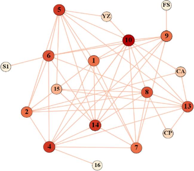
Figure 2. Beijing URTIT network. |
Figure 2 shows the connected directed network with no isolated points. The numbers or letters correspond one−to−one with urban rail transit lines. The deeper the color of a node, the greater its degree, and the more neighboring nodes it has. The colors of node 16, node FS, and node S1 are the lightest because Line 16, Line S1, and FS Line all have interchange relationships with only one line. Differently, Node 10 has the deepest color. Its degree is 11, which means that Line 10 has the interchange relationship with 11 lines.
Using the gray correlation coefficients among different nodes as the edge weight of the Beijing URTIT network, as shown in figure 3.
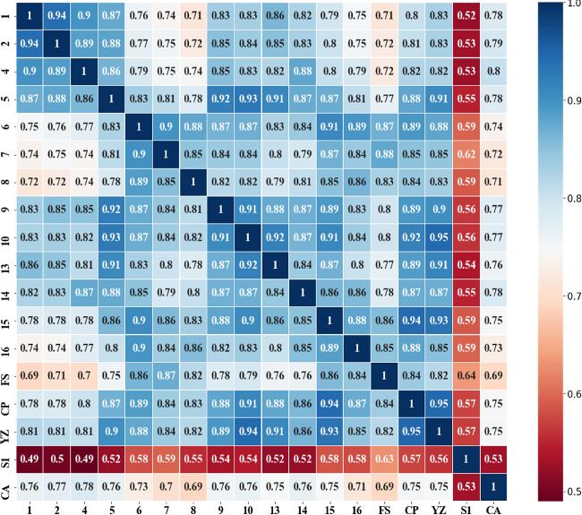
Figure 3. Gray correlation coefficients. |
Different nodes in the network have certain correlations, but there are differences in the extent of correlation. The overall performance of the gray correlation coefficients is acceptable. From figure 3, it can be seen that the range of edge weights is [0.49, 1.00], and the maximum value of edge weights except for the diagonal is 0.95.
4.3. Analysis of a single line
Beijing Subway Line S1 is the second low and medium−speed maglev line in China and the first in Beijing, so we used it as an example to explore the impact of applying new technologies on passenger travel behavior of urban rail transit.
4.3.1. Influence range
In this paper, we set a threshold related to the harmonic centrality. We calculate the harmonic centrality of each node in the network, as presented in table 2.
Table 2. The harmonic centrality. |
| Node | Harmonic centrality | Node | Harmonic centrality |
|---|---|---|---|
| Node 1 | 0.69 | Node 13 | 0.72 |
| Node 2 | 0.70 | Node 14 | 0.76 |
| Node 4 | 0.76 | Node 15 | 0.59 |
| Node 5 | 0.75 | Node 16 | 0.45 |
| Node 6 | 0.74 | Node FS | 0.43 |
| Node 7 | 0.70 | Node CP | 0.50 |
| Node 8 | 0.72 | Node YZ | 0.52 |
| Node 9 | 0.70 | Node S1 | 0.44 |
| Node 10 | 0.82 | Node CA | 0.56 |
As can be seen from table 2, Node 10 has the largest value of harmonic centrality. It indicates that Node 10 is the most central node in the network and Line 10 plays the most important role. The average harmonic centrality of all nodes in the Beijing URTIT network can be expressed as $\bar{p}=0.64$. The threshold can be expressed as $\theta =0.64\,l$, and $l$ is an adjustable parameter. Different results can be obtained by adjusting the parameter $l$. In this section, we will mainly present a series of results when $l=0$. When the parameter $l$ is 0, the threshold $\theta $ is also 0. The influence range is presented in figure 4.
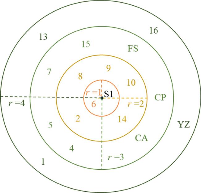
Figure 4. The influence range from Node S1. |
In figure 4, we take Line S1 as the center of the circle. When $r=1$, there are two nodes in the influence area along with the circle center. And when $r=4$, there are all nodes in the influence range. According to figure 4, it can be intuitively seen that the influence range increases with the increase of the influence radius. Furthermore, the influence range and influence ratio are summarized in table 3.
Table 3. The influence range and influence ratio. |
| $r$ | Influence range | $\alpha $ | $\eta $ |
|---|---|---|---|
| 1 | Node 6, S1 | 2 | 11.11% |
| 2 | Node 2, 6, 8, 9, 10, 14, S1 | 7 | 38.89% |
| 3 | Node 2, 4, 5, 6, 7, 8, 9, 10, 14, 15, FS, CP, S1, CA | 14 | 77.78% |
| 4 | Node 1, 2, 4, 5, 6, 7, 8, 9, 10, 13, 14, 15, 16, FS, CP, YZ, S1, CA | 18 | 100% |
Within a certain scope, $\alpha $ and $\eta $ increase as $r$ increases, which indicates that the number of active nodes and the influence ratio increase with the influence radius. In this case, as $r$ gradually increases from 1 to 4, $\alpha $ also increases from 2 to 18 and $\eta $ increases from 11.11% to 100%.
4.3.2. Influence propagation path
The influence propagation path is determined as described in section 3.3.2 . We use Line S1 as the example to find the influence propagation paths. And the ultimate influence propagation paths starting from Node S1 are presented in figure 5.
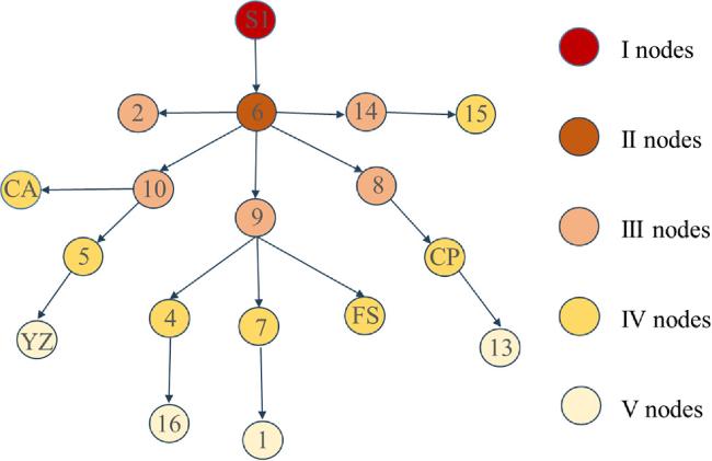
Figure 5. The influence propagation path starting from Node S1. |
Figure 5 contains all the 18 nodes. From figure 5, it can be seen that the influence of Node S1 can reach all nodes in the network. There are five types of nodes with colors ranging from deep to light, namely I nodes, II nodes, III nodes, IV nodes, and V nodes. The path length corresponding to these five types of nodes ranges from 0 to 4. In this case, the maximum path length is 4, indicating that a maximum of 4 transfers are required in the network. The detailed path length is shown in table 4.
Table 4. The path length from Node S1 to other nodes. |
| Node | Path length | Node | Path length | Node | Path length |
|---|---|---|---|---|---|
| Node 1 | 4 | Node 8 | 2 | Node 16 | 4 |
| Node 2 | 2 | Node 9 | 2 | Node FS | 3 |
| Node 4 | 3 | Node 10 | 2 | Node CP | 3 |
| Node 5 | 3 | Node 13 | 4 | Node YZ | 4 |
| Node 6 | 1 | Node 14 | 2 | Node S1 | 0 |
| Node 7 | 3 | Node 15 | 3 | Node CA | 3 |
It is necessary to explain the path length, influence radius, and influence range. It can be understood as the following example. If the influence radius $r=3$, the influence range will include all the influenced nodes with path lengths $d=1$, $d=2$ and $d=3$.
It is to be noted that Node S1 can only be directly propagated to Node 6. The reason is that Line 6 is the only line that has an interchange relationship with Line S1 (opened on December 31, 2017). Figure 6 shows the change in average daily passenger volume of Line 6.
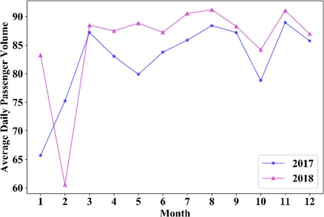
Figure 6. Average daily passenger volume of Line 6. |
It can be seen that the overall passenger volume of Line 6 in 2018 is higher than in 2017, which reflects that the application of new technologies affects the passenger route choice. At the same time, this contrast shows that the application of new technologies changes passenger mode, which makes some passengers switch from other modes to take Line 6 of urban rail transit. In figure 6, the anomalous trend in January and February is due to the different dates of the Spring Festival, in January 2017 and February 2018, respectively. During the Spring Festival, a large number of people return to their hometowns or travel out, which causes urban commuting to plummet.
4.3.3. Influence intensity
There are both positive and negative numbers in the results of $\bigtriangleup {v}_{i}$, which indicate that the passenger volume of some lines increased during the period from January 2018 to December 2020, while the passenger volume of some lines decreased. In this paper, we quantify the influence intensity based on the IPG model. This paper describes the influence intensity of Node S1 on other nodes using the force of gravity $F$, which is presented in figure 7.
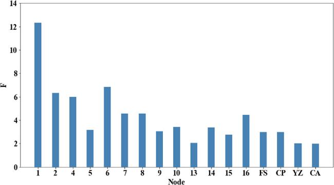
Figure 7. The force of gravity. |
The influence intensity of Node S1 on any other node is also based on the influence propagation path between the two, which reflects the importance of this path. We rank the paths in descending order of the influence intensity, the results are shown in table 5.
Table 5. The order of the influence intensity. |
| Order | Node | Path | $F$ |
|---|---|---|---|
| 1 | Node 1 | S1, 6, 9, 7, 1 | 12.33 |
| 2 | Node 6 | S1, 6 | 6.84 |
| 3 | Node 2 | S1, 6, 2 | 6.33 |
| 4 | Node 4 | S1, 6, 9, 4 | 6.00 |
| 5 | Node 8 | S1, 6, 8 | 4.57 |
| 6 | Node 7 | S1, 6, 9, 7 | 4.55 |
| 7 | Node 16 | S1, 6, 9, 4, 16 | 4.46 |
| 8 | Node 10 | S1, 6, 10 | 3.40 |
| 9 | Node 14 | S1, 6, 14 | 3.37 |
| 10 | Node 5 | S1, 6, 10, 5 | 3.16 |
| 11 | Node 9 | S1, 6, 9 | 3.05 |
| 12 | Node CP | S1, 6, 8, CP | 2.99 |
| 13 | Node FS | S1, 6, 9, FS | 2.96 |
| 14 | Node 15 | S1, 6, 14, 15 | 2.77 |
| 15 | Node 13 | S1, 6, 8, CP, 13 | 2.07 |
| 16 | Node YZ | S1, 6, 10, 5, YZ | 2.00 |
| 17 | Node CA | S1, 6, 10, CA | 1.97 |
The influence intensity of Node S1 on Node 1 is 12.33, which is the largest value, and the influence starts from Line S1 and passes through Line 6, Line 9, Line 7, and Line 1 in sequence. It means that this propagation path plays the most important role. The main reason is that the passenger volume and changes along the path are relatively large, and the transfer time is relatively short. On the contrary, the influence intensity of Node S1 on Node CA is 1.97, which is the smallest value. Its influence propagation path is Line S1, Line 6, Line 10, and Line CA. The main reason is that the passenger volume and its changes along the path are relatively small, and the transfer time is relatively long.
After considering the rationality of the indicator and the availability of data, the average daily passenger intensity and the average daily interchange volume of urban rail transit in Beijing are chosen. Changes in the two indicators reflect the differences in the effects on the lines resulting from the application of new technologies to some extent, which indicates its influence. In this paper, we put forward F for the purpose of reflecting the influence intensity of a particular line equipped with the new technology on other lines. We perform the Spearman correlation analysis with F and the change in the two indicators. The calculated results of the hypothesis testing are shown in table 6.
Table 6. The results of the hypothesis testing. |
| Indicator | Spearman correlation coefficient | P-value |
|---|---|---|
| Daily passenger intensity | 0.6299 | 0.0067 |
| Daily interchange volume | 0.5956 | 0.0116 |
When the significance level is 0.05, the p-values of both indicators are less than it. It means that F and the average daily passenger intensity of urban rail transit in Beijing are correlated, F and the average daily interchanges of urban rail transit in Beijing are correlated, too. The amount of change in both indicators reflects the influence intensity of Line S1 applying new technologies on other lines to some extent. The consistency between F and the realistic indicators illustrates that F can reflect the influence intensity. In other words, the obtained F is reasonable and the proposed model is valid.
4.3.4. Sensitivity analysis on the parameter $l$
This section continues to use Line S1 as the case and conducts sensitivity analysis on the parameter $l$. Based on the special case of $l=0$ shown in section 4.3 , this section will discuss all cases. The window size is set to 0.05.
Case 1 $0\leqslant l\leqslant 0.90$
As mentioned earlier, the rule designed in this paper is to retain edges with edge weights greater than the threshold. The smaller the threshold, the more difficult it is to play a restrictive role. Therefore, it is possible that the threshold does not work within a certain scope. After calculation, we found that when $0\leqslant l\leqslant 0.90$, i.e. $0\leqslant \theta \leqslant 0.58$, the calculation results are all the same. The specific results can be found in section 4.3 , which will not be restated here.
In addition, we need to declare that the basic reason for this situation is that when $0\leqslant \theta \leqslant 0.58$, the edges retained in the global network are the same, with 104 edges.
Case 2 $l\geqslant 0.95$
Line S1 has magnetic levitation technology, but it is located in a remote location and has low passenger capacity. If $l\geqslant 0.95$, then $\theta \geqslant 0.61$. Relative to the value of the threshold, the corresponding edge weights are small. According to the rules, all edges of Node S1 are eliminated, and the influence cannot be propagated. In this case, the influence range, the influence propagation paths, and the influence intensity are meaningless. This is mainly because when $\theta \geqslant 0.61$, the retained edges in the network are non−connected, and the influence cannot propagate outward from Node S1.
We summarize the relationship between the parameter $l$ and the number of edges connected to Node S1, as shown in figure 8.
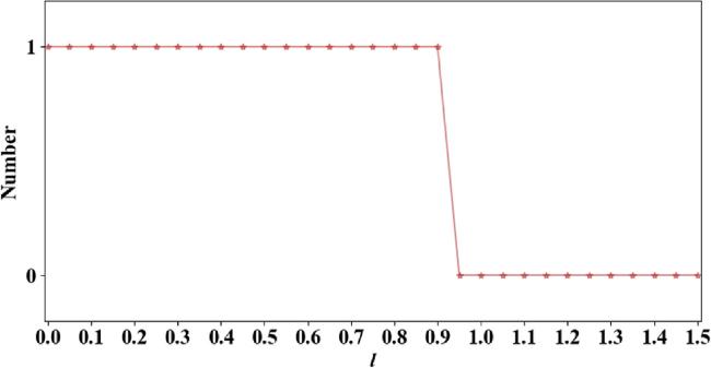
Figure 8. Parameter $l$ and the number of edges connected to Node S1. |
Figure 8 represents the relationship between the threshold $\theta $ and the number of edges connected to Node S1, as the threshold $\theta $ corresponds one−to−one with the parameter $l$.
4.4. Analysis of all lines
In this paper, randomness can be interpreted as chance or serendipity. If only one line in Beijing URTIT Network is investigated, the results will only be based on this particular line. In other words, the results are likely to be individualized rather than generalized. In order to avoid randomness, we will explore all lines in the Beijing URTIT network in this section.
4.4.1. Influence range
In this section, the influence radius is still used to depict the influence range. As the influence radius increases, the influence gradually spreads outward from the circle center, and the influence range gradually expands. When the parameter $l=0$, we consider the case of all lines and draw a schematic diagram of the influence range as shown in figure 9.
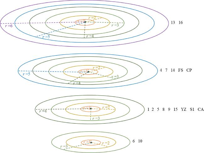
Figure 9. The influence range. |
The maximum influence radius ranges from 3 to 6. Line 13 and Line 16 have the largest influence radius. It means that from Line 13 or Line 16, there exist lines that require six transfers to get there. Line 4, Line 7, Line 14, FS Line, and CP Line have a maximum influence radius of 5. From these lines, there are lines in the network that require five transfers. Similarly, lines with a maximum influence radius of 4 include Lines 1, Line 2, Line 5, Line 8, Line 9, Line 15, YZ Line, Line S1, and CA Express, which means that they require up to four transfers. Lines 6 and 10 only require a maximum of three transfers.
4.4.2. Influence propagation path
We counted the lengths of all influence propagation paths in the network and calculated the percentage of different path lengths. Figure 10 shows the number and proportion of different path lengths.
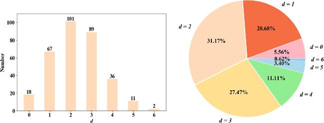
Figure 10. The number and proportion of different path lengths. |
A path length of 0 indicates a node to itself. There are 18 nodes in total, so there are 18 paths with length 0. In this case, the maximum path length is 6, indicating that a maximum of six transfers are required in the network. But there are only two paths of length 6. The path length of 2 has the highest percentage, accounting for about one−third of the total. In addition, the proportion of path lengths of 1 and 3 is also high, both exceeding 20%. Obviously, path lengths of 1, 2, and 3 account for more than three−quarters of the total. While the proportion of path lengths of 4 is about 11%. The proportion of 5 is only a little more than 3%. It is reasonable considering the situation of actual interchanges.
4.4.3. Influence Intensity
The IPG model is used to measure the influence intensity. Specifically, the force of gravity $F$ is determined by the average daily passenger volume per month ${\rm{\Delta }}v$, transfer time $t$, and distance $d$. All the forces of gravity $F$ are shown in figure 11.
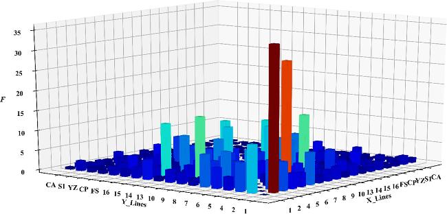
Figure 11. The number and proportion of different path lengths. |
The $F$ value from Line 2 to Line 1 is the highest, exceeding 35, which is largely due to the large average daily passenger volume of Node 1 and Node 2 per month. The path length from Line 2 to Line 1 is 1, which also reflects its short transfer time to a certain extent. Transfer time only takes about 30 s. On average, the $F$ values of Line 1, Line 2, Line 4, Line 6, Line 7, Line 9, and Line 10 are relatively high. They all have an average $F$ value of more than 3. The main reason is that these lines themselves have a larger average daily passenger volume per month and have shorter transfer times and path lengths. Comparatively speaking, Line 13, Line 15, Line 16, YZ Line, and CA Express have small $F$ values, and their average $F$ values are less than 1. This is due to the fact that their average daily passenger volume per month is smaller and their transfer times and path lengths are not as short. Overall, the results correspond to the actual situation and show the rationality of our proposed method.
4.4.4. Sensitivity analysis on the parameter $l$
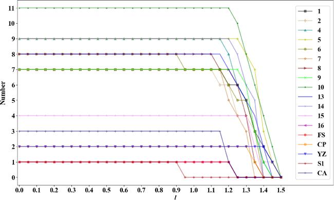
The calculated average harmonic centrality is 0.64, and the value of the threshold $\theta $ is $0.64l$. If $\theta $ is not large enough, it may have a limited restricting effect when compared with edge weights. In fact, the parameter $l$ determines the threshold $\theta $. Therefore, it is necessary to explore the relationship between the parameter $l$ and the number of edges connected to each node in the network. The relationship is shown in figure 12.
Figure 12. The parameter $l$ and the number of connected edges. |
Figure 12 summarizes the relationship between the parameter $l$ and the number of connected edges of all nodes. In general, the larger $l$ is, the fewer edges there are. When $l$ is between 0 and 0.90, all nodes have the same number of edges, and then changes, especially when $l$ is greater than 1.10, the change is obvious, until $l$ is 1.50, there are no edges in the network.
5. Conclusions
Urban rail transit has become one of the most important modes of public transport after decades of development. It cannot be achieved without the updating and application of technologies. Obviously, new technologies of urban rail transit can affect passenger travel behavior. From a holistic point of view, this paper considers lines of urban rail transit as nodes to construct the URTIT network. In the network, the interchange relationship among lines is the basis for edges, and the gray correlation coefficient is used as the edge weight.
We investigate an influence propagation mechanism including the influence range, the influence propagation path, and the influence intensity. The influence propagation mechanism is inseparable from the threshold that is set as the average harmonic centrality of all nodes in the network. The influence radius proposed in this paper can assist in explaining the influence range. The number of active nodes and the influence ratio increase with the influence radius, the influence range naturally expands as well. The determination of the influence propagation paths is based on the application of the Dijkstra algorithm considering time and distance, and we proposed the IPG model for measuring the influence intensity $F$. The values reflect the average daily passenger volume per month, transfer time, and distance of lines.
This paper develops a case study of Beijing, China. On the one hand, Beijing Subway Line S1 is used as an example. On the other hand, we analyze all the lines of the Beijing URTIT network to avoid randomness. The maximum influence radius ranges from 3 to 6, and the maximum radius of Line S1 is 4. The number and proportion of different path lengths are visualized, with more than three−quarters of the lengths being 1, 2, and 3. And the influence intensity is determined by the passenger volume, transfer time, and distance. In this paper, we not only demonstrate the influence range, influence propagation path, and influence intensity, but also analyze the relationship between the parameter $l$ and the number of connected edges. The research results of this paper are consistent with reality.
In this paper, we explore passenger travel behavior in urban rail transit based on the networked model from the macro level. Therefore, the specific passenger mode and route choice of individual passengers are not considered. Moreover, currently limited by the insufficiency of detailed data on passenger mode and route choice, we would like to add related research at the micro level in the future.