In this paper, we investigate the integrable fractional coupled Gerdjikov–Ivanov equation and derive its explicit form by employing the completeness relation of squared eigenfunctions. Based on the Riemann–Hilbert method, we construct the fractional N-soliton solutions. We find that as the power ε of the Riesz fractional derivative increases, the amplitudes of the fractional soliton solutions remain invariant, while their widths decrease and the absolute values of the wave velocity, group velocity, and phase velocity increase. Additionally, we examine the long-time asymptotic behavior of the fractional N-soliton solution. The results show that as t →±∞, the solution can be approximated by the sum of N fractional one-soliton solutions, with each soliton's amplitude and velocity remaining constant, whereas both position and phase shifts are observed.
Xiaoqian Huang, Huanhe Dong, Yong Zhang. The N-soliton solution and its asymptotic analysis of the fractional coupled Gerdjikov–Ivanov equation[J]. Communications in Theoretical Physics, 2025, 77(12): 125002. DOI: 10.1088/1572-9494/adeb5a
1. Introduction
Exploring fractional integrable nonlinear equations and their exact solutions is an active topic in many fields [1]. These equations typically provide better reflections of various nonlinear phenomena in mathematical, physical, and biological systems, among others. Numerous fractional derivatives have been introduced to more precisely describe complex mathematical models, including the Caputo–Fabrizio fractional derivative [2], the Atangana–Baleanu fractional derivative [3] and the time fractional conformable derivative [4, 5]. Physical models with fractional derivatives in fields including fluid mechanics [6, 7], plasma physics [8, 9] and nonlinear optics [10, 11] exhibit considerable promise for a wide array of advanced applications. In particular, the fractional nonlinear Schrödinger (NLS) equation serves as a fundamental model for describing soliton propagation in optical fibers [12, 13]. Furthermore, fractional derivatives possess the significant capability of modeling various real-world phenomena that exhibit memory effects, making them particularly relevant to a wide range of biological systems. Hence, they provide a valuable framework for modeling and analyzing the rheological properties of cells and the electrical conductance of cell membranes in biological systems [14].
In 2022, Ablowitz, Been, and Carr introduced integrable fractional nonlinear equations related to the Riesz fractional derivative [15]. The introduction of Riesz fractional derivatives established a link between fractional calculus and Fourier transforms [16] and it represents a fractional extension of the negative of second derivative (i.e., ${\left|-{\partial }_{x}^{2}\right|}^{\epsilon }$, where ε ∈ [0, 1)). For any sufficiently smooth function f(x), ${\left|-{\partial }_{x}^{2}\right|}^{\epsilon }f(x)$ can be expressed as ${{ \mathcal F }}^{-1}({\left|k\right|}^{2\epsilon }{ \mathcal F }f(x))$, where ${ \mathcal F }$ denotes the Fourier transform, ${{ \mathcal F }}^{-1}$ indicates the inverse Fourier transform, and ${\left|k\right|}^{2\epsilon }$ for $k\in {\mathbb{R}}$ represents the spectrum of the operator. Then the new forms for the fractional NLS equation, the fractional Korteweg–de Vries (KdV) equation, the fractional Sine–Gordon equation and the fractional modified Korteweg–de Vries (mKdV) equation were first obtained [15, 17]. In particular, these fractional nonlinear equations are integrable because of their Lax pair and fractional recursion operator. This property ensures that they also possess the soliton solutions and the infinite conservation law. Subsequently, construction methods of fractional integrable nonlinear equations related to the Riesz fractional derivative in [15] were further extended, and related research results emerged. In [18, 19], Yan et al investigated the fractional higher-order NLS equation using this approach and obtained their fractional solutions through the inverse scattering transform (IST), discovering that these fractional solitons also exhibit anomalous dispersion phenomena. Then, in terms of the power of the Riesz fractional derivative, they proposed an innovative idea, introducing integrable multi-Lévy-index and mix-Lévy-index fractional nonlinear equations [20]. In [21], An et al studied the integrable fractional coupled Hirota equation and presented its N-soliton solution using the IST.
However, the aforementioned integrable fractional equations are inherently associated with the Ablowitz–Kaup–Newell–Segur (AKNS) system. Taking higher-order nonlinear effects into account, the derivative nonlinear Schrödinger (DNLS) equations with a polynomial spectral problem of arbitrary order are investigated. These equations have a broad physical background, including weakly nonlinear dispersive water waves [22], quantum field theory [23], and plasmas [24, 25]. There exist three well-known DNLS equations, namely: the DNLS I equation [26]
also known as the Gerdjikov–Ivanov (GI) equation [30]. These three equations are known to belong to the KN system and can be transformed into each other by means of a gauge transformation. By employing equation (2.12) in [31], DNLS II equation can be transformed into the DNLS I equation. Subsequently, by integrating equation (3), equation (4) and equation (6) with γ = 0 in [32], the DNLS I equation can be converted into the DNLS III equation. In recent years, several solutions of the one-component GI equation have been proposed, such as the soliton solutions [33], the algebra-geometric solution [34], and the Wronskian type solution [35]. In contrast to one-component systems, multi-component systems demonstrate more intricate dynamical behaviors and are capable of modeling more complex physical phenomena. The vector form of the GI equation is as follows:
where qj ≡ qj(x, t)(j = 1, 2, ⋯ , n) and the superscript † indicates the Hermitian conjugate of a vector. When n = 2, the integrable coupled GI (CGI) equation is derived
For equation (2), Zhang, Cheng, and He derived its N-soliton solutions by utilizing the matrix Riemann–Hilbert (RH) problem [36]. The IST is a widely used and effective method, which was originally introduced to solve the initial value problems for nonlinear integrable evolution equations. The classical IST is related to the Gel'fand–Levitan–Marchenko (GLM) integral equations [37, 38]. In the 1970s, the RH method was proposed by Novikov et al [39], which significantly simplified the classical IST method and found extensive applications. For instance, when dealing with second-order spectral problems, the GLM equations are effectively equivalent to RH problems. However, for higher-order spectral problems, this equivalence does not hold true. In these cases, it becomes imperative to convert the inverse scattering part into a RH problem for a comprehensive analysis. This work centers on examining the integrable fractional extension of the CGI equation and employ the RH method to derive exact fractional solutions of the integrable fractional CGI (FCGI) equation.
This paper is organized as follows. In section 2, the anomalous dispersion relation and the fractional function ${{ \mathcal F }}_{FG}({ \mathcal N })$ are derived. In section 3, we construct the RH problem as well as provide its solution via using the Plemelj formula. Additionally, we present the explicit form of the FCGI equation in section 4. In section 5, the N-soliton solutions of the FCGI equation are provided. Subsequently, we investigate the long-time asymptotic behavior of the fractional N-soliton solutions. The last section is our conclusions.
2. The anomalous dispersion relation
In this section, from the Lax pair of the CGI equation and the zero curvature equation, we find the dispersion relation of the CGI equation and the function ${{ \mathcal F }}_{G}({ \mathcal N })$ with the recursive operator ${ \mathcal N }$. Then, by considering the dispersion relation, the anomalous dispersion relation for the FCGI equation and the function ${{ \mathcal F }}_{FG}({ \mathcal N })$ with the recursive operator ${ \mathcal N }$ are obtained.
The Lax pair of the CGI equation is given as follows
with the spectral parameter $\zeta \in {\mathbb{C}}$. Y ≡ Y(ζ; x, t) is a 3 × 3 matrix function, qj (j = 1, 2) are potential functions, V11 is a scalar function, ${{{\boldsymbol{V}}}_{12}}^{\top }$ and V21 are 2-dimensional column vectors, and V22 is a 2 × 2 matrix. Then, by calculating the zero curvature equation
with $\partial =\frac{\partial }{\partial x}$ being a differential operator. Assume that ${V}_{11}^{0}$, ${{\boldsymbol{V}}}_{22}^{0}$, ${{{\boldsymbol{V}}}_{12}}^{\top }$ and V21 are polynomials of ζ
Furthermore, by inserting equations (9) and (10) into equation (8) and matching the coefficients of each power of ζ, we derive the following set of recurrence relations
$\begin{eqnarray*}\begin{array}{rcl}{\left[\begin{array}{c}{{\boldsymbol{q}}}^{\top }\\ -{{\boldsymbol{q}}}^{\dagger }\end{array}\right]}_{t} & = & {{ \mathcal N }}_{1}{{ \mathcal N }}_{2}\left[\begin{array}{c}{{{\boldsymbol{b}}}^{[n]}}^{\top }\\ {{\boldsymbol{c}}}^{[n]}\end{array}\right],\,\left[\begin{array}{c}{{{\boldsymbol{b}}}^{[1]}}^{\top }\\ {{\boldsymbol{c}}}^{[1]}\end{array}\right]=-2{{{ \mathcal N }}_{3}}^{-1}\left[\begin{array}{c}{{\boldsymbol{q}}}^{\top }\\ {{\boldsymbol{q}}}^{\dagger }\end{array}\right],\\ \left[\begin{array}{c}{{{\boldsymbol{b}}}^{[j]}}^{\top }\\ {{\boldsymbol{c}}}^{[j]}\end{array}\right] & = & \frac{1}{2{\rm{i}}}{{{ \mathcal N }}_{3}}^{-1}{{ \mathcal N }}_{1}{{ \mathcal N }}_{2}\left[\begin{array}{c}{{{\boldsymbol{b}}}^{[j-1]}}^{\top }\\ {{\boldsymbol{c}}}^{[j-1]}\end{array}\right],\,j\geqslant 2.\end{array}\end{eqnarray*}$
Therefore, the CGI integrable hierarchies can be found,
$\begin{eqnarray}\begin{array}{rcl}{\left[\begin{array}{c}{{\boldsymbol{q}}}^{\top }\\ -{{\boldsymbol{q}}}^{\dagger }\end{array}\right]}_{t} & = & -4{\rm{i}}{ \mathcal F }({ \mathcal N })\left[\begin{array}{c}{{\boldsymbol{q}}}^{\top }\\ -{{\boldsymbol{q}}}^{\dagger }\end{array}\right],\\ { \mathcal F }\left({ \mathcal N }\right) & = & {{ \mathcal N }}^{n},\quad { \mathcal N }=\frac{1}{2{\rm{i}}}{{ \mathcal N }}_{1}{{ \mathcal N }}_{2}{{{ \mathcal N }}_{3}}^{-1}.\end{array}\end{eqnarray}$
Next, according to the linearized form of equation (11)
$\begin{eqnarray}\begin{array}{rcl}{\left[\begin{array}{c}{{\boldsymbol{q}}}^{\top }\\ -{{\boldsymbol{q}}}^{\dagger }\end{array}\right]}_{t} & = & -4{\rm{i}}{ \mathcal F }\left(\frac{1}{2{\rm{i}}}{{ \mathcal N }}_{0}\right)\left[\begin{array}{c}{{\boldsymbol{q}}}^{\top }\\ -{{\boldsymbol{q}}}^{\dagger }\end{array}\right],\\ { \mathcal F }\left(\frac{1}{2{\rm{i}}}{{ \mathcal N }}_{0}\right) & = & {\left(\frac{1}{2{\rm{i}}}{{ \mathcal N }}_{0}\right)}^{n},\\ {{ \mathcal N }}_{0} & = & {\mathrm{diag}}(\partial ,\partial ,-\partial ,-\partial ),\end{array}\end{eqnarray}$
and inserting it into the linearization equation equation (13), the dispersion relation can be yielded
$\begin{eqnarray}{\gamma }_{l}\left({\zeta }_{l}\right)=4{\left(\frac{{\zeta }_{l}}{2}\right)}^{n}=4{ \mathcal F }\left(\frac{{\zeta }_{l}}{2}\right),\quad l=1,2.\end{eqnarray}$
When n = 2, the dispersion relation of the CGI equation is ${\gamma }_{G,j}\left({\zeta }_{j}\right)={{\zeta }_{j}}^{2}$, and the function related to the recursive operator ${ \mathcal N }$ is ${{ \mathcal F }}_{G}\left({ \mathcal N }\right)={{ \mathcal N }}^{2}$. Based on the dispersion relation ${\gamma }_{G,j}\left({\zeta }_{j}\right)$, the anomalous dispersion relation of the FCGI equation can be expressed as ${\gamma }_{FG,j}\left({\zeta }_{j}\right)={{\zeta }_{j}}^{2}{\left|{\zeta }_{j}\right|}^{\epsilon }$, ε ∈ [0, 1). Accordingly, we obtain the linearized expression of the FCGI equation as
Hence, the fractional operator of the FCGI equation is
$\begin{eqnarray}{{ \mathcal F }}_{FG}({ \mathcal N })={{ \mathcal N }}^{2}{\left|2{ \mathcal N }\right|}^{\epsilon },\quad \epsilon \in [0,1).\end{eqnarray}$
3. Riemann–Hilbert method
In this section, we will explore the RH method for the FCGI equation and present the reconstruction formula for the potential functions q1(x, t) and q2(x, t). This procedure is carried out through both the direct and inverse scattering processes.
3.1. The direct scattering
Similar to other fractional integrable equations, the time part V(ζ;x, t) of the Lax pair for the integrable FCGI equation cannot be explicitly written out. Therefore, we assume that the potential function q(x, t) is sufficiently smooth and rapidly decays to zero as x → ±∞, and the following asymptotic behavior is given
$\begin{eqnarray}{\boldsymbol{V}}\to \left[\begin{array}{cc}-2{\rm{i}}{{ \mathcal F }}_{FG}({\zeta }^{2}) & {\bf{0}}\\ {\bf{0}} & 2{\rm{i}}{{ \mathcal F }}_{FG}({\zeta }^{2}){{\mathbb{I}}}_{2}\end{array}\right],\quad x\to \pm \infty .\end{eqnarray}$
Then the Lax pair of the integrable FCGI equation can be written as
where matrix V satisfies the asymptotic behavior in equation (19).
First, we treat the time variable t as a formal parameter and focus on the spectral properties of the spatial part of the Lax pair. In terms of the Lax pair equation (20), we obtain the Jost solutions
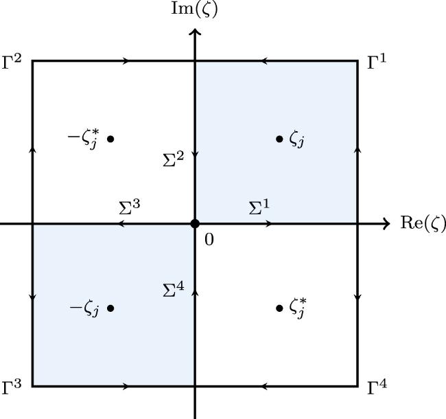
where ${{\rm{e}}}^{\alpha \widehat{{\boldsymbol{\sigma }}}}{\boldsymbol{A}}={{\rm{e}}}^{{\boldsymbol{\alpha }}{\boldsymbol{\sigma }}}{\boldsymbol{A}}{{\rm{e}}}^{-\alpha {\boldsymbol{\sigma }}}$ with A being a 3 × 3 matrix and α being a scalar variable. We note that, as long as the integrals on the right sides of the Volterra integral equations converge, ${{\boldsymbol{J}}}_{\pm }=\left[\begin{array}{ccc}{{\boldsymbol{J}}}_{\pm }^{[1]} & {{\boldsymbol{J}}}_{\pm }^{[2]} & {{\boldsymbol{J}}}_{\pm }^{[3]}\end{array}\right]$ allow for analytical continuation off ${\rm{\Sigma }}={\mathbb{R}}\cup {\rm{i}}{\mathbb{R}}$. A brief analysis reveals that the exponential factor ${{\rm{e}}}^{2{\rm{i}}{\zeta }^{2}(x-y)}$ plays a major role in the integral equation for ${{\boldsymbol{J}}}_{-}^{[1]}$. Since y < x in the integral, ${{\rm{e}}}^{2{\rm{i}}{\zeta }^{2}(x-y)}$ decays rapidly when ζ lies in ${{\rm{\Omega }}}^{+}=\left\{\zeta \left|\,\arg \zeta \in \left(0,\frac{\pi }{2}\right)\cup \left(\pi ,\frac{3\pi }{2}\right)\right.\right\}$. Similarly, the integral equations for ${{\boldsymbol{J}}}_{+}^{[2]}$ and ${{\boldsymbol{J}}}_{+}^{[3]}$ involve only the exponential factor ${{\rm{e}}}^{-2{\rm{i}}{\zeta }^{2}(x-y)}$, and since y > x in these integrals, ${{\rm{e}}}^{-2{\rm{i}}{\zeta }^{2}(x-y)}$ also decays when ζ lies in Ω+. Hence, $\left[\begin{array}{ccc}{{\boldsymbol{J}}}_{-}^{[1]} & {{\boldsymbol{J}}}_{+}^{[2]} & {{\boldsymbol{J}}}_{+}^{[3]}\end{array}\right]$ are analytic for ζ ∈ Ω+ and continuous for ζ ∈ Ω+ ∪ Σ. In contrast, $\left[\begin{array}{ccc}{{\boldsymbol{J}}}_{+}^{[1]} & {{\boldsymbol{J}}}_{-}^{[2]} & {{\boldsymbol{J}}}_{-}^{[3]}\end{array}\right]$ are analytic for $\zeta \in {{\rm{\Omega }}}^{-}=\left\{\zeta \left|\,\arg \zeta \in \left(\frac{\pi }{2},\pi \right)\cup \left(\frac{3\pi }{2},2\pi \right)\right.\right\}$ and continuous for ζ ∈ Ω− ∪ Σ, as shown explicitly in figure 1.
Figure 1. Complex ζ-plane. The blue and white parts illustrate Ω+ and Ω−, respectively. The arrow directions along the blue regions represent Σ+ = (Σ2 + Σ1) + (Σ4 + Σ3), Γ+ = Γ1 + Γ3. The arrow directions along the white regions represent Σ− = (Σ2 + Σ3) + (Σ4 + Σ1), Γ− = Γ2 + Γ4. Furthermore, Σ = Σ+ + Σ−.
In addition, taking into account that ${{\boldsymbol{J}}}_{\pm }^{-1}={\left[\begin{array}{ccc}{\widetilde{{\boldsymbol{J}}}}_{\pm }^{[1]} & {\widetilde{{\boldsymbol{J}}}}_{\pm }^{[2]} & {\widetilde{{\boldsymbol{J}}}}_{\pm }^{[3]}\end{array}\right]}^{\top }$ satisfy the adjoint equation of equation (23), that is,
through a similar analysis as above, we can find that ${\left[\begin{array}{ccc}{\widetilde{{\boldsymbol{J}}}}_{-}^{[1]} & {\widetilde{{\boldsymbol{J}}}}_{+}^{[2]} & {\widetilde{{\boldsymbol{J}}}}_{+}^{[3]}\end{array}\right]}^{\top }$are analytic for ζ ∈ Ω− and continuous for ζ ∈ Ω− ∪ Σ. Conversely, ${\left[\begin{array}{ccc}{\widetilde{{\boldsymbol{J}}}}_{+}^{[1]} & {\widetilde{{\boldsymbol{J}}}}_{-}^{[2]} & {\widetilde{{\boldsymbol{J}}}}_{-}^{[3]}\end{array}\right]}^{\top }$are analytic for ζ ∈ Ω+ and continuous for ζ ∈ Ω+ ∪ Σ.
Next, in order to clarify the calculation process, we replace the Jost solutions Y+, Y− with $\Psi$, Φ, representing them as collections of column vectors, while their inverse matrices $\Psi$−1, Φ−1 are represented as collections of row vectors
Based on the analytic properties of modified Jost solutions J± and ${{\boldsymbol{J}}}_{\pm }^{-1}$, we present the analytic properties of the Jost solutions $\Psi$ and Φ, as well as those of their inverse matrix $\Psi$−1 and Φ−1
where the superscripts ‘±' designate the domain of analyticity for the corresponding quantity.
Since both $\Psi$ and Φ are solutions to the Lax pair equation (20), there exists a scattering matrix ${\boldsymbol{S}}\equiv {\boldsymbol{S}}(\zeta ;t)\,={({s}_{ij}(\zeta ;t))}_{3\times 3}$, such that
where $|\,\cdot ,\cdot |$ denotes the determinant. According to the analytic properties of Jost solutions in equation (28), the analytic properties of the scattering data are provided
where the superscripts ‘±' represents that the scattering data are analytic on the complex plane Ω±, respectively. However, the scattering data ${s}_{1j},\,{s}_{j1},\,{\tilde{s}}_{1j}$ and ${\tilde{s}}_{j1}$ (j = 2, 3) do not generally permit analytic extensions to Ω±.
After that, from the symmetries σQσ = −Q and Q† = Q, we provide two symmetry properties of J±(ζ; x, t)
which implies that s11(ζ; t) = s11(− ζ;t) = ${\tilde{s}}_{11}^{* }({\zeta }^{* };t)$ = ${\tilde{s}}_{11}^{* }(-{\zeta }^{* };t)$. Suppose that s11 contains 2N simple zeros, expressed as ±ζk(1 ≤ k ≤ N). At the same time, ${\tilde{s}}_{11}$ also possesses 2N simple zeros defined by $\pm {\zeta }_{k}^{* }$(1 ≤ k ≤ N). The zeros ζ = ± ζk and $\zeta =\pm {\zeta }_{k}^{* }$ of s11 and ${\tilde{s}}_{11}$ are also called the discrete spectra of equation (23), respectively. Moreover, the continuous spectra of equation (23) all lie on Σ, which is shown in figure 1.
Next, according to the asymptotic behavior of V in equation (19), the time evolution of the scattering data can be presented
Next, we first analyze the regular RH problem. Based on this, by transforming the irregular RH problem into the regular RH problem, we further derive the reconstruction formulas for the potential functions q1(x, t) and q2(x, t).
For ${\rm{\det }}{{\boldsymbol{K}}}^{+}={s}_{11}\ne 0$ and ${\rm{\det }}{{\boldsymbol{K}}}^{-}={\tilde{s}}_{11}\ne 0$ in their respective domains of analyticity, the RH problem 1 is regular. Then, to facilitate its solution using the Plemelj's formula [41], we rewrite equation (37) as
where Σ± are indicated in figure 1. Consider K± and ${\widehat{{\boldsymbol{K}}}}^{\pm }$ as two sets of solutions to the RH problem 1, which implies that
which indicates the uniqueness of the solution to the regular RH problem 1.
For $\det {{\boldsymbol{K}}}^{+}={s}_{11}=0$ and $\det {{\boldsymbol{K}}}^{-}={\tilde{s}}_{11}=0$ in their respective domains of analyticity, the RH problem 1 is irregular. In this case, the RH problem 1 possesses a unique solution under the condition that the zeros of $\det {{\boldsymbol{K}}}^{+}$ and $\det {{\boldsymbol{K}}}^{-}$ in Ω± are identified, and the kernel structures of K± at these zeros are specified. In the previous subsection, we assumed that s11 and ${\tilde{s}}_{11}$ have 2N simple zeros. Consequently, the kernel of K+(ζk; x, t) comprises a singular column vector $\left|{{\boldsymbol{v}}}_{k}\right\rangle \equiv \left|{{\boldsymbol{v}}}_{k}\right\rangle ({\zeta }_{k};x,t)={\left[\begin{array}{ccc}{\left|{{\boldsymbol{v}}}_{k}\right\rangle }_{1} & {\left|{{\boldsymbol{v}}}_{k}\right\rangle }_{2} & {\left|{{\boldsymbol{v}}}_{k}\right\rangle }_{3}\end{array}\right]}^{\top }$, and the kernel of ${{\boldsymbol{K}}}^{-}\left({\zeta }_{k};x,t\right)$ consists of a singular row vector ${\left|{{\boldsymbol{v}}}_{k}\right\rangle }^{\dagger }=\left[\begin{array}{ccc}{\left|{{\boldsymbol{v}}}_{k}\right\rangle }_{1}^{* } & {\left|{{\boldsymbol{v}}}_{k}\right\rangle }_{2}^{* } & {\left|{{\boldsymbol{v}}}_{k}\right\rangle }_{3}^{* }\end{array}\right]$, that is,
Below, to remove the zero structures in the irregular RH problem 1 and transform it into a solvable regular RH problem 2, we propose the following transformation
and $\left|{{\boldsymbol{z}}}_{k}\right\rangle ={{\boldsymbol{D}}}_{k-1}\left({\zeta }_{k}\right)\cdots {{\boldsymbol{D}}}_{1}\left({\zeta }_{k}\right)\left|{{\boldsymbol{v}}}_{k}\right\rangle $ and $\left\langle {{\boldsymbol{z}}}_{k}\right|$ refers to a row vector.
Then, the matrix functions ${\widetilde{{\boldsymbol{K}}}}^{\pm }$ are subject to the following RH problem 2.
The 3 × 3 matrix functions ${\widetilde{{\boldsymbol{K}}}}^{\pm }$ satisfy following properties
Analyticity: ${\widetilde{{\boldsymbol{K}}}}^{\pm }$ are analytic in Ω±, respectively.
Asymptotic behavior: As ζ → ∞, ${\widetilde{{\boldsymbol{K}}}}^{\pm }$ possess the following asymptotic behavior
Before solving RH problem 2, we first explain the expression of Bk. Since ${\boldsymbol{D}}(\zeta ){{\boldsymbol{D}}}^{-1}(\zeta )={{\mathbb{I}}}_{3}$ holds for any ζ ∈ Ω±, we obtain the following relation
which implies that ${{\boldsymbol{B}}}_{k}^{\dagger }$ must be one-dimensional. Meanwhile, from equation (43) and analytic properties of ${\widetilde{{\boldsymbol{K}}}}^{\pm }$, we have ${\boldsymbol{D}}\left({\zeta }_{k}\right)\left|{{\boldsymbol{v}}}_{k}\right\rangle =0$ and ${\left|{{\boldsymbol{v}}}_{k}\right\rangle }^{\dagger }{{\boldsymbol{D}}}^{-1}\left({\zeta }_{k}^{* }\right)=0$. This indicates that Bk is linearly related to ${\left|{{\boldsymbol{v}}}_{k}\right\rangle }^{\dagger }$. Therefore, Bk can be expressed as equation (47). Furthermore, we express D(ζ) and D−1(ζ) in equations (45) and (46) as the following summation representations
Thus, we can provide the expressions for $\left|{{\boldsymbol{\mu }}}_{k}\right\rangle \,={\left[\begin{array}{ccc}{\left|{{\boldsymbol{\mu }}}_{k}\right\rangle }_{1} & {\left|{{\boldsymbol{\mu }}}_{k}\right\rangle }_{2} & {\left|{{\boldsymbol{\mu }}}_{k}\right\rangle }_{3}\end{array}\right]}^{\top }$from equation (52)
and the elements of ${\boldsymbol{P}}={\left({P}_{ij}\right)}_{N\times N}$ and $\widehat{{\boldsymbol{P}}}={\left({\widehat{P}}_{ij}\right)}_{N\times N}$ are expressed as
Subsequently, we expand the analytic function K+ as ζ → ∞ and provide the reconstruction formula for the potential functions of the FCGI equation. The asymptotic expansion of K+ is given by
$\begin{eqnarray}{{\boldsymbol{K}}}^{+}={{\boldsymbol{K}}}_{0}^{+}+{{\boldsymbol{K}}}_{1}^{+}{\zeta }^{-1}+{{\boldsymbol{K}}}_{2}^{+}{\zeta }^{-2}+{ \mathcal O }\left({\zeta }^{-3}\right),\end{eqnarray}$
where ${{\boldsymbol{K}}}_{j}^{+}(j=1,2,\ldots )$ denote the coefficients of ζ−j, respectively. Substituting it into the equation (23) and equating the coefficients of ζ, this results in
which imply ${{\boldsymbol{K}}}_{0,x}^{+}=0.$ With out loss of generality, we set ${{\boldsymbol{K}}}_{0}^{+}={{\mathbb{I}}}_{3}$, then Q can be expressed as
where ${{\boldsymbol{K}}}_{1}^{+}$ is given explicitly in section 5.
4. The explicit form of the FCGI equation
In this section, we aim to construct the explicit form of the FCGI equation using the square eigenfunctions and their completeness relation.
On one hand, by means of perturbation theory (or variational relations) and a RH problem, we define the squared eigenfunctions and their adjoint squared eigenfunctions, as well as their completeness relations. On the other hand, according to equation (11), we need to analyze the action of ${{ \mathcal F }}_{FG}({ \mathcal N })$ on the potential function ${\left[\begin{array}{cc}{{\boldsymbol{q}}}^{\top } & -{{\boldsymbol{q}}}^{\dagger }\end{array}\right]}^{\top }$. Since the squared eigenfunctions are eigenfunctions of the recursion operator for integrable equations [41], we transform the problem of ${ \mathcal N }$ acting on ${\left[\begin{array}{cc}{{\boldsymbol{q}}}^{\top } & -{{\boldsymbol{q}}}^{\dagger }\end{array}\right]}^{\top }$ into the problem of ${ \mathcal N }$ acting on squared eigenfunctions. This method can also be applied to the fractional operator function ${{ \mathcal F }}_{FG}({ \mathcal N })$.
Consider a perturbation to the spectral problem (20) for the Jost solution Φ
From the asymptotic of J± at large distances, the Jost solution Φ exhibits an asymptotic behavior ${\boldsymbol{\Phi }}\to {{\rm{e}}}^{-{\rm{i}}{\zeta }^{2}{\boldsymbol{\sigma }}x}$ as x → −∞. Consequently, δΦ → 0 as x → −∞. With this boundary condition established, the solution of the inhomogeneous equation (60) is obtained
In addition, considering ${\boldsymbol{\Psi }}\to {{\rm{e}}}^{-{\rm{i}}{\zeta }^{2}{\boldsymbol{\sigma }}x}$ as x → +∞ and scattering relation equation (29), we derive
Nevertheless, $\delta {s}_{1j},\,\delta {s}_{j1},\,\delta {\tilde{s}}_{1j}$ and $\delta {\tilde{s}}_{j1}$ (j = 2, 3) are also not analytic in Ω±. The reflection coefficients are defined as
Taking into account the analytic properties of Jost solutions and scattering matrix, we can conclude that φj are analytic in Ω−, and ${\widetilde{{\boldsymbol{\varphi }}}}_{j}$ are analytic in Ω+. As a consequence, the analytic properties of δρj1 and δσ1j are determined. We rewrite the variation relation equation (68) as
Next, we will present the variational expression of the potential functions represented by the scattering data. From the matrix function K±, we construct two new matrix functions
where δ(x) is the Dirac's delta function and equation (93) is called the completeness relation of the squared eigenfunctions. However, the functions s11 and ${\tilde{s}}_{11}$ possess simple zeros {± ζk}(1 ≤ k ≤ N) and $\{\pm {\zeta }_{k}^{* }\}(1\leqslant k\leqslant N)$. Therefore, when zeros exist, the completeness relation in equation (93) no longer holds. Instead, by applying the residue theorem, it is replaced by the following completeness relation
Since the squared eigenfunctions ${{\boldsymbol{Z}}}_{j1}^{+}$ and ${{\boldsymbol{Z}}}_{1j}^{-}$ (j = 2, 3) are also eigenfunctions of the recursion operator ${ \mathcal N }$, we have
$\begin{eqnarray*}{ \mathcal N }{{\boldsymbol{Z}}}_{j1}^{+}={\zeta }^{2}{{\boldsymbol{Z}}}_{j1}^{+},\,{ \mathcal N }{{\boldsymbol{Z}}}_{1j}^{-}={\zeta }^{2}{{\boldsymbol{Z}}}_{1j}^{-},\,j=2,3,\end{eqnarray*}$
and we generalize it to
$\begin{eqnarray}\begin{array}{rcl}{{ \mathcal F }}_{FG}({ \mathcal N }){{\boldsymbol{Z}}}_{j1}^{+} & = & {{ \mathcal F }}_{FG}({\zeta }^{2}){{\boldsymbol{Z}}}_{j1}^{+},\\ {{ \mathcal F }}_{FG}({ \mathcal N }){{\boldsymbol{Z}}}_{1j}^{-} & = & {{ \mathcal F }}_{FG}({\zeta }^{2}){{\boldsymbol{Z}}}_{1j}^{-},\,j=2,3.\end{array}\end{eqnarray}$
Hence, we act ${{ \mathcal F }}_{FG}({ \mathcal N })$ on the vector function g(x, t) and obtain
It is widely recognized that, in the case of reflectionless, we have ${\boldsymbol{G}}={{\mathbb{I}}}_{3}$ and scattering data ${s}_{21}={s}_{31}={\tilde{s}}_{12}={\tilde{s}}_{13}=0$. The corresponding solution q1 and q2 are called reflectionless potentials. Consequently, equation (59) can be reduced to
Moreover, we need to produce the spatial and temporal evolutions for vector ∣vk⟩ and ${\left|{{\boldsymbol{v}}}_{k}\right\rangle }^{\dagger }$. By differentiating both sides of the equation K+(ζk; x, t)∣vk⟩ = 0 with respect to x, we can derive
Without losing generality, let us take αk(x) = βk(t) = 0 and $| {{\boldsymbol{v}}}_{k0}\rangle =| {{\boldsymbol{v}}}_{k}{\rangle }_{x=0}={\left[\begin{array}{ccc}1 & {v}_{k1} & {v}_{k2}\end{array}\right]}^{\top }$ such that
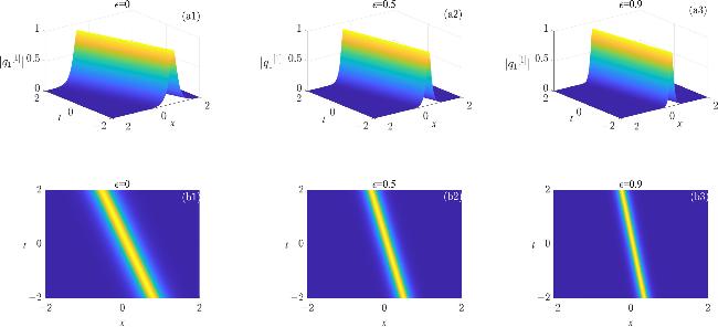
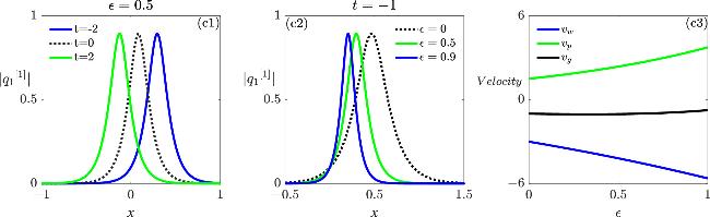
Their images are indicated in figures 2 and 3. From equation (112), we obtain that ${q}_{1}^{[1]}$ and ${q}_{2}^{[1]}$ are essentially the same, with differences only in the amplitude coefficients ${v}_{11}^{* }$ and ${v}_{12}^{* }$. When v11 = 1, v12 = 2 and ${\zeta }_{1}=1+\frac{{\rm{i}}}{2}$, the three-dimensional and the density images of ${q}_{1}^{[1]}$ are shown in figure 2 for the fractional exponent ε = 0, 0.5, 0.9. At ε = 0.5, the wave propagation plot of ${q}_{1}^{[1]}$ along the x-axis at t = −2, 0, 2 is shown in figure 3(c1). We find that ${q}_{1}^{[1]}$ behaves as a left-traveling wave soliton at ε = 0.5. Figure 3(c2) displays the wave propagation plot of ${q}_{1}^{[1]}$ at t = −1 for ε = 0, 0.5, 0.9. It is evident that as ε increases, the displacement of the soliton decreases.
Figure 3. (c1): When ε = 0.5, the wave propagation plot of ${q}_{1}^{[1]}$ along the x-axis at t = −2, 0, 2. (c2): When t = −1, the wave propagation plot of ${q}_{1}^{[1]}$ along the x-axis at ε = 0, 0.5, 0.9. (c3): The wave velocity, phase velocity and group velocity of the fractional one-soliton solution ${q}_{1}^{[1]}$ by choosing ξ1 = 1, ${\eta }_{1}=\frac{1}{2}$.
Moreover, it is known that fractional one-soliton solutions ${q}_{1}^{[1]}$ and ${q}_{2}^{[1]}$ have the same wave velocity vw, phase velocity vp and group velocity vg
From figure 3(c3), we observe that the absolute values of the three velocities increase as ε increases. It is worth noting that the three velocities have a power-law relationship with the amplitude, suggesting that the FCGI equation predicts anomalous dispersion.
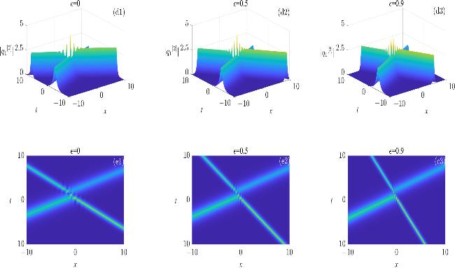
Taking N = 2, ζ1 = ξ1 + iη1 and ζ2 = ξ2 + iη2, the fractional two-soliton solutions of the FCGI equation are derived
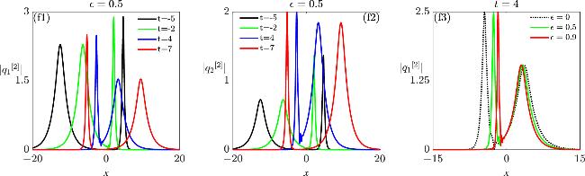
Their images are shown in figures 4 and 5. When ${\zeta }_{1}=\frac{1}{2}+\frac{3}{5}{\rm{i}}$ and ${\zeta }_{2}=\frac{9}{10}+\frac{4}{5}{\rm{i}}$, the three-dimensional images and the density images of ${q}_{1}^{[2]}$ are indicated in figure 4 with the fractional exponent ε = 0, 0.5, 0.9. At t → ±∞, the right-traveling wave with higher energy and the left-traveling wave with lower energy are far apart. After a strong collision, their energies convert between each other while maintaining their original velocities, yet the total energy remains conserved before and after the collision. When ε = 0.5, the wave propagation plot of ${q}_{1}^{[2]}$ and ${q}_{2}^{[2]}$ along the x-axis at t = −5, −2, 4, 7 are shown in figures 5(f1)–(f2). In addition, figure 5(f3) shows the wave propagation plot of ${q}_{1}^{[2]}$ at t = 4 when ε = 0, 0.5, 0.9. It is evident that as the power ε of the fractional derivative increases, the width of the soliton decreases, and the soliton moves increasingly closer.
Figure 5. (f1): When ε = 0.5, the wave propagation plot of ${q}_{1}^{[2]}$ along the x-axis at t = −5, −2, 4, 7. (f2): When ε = 0.5, the wave propagation plot of ${q}_{2}^{[2]}$ along the x-axis at t = −5, −2, 4, 7. (f3): When t = 4, the wave propagation plot of ${q}_{1}^{[2]}$ along the x-axis at ε = 0, 0.5, 0.9.
Next, we examine the long-time asymptotic behavior of the fractional N-soliton solutions in equation (110).
When vk1 = vk2 = 1(1 ≤ k ≤ N), the fractional N-soliton solution ${q}_{1}^{[N]}$ and ${q}_{2}^{[N]}$ of the FCGI equation can be approximated as the sum of N fractional one-soliton solutions as t → ±∞.
Set ζj = ξj + iηj(1 ≤ j ≤ N), where ζj reside in the first quadrant, and define θj = θj,R + iθj,I. Without loss of generality, we suppose vw,N < ⋯ < vw,2 < vw,1 < 0, where ${v}_{w,j}=-{2}^{\epsilon +2}\left({\xi }_{j}^{2}-{\eta }_{j}^{2}\right){\left({\xi }_{j}^{2}+{\eta }_{j}^{2}\right)}^{\epsilon }$ is the velocity of the jth one-soliton solution. When t → −∞, in the reference frame that is moving with a velocity of vw,k(1 ≤ k ≤ N), we have
Hence, it can be concluded that both the amplitude ${h}_{k}=\frac{4{\xi }_{k}{\eta }_{k}}{\left({\xi }_{k}-{\rm{i}}{\eta }_{k}\right)\sqrt{{\varpi }_{k}{f}_{k}}}$ and velocity ${v}_{w,k}=-{2}^{\epsilon +2}\left({\xi }_{k}^{2}-{\eta }_{k}^{2}\right){\left({\xi }_{k}^{2}+{\eta }_{k}^{2}\right)}^{\epsilon }$ of soliton-k are preserved after the interaction. However, their positions and phases undergo shifts.
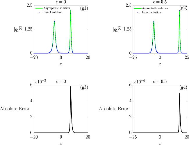
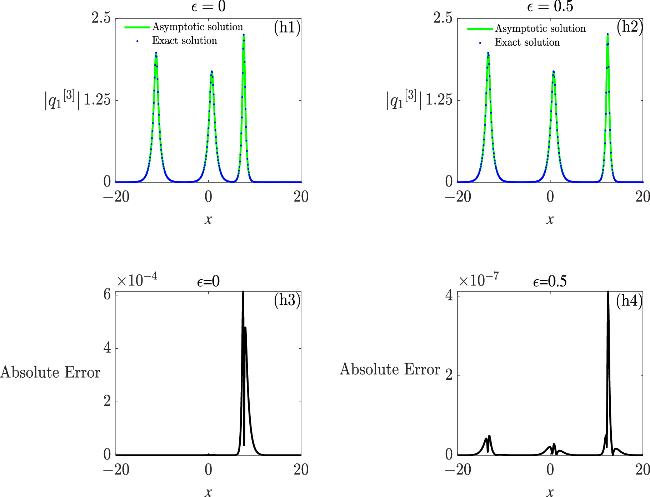
According to theorem 1, we present the comparison plots between the exact solutions and the asymptotic solutions of the fractional two-soliton and three-soliton solutions at t = −10, along with the absolute error plots between the exact and asymptotic solutions in figures 6 and 7.
Figure 6. (g1)–(g2): The comparison plot of the exact and asymptotic expressions of the two-soliton solution at t = −10 for ε = 0, 0.5. (g3)–(g4): When ε = 0, the absolute error ($| {q}_{1,-}^{[2]}-{q}_{1}^{[2]}| $) plot between the exact and asymptotic expressions of the two-soliton solution at t = −10.
Figure 7. (h1)–(h2): The comparison plot of the exact and asymptotic expressions of the three-soliton solution at t = −10 for ε = 0, 0.5. (h3)–(h4): When ε = 0, 0.5, the absolute error ($| {q}_{1,-}^{[3]}-{q}_{1}^{[3]}| $) plot between the exact and asymptotic expressions of the three-soliton solution at t = −10.
6. Conclusions
In this paper, by considering the 3 × 3 AKNS spectral problem and the Riesz fractional derivative, the integrable FCGI equation is constructed. Then, based on the completeness relation of the squared eigenfunctions, the explicit form of the FCGI equation is derived. Subsequently, in the reflectionless case, the fractional N-soliton solutions of the FCGI equation are given by means of the RH method. In particular, by analyzing the dynamical behavior of the soliton solutions, we know that as the power ε of the Riesz fractional derivative increases, the amplitudes of the soliton solutions remain unchanged, while their wave widths decrease. Moreover, the absolute values of wave velocity, phase velocity, and group velocity are positively correlated with ε and maintain a power-law relationship with the amplitude, indicating that the FCGI equation can predict anomalous dispersion phenomena. Finally, we analyze the long-time asymptotic behavior of the fractional N-soliton solutions as t → ±∞. It is worth noting that the asymptotic analysis method adopted in this work has been improved and successfully applied to the study of higher-order soliton solutions in integrable systems [42–44]. This lays a solid foundation for further exploration of the RH problems with higher-order poles in fractional integrable equations and for the analysis of the long-time asymptotic behavior of fractional higher-order soliton solutions.
WangB H, WangY Y, DaiC Q, ChenY X2020 Dynamical characteristic of analytical fractional solitons for the space-time fractional Fokas–Lenells equation Alexandria Engin. J.59 4699 4707
GoufoE F D2016 Application of the Caputo–Fabrizio fractional derivative without singular kernel to Korteweg–de Vries–Burgers equation Math. Model. Anal.21 188 198
RavichandranC, LogeswariK, JaradF2019 New results on existence in the framework of Atangana–Baleanu derivative for fractional integro-differential equations Chaos Soliton Fract.125 194 200
DaiC Q, FanY, ZhangN2019 Re-observation on localized waves constructed by variable separation solutions of (1+1)-dimensional coupled integrable dispersionless equations via the projective Riccati equation method Appl. Math. Lett.96 20 26
KumarD, SinghJ, BaleanuD, Sushila2018 Analysis of regularized long-wave equation associated with a new fractional operator with Mittag–Leffler type kernel Physica A492 155 167
DaiC Q, FanY, WangY Y2019 Three-dimensional optical solitons formed by the balance between different-order nonlinearities and high-order dispersion in parity-time symmetric potentials Nonlinear Dyn.98 489 499
ChenS J, LinJ N, WangY Y2019 Soliton solutions and their stabilities of three (2+1)-dimensional PT-symmetric nonlinear Schrödinger equations with higher-order diffraction and nonlinearities Optik194 162753
FengQ, MengF2020 Mathematical analysis of a fractional differential model of HBV infection with antibody immune response Chaos Solitons Fract.136 109787
MioK, OginoT, MinamiK, TakedaS1976 Modulational instability and envelope-solitons for nonlinear Alfvén waves propagating along the magnetic field in plasmas J. Phys. Soc. Jpn.41 667 673
GerdjikovV S, IvanovM I1982 The quadratic bundle of general form and the nonlinear evolution equations JINR-E--2-82-545 Joint Inst. for Nuclear Research, Dubna (USSR), Lab. of Theoretical Physics
30
GerdzhikovV S, IvanovM I2012 A quadratic pencil of general type and nonlinear evolution equations. I. expansions in ‘squares' of solutions-generalized Fourier transforms Rev. Adm.47 22 37
31
WadatiM, SogoK1983 Gauge transformations in soliton theory J. Phys. Soc. Japan52 394 398
PeiL M, LiB2011 The Darboux transformation of the Gerdjikov-Ivanov equation from non-zero seed International Conference on Consumer Electronics, Communications and Networks (CECNet), IEEE 5320 5323
34
ZhaoP, FanE G2020 Finite gap integration of the derivative nonlinear Schrödinger equation: a Riemann–Hilbert method Physica D402 132213
YangJ K2010Nonlinear Waves in Integrable and Nonintegrable Systems Philadelphia, PA SIAM
42
LiM, ZhangX F, XuT, LiL L2020 Asymptotic analysis and soliton interactions of the multi-pole solutions in the Hirota equation J. Phys. Soc. Jpn.89 054004
LiY, LiM, XuT, HuangY H, XuC X2025 N-soliton solutions and asymptotic analysis for the massive Thirring model in the laboratory coordinates via the Riemann–Hilbert approach Commun. Theor. Phys.77 065003


