


1. Introduction
A biased noise model is developed to generate asymmetric noise vectors, which serve as the input dataset for the neural network.
A neural network decoding algorithm based on the belief propagation framework is proposed. By utilizing a customized multi-objective loss function, the algorithm performs back error correction and mitigates the issue of quantum error degeneracy during quantum information transmission. The decoding threshold on surface codes reaches 20%.
Several convolutional optimization schemes are discussed, which accelerate the convergence speed of the proposed algorithm.
Numerical results show that for bias-tailored quantum codes, NBP + CNN + BIAS performs better than BP + OSD. Our proposed NBP + CNN + BIAS decoder achieves an order of magnitude improvement in their error suppression relative to higher-order BP + OSD.
2. Preliminaries
2.1. Calderbank-shor-steane codes
2.2. Bias-tailored XZZX codes
3. Neural belief propagation decoder
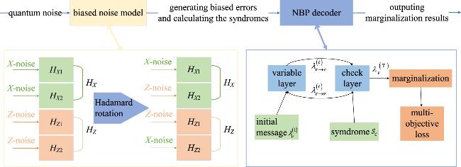
Figure 1. The structure of NBP + BIAS decoder. The decoder mainly consists of a biased noise model and a neural belief propagation (NBP) decoder using a multi-objective loss function. |
The quantum channel generates simulated asymmetric noise, which is received by the quantum biased noise model. This model produces the rotated asymmetric noise errors X and Z required by the decoder and applies them to the HZ and HX matrices (see equations (
The input information to NBP consists of equation (
The marginalized probability λv is used to infer errors through the equation
Verify whether the results $\widehat{{\boldsymbol{e}}}$ satisfy $({\boldsymbol{e}}+\widehat{{\boldsymbol{e}}})\cdot {{\boldsymbol{H}}}_{i}^{\perp }=0$. If the condition is not met, logical errors have occurred.
Additionally, the convolution operation mentioned in section
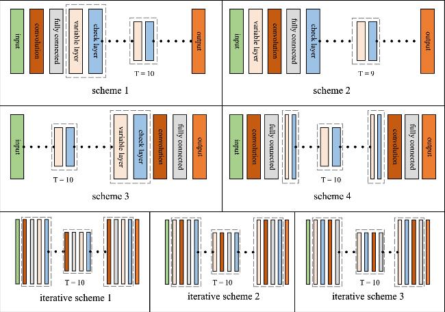
Figure 2. Convolutional optimization schemes. The symbol ‘⋯' represents a repeating structure and ‘T' is the number of repetitions. |
3.1. Biased noise model
Biased noise model
| Input: CSS parity check matrices HX and HZ; code length N; column length N1 of HX1; Pauli error rates εX, εY, εZ |
| Output: errors eX and eZ |
| 1: eX = 0, eZ = 0 |
| 2: pX = 0, pZ = 0 |
| 3: Hadamard rotation |
| 4: for i = 1 to N1 |
| 5: pX[i] = εX + εY |
| 6: pZ[i] = εZ + εY |
| 7: end for |
| 8: for i = N1 + 1 to N |
| 9: pX[i] = εZ + εY |
| 10: pZ[i] = εX + εY |
| 11: end for |
| 12: generate random errors |
| 13: for i = 1 to N |
| 14: ξ = random(0, 1) |
| 15: if ξ < pX[i] |
| 16: eX[i] = 1, eZ[i] = 0 |
| 17: else if pX[i] < ξ < pX[i] + pZ[i] |
| 18: eX[i] = 0, eZ[i] = 1 |
| 19: else if pX[i] + pZ[i] < ξ < pX[i] + pZ[i] + εY |
| 20: eX[i] = 1, eZ[i] = 1 |
| 21: end if |
| 22: end for |
| 23: return eX, eZ |
3.2. Neural belief propagation
At position (0,0), the matrix entry is 1. We duplicate the row [1,1,0], set the 0th element to 0, yielding [0,1,0], and store it as the 0th column of w.
At position (0,1), the entry is 1. We duplicate the row [1,1,0], set the 1st element to 0, yielding [1,0,0], and store it as the 1st column of w.
At position (0,2), the entry is 0. This entry is skipped.
At position (1,0), the entry is 0. This entry is skipped.
At position (1,1), the entry is 1. We duplicate the row [0,1,1], set the 1st element to 0, yielding [0,0,1], and store it as the 2nd column of w.
At position (1,2), the entry is 1. We duplicate the row [0,1,1], set the 2nd element to 0, yielding [0,1,0], and store it as the 3rd column of w.
3.3. Multi-objective loss function
4. Convolutional optimization schemes
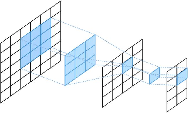
Figure 3. Structure of convolutional step. |
5. Numerical results
5.1. Experimental environment and parameter definitions
Table 1. Experimental setup. |
| Parameter | value |
|---|---|
| learning rate | 0.0001 |
| number of hidden layers | 20 |
| number of BP iterations | 10 |
| total number of batches | 40000 |
| number of batches per epoch | 1000 |
| physical error rate ε | 0.01 ∼ 0.26 |
| batch size for each physical error rate | 30 |
| error bias Bi | {0.5, 5, 10, 30, 50} |
| convolutional layer parameters | {3 × 3, 16;1 × 1, 8} |
| batch size for validation set | 50 |
Table 2. Statistics of classical error rate and logical error rate for bias-tailored quantum code [[12, 2, 3]] under different hyperparameters a. The physical error rate ε is 0.06. |
| The value of a | classic error rate | logical error rate |
|---|---|---|
| 0.1 | 0.020292 | 0.016583 |
| 0.2 | 0.018125 | 0.014854 |
| 0.3 | 0.015646 | 0.011083 |
| 0.4 | 0.015875 | 0.012583 |
| 0.5 | 0.015854 | 0.013354 |
| 0.8 | 0.018937 | 0.015229 |
| 1.0 | 0.020958 | 0.020667 |
5.2. Decoder performance optimization
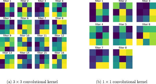
Figure 4. Visualization of the spatial structure of convolutional kernels. All the data results are obtained with a physical error rate of ε = 0.1. |
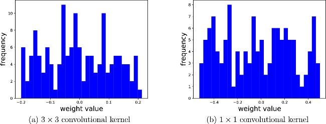
Figure 5. Histogram of the weight distribution of convolutional kernels. All the data results are obtained with a physical error rate of ε = 0.1. |
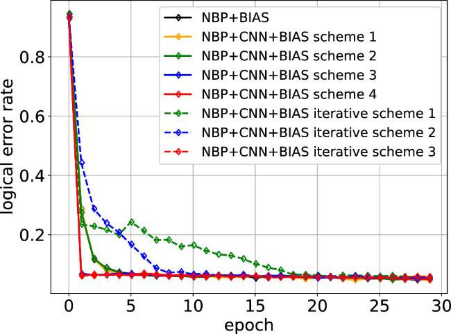
Figure 6. Comparison of convergence speeds for different convolutional schemes on [[58,16,3]]. All the data results are obtained with a physical error rate of ε = 0.1. |
Table 3. Observed thresholds for numerical simulations of the decoders applied to Surface codes (d = 3, 5, 7). ‘*' represents the case of circuit-level noise. |
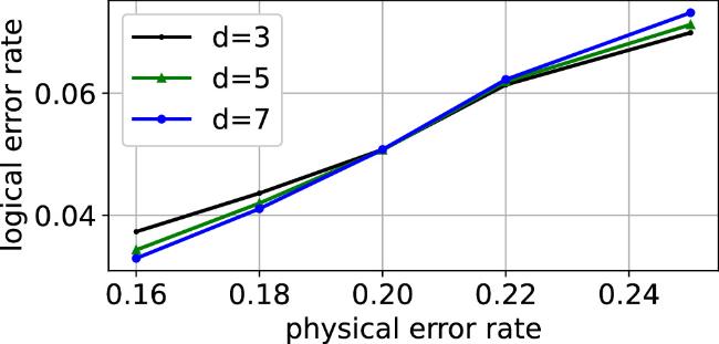
Figure 7. Decoding Surface codes with NBP + CNN + BIAS. |
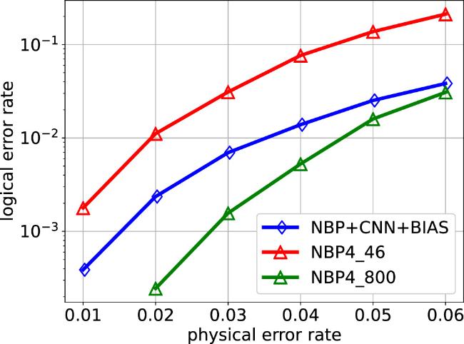
Figure 8. Performance comparison of two decoders on [[46,2,9]]. |
5.3. Decoding performance on biased noise channels
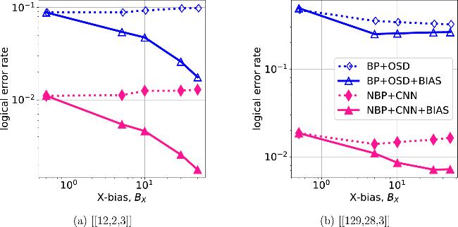
Figure 9. Standard CSS quantum codes versus bias-tailored XZZX quantum codes. All legends with the suffix ‘BIAS' represent the decoding of the bias-tailored codes using the biased noise model. All the data results are obtained with a physical error rate of ε = 0.06. The OSD orders of [[12,2,3]] and [[129,28,3]] are 7 and 30, respectively. |
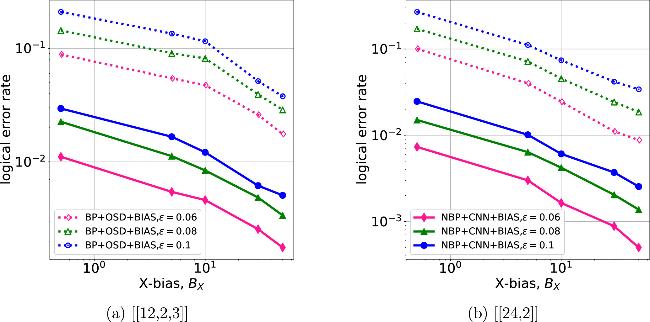
Figure 10. Simulation curves of bias-tailored quantum codes [[12,2,3]] and [[24,2]] under different physical error rates. The OSD orders of [[12,2,3]] and [[24,2]] are 7 and 13, respectively. |