

1. Introduction
Optical interferometers are among the most precise measurement instruments and have been widely employed in diverse fields, such as gravitational wave detection [1, 2], quantum imaging [3, 4], quantum ranging [5] and quantum lithography [6]. The ultimate sensitivity for estimating an unknown phase in an interferometer is typically determined by the state of input light. When classical light is used, the sensitivity is bounded by the shot noise limit $1/\sqrt{N}$, where N is the average photon number [7–9]. In contrast, non-classical states of light can surpass this limit. Among them, NOON states are particularly renowned for their ability to achieve Heisenberg-limited sensitivity, which scales as 1/N [7–9]. More recently, entangled coherent states (ECSs) have emerged as promising candidates for phase estimation as they not only surpass the Heisenberg limit for small N but also exhibit greater robustness to photon loss compared to NOON states [10–17].
To fully leverage the advantages of non-classical light, an effective and sensitive measurement is required [18–21]. In practical implementations, photon-number-resolving detectors constitute a crucial class of measurement schemes, such as parity and photon count [22–31]. These detectors are experimentally favorable, as they can be implemented without the need for a shared reference beam. However, previous studies on phase estimation with ECSs have been conducted under the assumption that a common reference beam is already established [10–14, 17]. As a result, the findings reported in these works are generally not applicable to measurement schemes involving photon-number-resolving detectors. This naturally raises the question: how do ECSs perform in phase estimation when the reference beam is absent? More specifically, what is the ultimate phase sensitivity achievable for ECSs when using photon-number resolving detectors?
In this paper, we address this issue b re-examining the metrological performance of ECSs in a lossy interferometer. Using the quantum Fisher information (QFI) framework [18–21], we evaluate the ultimate sensitivity for both scenarios with and without a reference beam. Although it is commonly acknowledged that these two scenarios yield equivalent sensitivities under ideal lossless conditions for the two-phase-shifting configuration [15, 32], our results show that significant differences arise in the presence of photon loss. Specifically, not only does the equivalence break down, but also the disadvantage of ECSs relative to NOON states observed in the presence of reference beam also disappears when the reference beam is omitted.
This paper is organized as follows. In section 2 , we introduce the two-mode optical interferometer and review the fundamentals of quantum estimation theory. Section 3 provides a comprehensive comparison of phase sensitivities for ECSs with and without a reference beam. Finally, we conclude in section 4 .
2. Phase estimation with a two-mode optical interferometer
A two-mode optical interferometer enables precise measurement of the phase difference between the two paths (see figure 1). A typical interferometer comprises two balanced beam splitters (BSs) ${B}_{i}\left(i=1,2\right)$ and a phase shifter Uφ with an unknown phase parameter φ [33]. As photons propagate between the BSs, the phase of interest is accumulated. The overall interferometric evolution can be described by the composite operator K = B2UφB1. If ρin denotes the state entering the interferometer, then the output state is given by ρout = KρinK†. Measurements performed at the output ports provide information to estimate the unknown phase parameter.
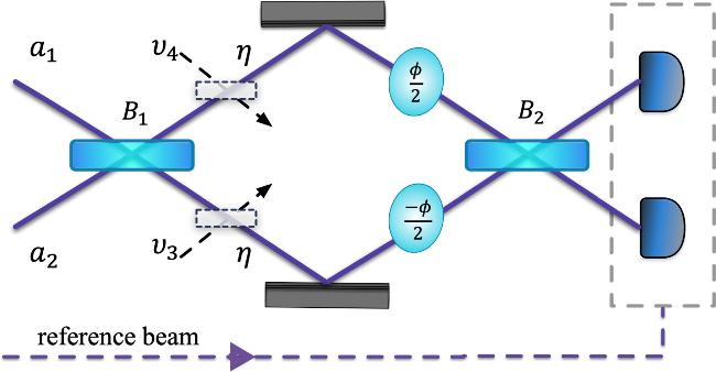
Figure 1. Schematic of a two-mode lossy optical interferometer. |
For convenience, we refer to the probe state as the state prior to the phase-shifting operation, i.e., $\rho ={B}_{1}{\rho }_{{\rm{in}}}{B}_{1}^{\dagger }$. Under the action of the phase shifter Uφ, the state evolves into the phase-encoded state ${\rho }_{\phi }={U}_{\phi }\rho {U}_{\phi }^{\dagger }$. According to quantum estimation theory, the quantum Cramér–Rao theorem sets a fundamental lower bound on the phase uncertainty $\delta \hat{\phi }$ for any locally unbiased estimator $\hat{\phi }$ [18, 34, 35]:
$\begin{eqnarray}\delta \hat{\phi }\geqslant {(mF)}^{-1/2},\end{eqnarray}$
where m is the number of repetitions of an experiment, and F is the QFI defined as $F={\rm{Tr}}\left({\rho }_{\phi }{L}^{2}\right)$. Here, L is the symmetric logarithmic derivative operator implicitly defined by ${\rm{d}}{\rho }_{\phi }/{\rm{d}}\phi =\left({\rho }_{\phi }L+L{\rho }_{\phi }\right)/2$. This bound is asymptotically achievable and serves as a benchmark for assessing the performance of phase estimation protocols. In interferometric phase estimation, the QFI depends solely on the phase-encoded state ρφ, regardless of the second BS B2 due to the φ-independent unitary invariance of the QFI [36].We consider two commonly used forms of phase-shifting unitary operators. The first is the two-arm phase shift
$\begin{eqnarray}{U}_{\phi }^{T}={\rm{\exp }}\left[-{\rm{i}}\phi \left({a}_{1}^{\dagger }{a}_{1}-{a}_{2}^{\dagger }{a}_{2}\right)/2\right],\end{eqnarray}$
which introduces a different phase shift by applying phase shifts of φ/2 and −φ/2 to the two interferometer paths, respectively. Here, ai and ${a}_{i}^{\dagger }$ denote the annihilation and creation operators for the ith mode (i = 1, 2), respectively. The second is the single-arm phase shift ${U}_{\phi }^{S}={{\rm{e}}}^{-{\rm{i}}\phi {a}_{1}^{\dagger }{a}_{1}}$, which applies the full phase shift φ to a single path. Notably, these two phase-shifting operators are metrologically equivalent in the absence of reference beam [15, 32]. This equivalence stems from the fact that ${U}_{\phi }^{S}$ differs from ${U}_{\phi }^{T}$ only up to a sum phase shift ${U}_{\phi }^{\&}={\rm{\exp }}[-{\rm{i}}\phi ({a}_{1}^{\dagger }{a}_{1}+{a}_{2}^{\dagger }{a}_{2})/2]$, which is experimentally immeasurable without introducing an external phase reference.More precisely, in reference-free scenarios, the probe state must be phase-averaged as [32, 37]
$\begin{eqnarray}\varrho ={\int }_{-\pi }^{\pi }\frac{{\rm{d}}\theta }{2\pi }{U}_{\theta }^{{a}_{1}}{U}_{\theta }^{{a}_{2}}\rho {U}_{\theta }^{{a}_{1}\dagger }{U}_{\theta }^{{a}_{2}\dagger },\end{eqnarray}$
with ${U}_{\theta }^{x}=\exp (-{\rm{i}}\theta {x}^{\dagger }x)$. The resulting phase-averaged state is a statistical ensemble of states with fixed photon numbers, resulting in the loss of coherence between different photon-number subspaces. Consequently, such states are insensitive to ${U}_{\phi }^{\&}$, rendering ${U}_{\phi }^{S}$ and ${U}_{\phi }^{T}$ operationally indistinguishable in phase estimation. In other words, for a given probe state, the ultimate phase sensitivity is independent of the specific form of the phase-shifting operation in the absence of a reference beam. However, once an external reference beam is established, the sum phase becomes physically meaningful, and the two configurations ${U}_{\phi }^{S}$ and ${U}_{\phi }^{T}$ become distinguishable, leading to potentially different metrological performances.In this work, we focus on the ${U}_{\phi }^{T}$ configuration for the following reasons: (1) in the ideal lossless case, the QFI under ${U}_{\phi }^{T}$ is identical irrespective of the presence or absence of a reference beam. However, whether this equivalence persists under photon loss remains an open question, which is one of the issues we aim to address. (2) The ${U}_{\phi }^{S}$ configuration has been extensively studied in previous studies [11–14, 16], and the methodology developed here for ${U}_{\phi }^{T}$ can be straightforwardly adapted to analyze ${U}_{\phi }^{S}$ as well.
3. Phase sensitivity of lossy interferometry with ECSs
In this section, we investigate the phase sensitivity of a lossy interferometer using ECSs as the probe state. Photon loss is modeled by inserting a virtual BS with transmittance η into each interferometer path, denoted by the operator Vη [12, 38, 39]. For simplicity, we assume equal photon loss in both interferometer paths. ECSs can be generated by mixing coherent and coherent superposition states of light on a BS [10], or alternatively generated by mixing coherent and squeezed vacuum states of light on a BS [40]. The resulting ECS is given by
$\begin{eqnarray}\left|{\rm{ECS}}\right\rangle ={ \mathcal N }\left(| \alpha \rangle | 0\rangle +| 0\rangle | \alpha \rangle \right),\end{eqnarray}$
with normalization coefficient ${ \mathcal N }=1/\sqrt{2(1+{{\rm{e}}}^{-{\left|\alpha \right|}^{2}})}$. This state can be expanded as a superposition of NOON states $\begin{eqnarray}\left|{\rm{ECS}}\right\rangle =\sqrt{2}{ \mathcal N }\displaystyle \sum _{n=0}^{\infty }| {c}_{n}{| }^{2}| n::0\rangle ,\end{eqnarray}$
where ${c}_{n}={{\rm{e}}}^{-| \alpha {| }^{2}/2}{\alpha }^{n}/\sqrt{n!}$, and $| n\,::\,0\rangle \equiv (| n\rangle | 0\rangle +| 0\rangle | n\rangle )/\sqrt{2}$ denotes a NOON state with fixed photon number n. The average photon number of the ECS is $\overline{N}=2{{ \mathcal N }}^{2}| \alpha {| }^{2}$. In the limit of large $\left|\alpha \right|$, this approaches $\overline{N}\sim | \alpha {| }^{2}$ since ${ \mathcal N }\sim 1/\sqrt{2}$. In what follows, we compute the QFI for ECS-based phase estimation within two distinct scenarios: with and without a reference beam.3.1. Phase sensitivity without a reference beam
We first consider the scenario in which no reference beam is available. In this case, the phase-averaging operation defined in equation (3 ) must be applied. As a result, the ECS probe state given in equation (4 ) becomes a mixed state, which can be expressed as a direct sum of weighted NOON states [15, 36]7 ) can be expressed in the compact form
$\begin{eqnarray}{\varrho }_{{\rm{ECS}}}=2{{ \mathcal N }}^{2}\displaystyle \underset{n=0}{\overset{\infty }{\oplus }}{\left|{c}_{n}\right|}^{2}\left|n::0\right\rangle \left\langle n::0\right|.\end{eqnarray}$
According to the additivity property of the QFI, the QFI for this phase-averaged ECS can be directly calculated as $\begin{eqnarray}{F}_{\varrho }=2{{ \mathcal N }}^{2}\displaystyle \sum _{n=0}^{\infty }{\left|{c}_{n}\right|}^{2}{F}_{{\rm{noon}}},\end{eqnarray}$
where Fnoon = n2ηn is the QFI for small NOON states used as probe states in a lossy interferometer [13, 31]. Equation ( $\begin{eqnarray}{F}_{\varrho }=2{{ \mathcal N }}^{2}{{\rm{e}}}^{-{\left|\alpha \right|}^{2}\left(1-\eta \right)}\left({\left|\alpha \right|}^{4}{\eta }^{2}+{\left|\alpha \right|}^{2}\eta \right).\end{eqnarray}$
In this expression, the first term inside the parentheses represents the Heisenberg-scaling contribution, while the second term corresponds to shot-noise scaling. This result is valid for both the single-phase and two-phase configurations (${U}_{\phi }^{S}$ and ${U}_{\phi }^{T}$), as justified in preceding section. In the ideal lossless case (η = 1), the QFI simplifies to [15] $\begin{eqnarray}{F}_{\varrho }=2{{ \mathcal N }}^{2}\left(| \alpha {| }^{4}+| \alpha {| }^{2}\right).\end{eqnarray}$
Expressing in terms of mean photon number, we have ${F}_{\varrho }\geqslant {\overline{N}}^{2}+\overline{N}$, thereby surpassing the conventional Heisenberg limit. This result demonstrates that ECSs offer superior phase sensitivity compared to NOON states with the same average photon number.3.2. Phase sensitivity with a reference beam
For comparison, we now consider the scenario in which a common reference beam is available, and the probe state is the pure ECS defined in equation (4 ). In this case, the phase-shifting operation is implemented using the operator ${U}_{\phi }^{T}$. Unlike the reference-free scenario, calculating the QFI in the presence of a reference beam is more intricate. Below, we summarize the key steps in the calculation, while full derivations are provided in the Appendix .
Owing to the commutation relationship between photon loss and phase shifting [38, 39], the order of these operations can be interchanged without affecting the final measurement results. Thus, we assume that the ECS in equation (4 ) first undergoes photon loss, followed by the phase accumulation process. Under such a loss, the ECS evolves into a mixed state as 12 ), the expansion coefficients are defined as
$\begin{eqnarray}\begin{array}{rcl}{\sigma }_{{\rm{ECS}}} & = & {{\rm{Tr}}}_{34}\left[{V}_{13}{V}_{24}\left(| {\rm{ECS}}{\rangle }_{12}{\langle {\rm{ECS}}| \displaystyle \otimes | 00\rangle }_{34}\langle 00| \right){V}_{24}^{\dagger }{V}_{13}^{\dagger }\right]\\ & = & {{ \mathcal N }}^{2}\left(| \alpha \sqrt{\eta },0\rangle \langle \alpha \sqrt{\eta },0| +| 0,\alpha \sqrt{\eta }\rangle \langle 0,\alpha \sqrt{\eta }| \right.\\ & & +{{\rm{e}}}^{-\left(1-\eta \right){\left|\alpha \right|}^{2}}| \alpha \sqrt{\eta },0\rangle \langle 0,\alpha \sqrt{\eta }| \\ & & \left.+{{\rm{e}}}^{-\left(1-\eta \right){\left|\alpha \right|}^{2}}| 0,\alpha \sqrt{\eta }\rangle \langle \alpha \sqrt{\eta },0| \right),\end{array}\end{eqnarray}$
where $| 0{\rangle }_{k}\left(k=3,4\right)$ denotes the vacuum states of the environmental modes corresponding to paths 1 and 2, respectively. Here the virtual beam splitters are defined as V13 and V24 define ${V}_{13}=\exp [\arccos \sqrt{\eta }({a}_{1}^{\dagger }{\upsilon }_{3}-{a}_{1}{\upsilon }_{3}^{\dagger })]$, and V24 is defined analogously by substituting modes 1 and 3 with modes 2 and 4. Let $| {{\Psi }}_{1}\rangle =| \alpha \sqrt{\eta },0\rangle $ and $| {{\Psi }}_{2}\rangle =| 0,\alpha \sqrt{\eta }\rangle $. These states are non-orthogonal, with overlap $p\equiv \langle {{\Psi }}_{1}| {{\Psi }}_{2}\rangle ={{\rm{e}}}^{-\eta {\left|\alpha \right|}^{2}}$. Employing the Gram–Schmidt orthogonalization and performing spectral decomposition [14, 16], the state σECS can be diagonalized as $\begin{eqnarray}{\sigma }_{{\rm{ECS}}}={\gamma }_{+}| {\gamma }_{+}\rangle \langle {\gamma }_{+}| +{\gamma }_{-}| {\gamma }_{-}\rangle \langle {\gamma }_{-}| ,\end{eqnarray}$
where the eigenstates take the form $\begin{eqnarray}\left|{\gamma }_{\pm }\right\rangle ={{ \mathcal C }}_{\pm }\left|{{\Psi }}_{1}\right\rangle +{{ \mathcal D }}_{\mp }\left|{{\Psi }}_{2}\right\rangle ,\end{eqnarray}$
and the corresponding eigenvalues are given by $\begin{eqnarray}{\gamma }_{\pm }=\frac{1}{2}\left(1\pm \sqrt{1-\det {\sigma }_{{\rm{ECS}}}}\right).\end{eqnarray}$
In equation ( $\begin{eqnarray}{{ \mathcal C }}_{\pm }=\pm {\zeta }_{\pm }-p{{ \mathcal D }}_{\mp },\ {{ \mathcal D }}_{\mp }=\frac{{\zeta }_{\mp }}{\sqrt{1-{p}^{2}}},\end{eqnarray}$
with ${\zeta }_{\pm }=\sqrt{\frac{\sqrt{1-4\det {\sigma }_{{\rm{ECS}}}}\pm \langle {\sigma }_{3}\rangle }{2\sqrt{1-4\det {\sigma }_{{\rm{ECS}}}}}},$ $\det {\sigma }_{{\rm{ECS}}}={{ \mathcal N }}^{4}(1-{p}^{2})(1-{p}_{\perp }^{2})$, $\langle {\sigma }_{3}\rangle =1-2{{ \mathcal N }}^{2}(1-{p}^{2})$ and ${p}_{\perp }={{\rm{e}}}^{-(1-\eta ){\left|\alpha \right|}^{2}}$.The QFI for the mixed state σECS is then obtained by 2 ). To compute Δ2G± and G+−, we use the following expectation values 15 ) yields the full expression for Fσ. Although this expression is algebraically cumbersome, it simplifies, in the limit p → 0 (i.e., η∣α∣2 ≫ 1), to 9 ), i.e., Fϱ = Fσ, thereby confirming that, for the two-phase-shifting operation ${U}_{\phi }^{T}$, the metrological performance remains invariant regardless of the presence or absence of a reference beam. This result is consistent with the commonly acknowledged conclusion reported in [15, 32], namely that the phase shifter ${U}_{\phi }^{T}$ exhibits metrological equivalence between scenarios with and without a reference beam for phase estimation protocols employing pure probe states. However, as we demonstrate below, in the presence of photon loss, ECSs with and without a reference beam exhibit distinct metrological behavior, indicating that this equivalence does not extend to lossy conditions.
$\begin{eqnarray}{F}_{\sigma }=4\left({\gamma }_{+}{{\rm{\Delta }}}^{2}{G}_{+}+{\gamma }_{-}{{\rm{\Delta }}}^{2}{G}_{-}-4{\gamma }_{+}{\gamma }_{-}{\left|{G}_{+-}\right|}^{2}\right),\quad \end{eqnarray}$
where $\begin{eqnarray}{{\rm{\Delta }}}^{2}{G}_{\pm }=\left\langle {\gamma }_{\pm }\right|{G}^{2}\left|{\gamma }_{\pm }\right\rangle -\left\langle {\gamma }_{\pm }\right|G{\left|{\gamma }_{\pm }\right\rangle }^{2},\end{eqnarray}$
$\begin{eqnarray}{G}_{+-}=\left\langle {\gamma }_{+}\right|G\left|{\gamma }_{-}\right\rangle ,\end{eqnarray}$
and $G=({a}_{1}^{\dagger }{a}_{1}-{a}_{2}^{\dagger }{a}_{2})/2$ is the generator of ${U}_{\phi }^{T}$ defined in equation ( $\begin{eqnarray}\left\langle {{\Psi }}_{1}\right|G\left|{{\Psi }}_{1}\right\rangle =\frac{1}{2}{\left|\alpha \right|}^{2}\eta ,\quad \left\langle {{\Psi }}_{2}\right|G\left|{{\Psi }}_{2}\right\rangle =\frac{1}{2}{\left|\alpha \right|}^{2}\eta ,\end{eqnarray}$
$\begin{eqnarray}\left\langle {{\Psi }}_{i}\right|{G}^{2}\left|{{\Psi }}_{i}\right\rangle =\frac{1}{4}\left({\left|\alpha \right|}^{2}\eta +{\left|\alpha \right|}^{4}{\eta }^{2}\right),\quad {\rm{for}}\,i=1,2,\end{eqnarray}$
$\begin{eqnarray}\left\langle {{\Psi }}_{1}\right|{G}^{2}\left|{{\Psi }}_{2}\right\rangle =\left\langle {{\Psi }}_{2}\right|{G}^{2}\left|{{\Psi }}_{1}\right\rangle =0.\end{eqnarray}$
Substituting these into equation ( $\begin{eqnarray}{F}_{\sigma }=2{{ \mathcal N }}^{2}\left({{\rm{e}}}^{-2{\left|\alpha \right|}^{2}\left(1-\eta \right)}{\left|\alpha \right|}^{4}{\eta }^{2}+{\left|\alpha \right|}^{2}\eta \right).\end{eqnarray}$
In the ideal lossless case (η = 1), this expression reduces to equation (3.3. Further comparison
To thoroughly assess metrological performance under photon loss, we compare three quantum strategies: (i) ECSs without a reference beam, (ii) ECSs with a reference beam, and (iii) NOON states, whose QFI is given by FNOON = ηNN2 [13, 31], For a fair comparison, we set the same mean photon number $\overline{N}=N$ for both ECSs and NOON states.
Let us first compare the strategies of NOON states and ECSs with a reference beam. As shown in figure 2, the two critical crossing points N1 and N2 exist, defined by the condition FNOON = Fσ. Although their analytical expressions are cumbersome, these crossing points demarcate distinct performance regimes. In the regime N < N1, ECSs with a reference beam outperforms NOON states. However, in the intermediate range N1 < N < N2, this trend reverses with NOON states exhibiting superior performance against ECSs. As N increases further, the QFI of NOON states diverges, whereas the QFI of ECSs with a reference beam asymptotically approaches the shot-noise limit ($\delta \phi \sim 1/\sqrt{\eta N}$). This phenomenon illustrates that although the use of a reference beam enables ECSs to achieve superior sensitivity compared to NOON states at low N, this advantage diminishes at intermediate N. A similar trend has been reported for the single-phase configuration ${U}_{\phi }^{S}$ [13]. Interestingly, ECSs without a reference beam combines the advantages of both strategies: for N < N1, they perform similarly to ECSs with a reference beam, while for N > N1, they resemble NOON states. Consequently, although phase sensitivity deteriorates with increasing loss, omitting the reference beam can be advantageous in ECS-based phase estimation, offering improved performance across a border range of photon numbers.
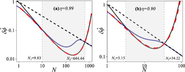


Figure 2. Log-log plot of phase sensitivity as a function of the mean photon number N (with $\overline{N}=N$ for ECSs) for (a) η = 0.99 and (b) η = 0.9. The blue solid line and red dashed line represent ECSs with and without a reference beam, respectively. The black solid line corresponds to the NOON states, and the gray dashed line marks the shot-noise limit $1/\sqrt{\eta N}$ as a benchmark. |
These behaviors are quantitatively supported by equations (8 ) and (21 ). In the low intensity regime, where ${\left|\alpha \right|}^{2}\left(1-\eta \right)\ll 1$, we have ${{\rm{e}}}^{-2{\left|\alpha \right|}^{2}\left(1-\eta \right)}\sim 1$, which leads to 21 ) (which corresponds to the Heisenberg-limit scaling) vanishes due to ${{\rm{e}}}^{-2{\left|\alpha \right|}^{2}\left(1-\eta \right)}\to 0$. This leaves only the second term, which scales as shot noise limit: ${F}_{\sigma }\sim \eta \overline{N}$. By contrast, for ECSs without a reference beam, the behavior resembles that of NOON states in this regime. Recalling that $\overline{N}={\left|\alpha \right|}^{2}$, the QFI from equation (8 ) becomes
$\begin{eqnarray}{F}_{\varrho }={F}_{\sigma }\approx 2{{ \mathcal N }}^{2}\left({\left|\alpha \right|}^{4}{\eta }^{2}+{\left|\alpha \right|}^{2}\eta \right).\end{eqnarray}$
This explains why, in figure 2, the QFIs of both ECS strategies nearly coincide in the low-photon-number regime. In the high intensity regime $\overline{N}\sim {\left|\alpha \right|}^{2}\gg 1$, however, the behavior diverges. For ECSs with a reference beam, the first term in equation ( $\begin{eqnarray}{F}_{\varrho }={{\rm{e}}}^{\left(\overline{N}+2\right)\left(\eta -1\right)}{\overline{N}}^{2}+{{\rm{e}}}^{\overline{N}\left(\eta -1\right)}\overline{N}\eta \approx {{\rm{e}}}^{\overline{N}\left(\eta -1\right)}{\overline{N}}^{2}.\end{eqnarray}$
This scaling is consistent with that of NOON states, for which $\begin{eqnarray}{F}_{{\rm{NOON}}}={\eta }^{N}{N}^{2}\approx {{\rm{e}}}^{N\left(\eta -1\right)}{N}^{2},\end{eqnarray}$
where we have used the approximation $\mathrm{ln}\,\eta \sim \eta -1$ in the limit η → 1.4. Conclusion
In this work, we systematically analyzed the phase estimation performance of a lossy optical interferometer using ECSs as probe states, considering scenarios both with and without a reference beam. Using the QFI as a metric, we demonstrated that photon loss breaks the metrological equivalence between these two scenarios in the two-phase-shifting configuration. Furthermore, we showed that omitting the reference beam may be beneficial for improving the sensitivity of ECS-based interferometric phase estimation. These findings provide valuable insights into lossy interferometry and the development of practical quantum metrology schemes.