


1. Introduction
A gyroscope can measure rotation velocity to get orientation information and plays a crucial role in inertial navigation [1] and geophysics [2]. Furthermore, a gyroscope with extreme high precision can facilitate fundamental research such as general relativity [3], etc. When comparing to a classical mechanical gyroscope using the principle of angular momentum conservation, the gyroscope utilizing quantum effects has great advantages such as high precision, high sensitivity, stable components and compact size [4]. On the other hand, optical and laser gyroscopes measure the rotation velocity by sensing the shift of the interference fringes between two split laser beams, which is known as the Sagnac effect [5, 6]. Such a sensing scheme was first proposed and observed using optical interferometers such as ring laser interferometers [7–10] and optical fiber interferometers [11–13]. The interference concept was generalized to an atom interferometer gyroscope (AIG), the first type of quantum gyroscope, which measured the change of the two-photon Raman transitions for the manipulation of atomic wave packets [14]. Various AIGs are theoretically proposed and experimentally implemented using particles such as neutrons [15], electrons [16] and neutral atoms [17–21]. The second kind of quantum gyroscope is a nuclear magnetic resonance gyroscope (NMRG), which measures rotation velocity by detecting the precession frequency of the nuclear magnetic moment in the rotating frame [22]. Recently, the third type of quantum gyroscope has been experimentally implemented in the nitrogen-vacancy in diamond, where the Berry phase shifts in the NV electronic ground-state coherence facilitate the sensing of the rotation velocity [22]. Recently, a new type of quantum gyroscope based on the surface-acoustic-wave has been widely studied [23–26].
In order to improve the rotation velocity measurement, novel quantum effects are introduced into the sensing scheme. One example is that characteristics of the quantum system can be very sensitive at the critical point of the quantum phase transition, resulting in the transition edge sensor (TES) [27–29]. Although the TES is originally proposed to detect single photon in a superconducting system, it can also facilitate other sensing schemes. Ma et al. explored the dynamics of transverse field Ising model (TFIM) and found the Loschmidt echo of TFIM is sensitive to the rotation velocity at the critical point of quantum phase transition (QPT) [30]. The reason for achieving higher resolution is because the Loschmidt echo possesses a much more rapid decay around the critical point of QPT. Determined by various coefficients of the QPT system, if the phase boundaries between different phases vary when the whole system is placed in a rotating frame, the sudden changes of the order parameters guarantee not only the high resolution of the sensing of the rotation velocity, but also various sensing schemes as well.
Therefore, this work explores more sensing schemes of the rotation velocity by measuring the QPT as long as it is directly affected by the rotation velocity in a rotating frame. Comparing to the transverse field Ising model where the rotating frame equivalently plays the role of an external magnetic field, this work considers the Bose–Huddbard (BH) model in a rotating reference frame due to its Bosonic nature and following reasons. First, various phase boundaries exist between the Mott insulator phases and the superfluid phases because of different occupation numbers. When the unitary transformation is applied to transfer the non-inertial reference frame to an inertial one, the rotation introduces additional phases to the hopping constant between the nearest neighbor sites. It eventually changes the order parameter of the BH model and modifies the phase boundaries. Therefore, the rotation velocity is obtained by measuring the changes of the order parameter. The second reason is that the order parameter changes dramatically at the phase transition edges. A sensing scheme of rotation velocity is proposed using the QPT of the BH model. It is found that the resolution reaches its maximum value at the phase transition edges. Additionally, it only depends on the rotation velocity, the particle numbers and the ring radius, while it is independent of the BH model such as the hopping constant and the on-site interaction. Thus, this work may shed light on the quantum gyroscope using the transition edge sensors.
The paper is organized as follows. In section 2 , we introduce the BH model of the ring system in rotating frame. The sensing scheme of the rotation velocity is proposed in the section 3 . In section 4 , we calculate the resolution of the sensing scheme. We conclude in section 5 .
2. The Bose–Hubbard model in a rotating reference frame
The BH model is used to describe the phase transition between the Mott insulator phase and superfluid phase at zero temperature, which has been experimentally implemented in a cold atom system. The Hamiltonian of the BH model in an inertial reference is introduced as
$\begin{eqnarray}\hat{H}=-t\displaystyle \sum _{\left\langle i,j\right\rangle }({\hat{{a}_{i}}}^{\dagger }\hat{{a}_{j}}+h.c.)-\mu \displaystyle \sum _{i}\hat{{n}_{i}}+\frac{U}{2}\displaystyle \sum _{i}\hat{{n}_{i}}(\hat{{n}_{i}}-1),\end{eqnarray}$
where the $\hat{{a}_{i}}$ and ${\hat{{a}_{i}}}^{\dagger }$ are respectively the annihilation and creation operators of bosons at i − th site, t is the hopping constant between the nearest neighbor sites $\left\langle i,j\right\rangle $, U is the on-site interaction, μ is the chemical potential and $\hat{{n}_{i}}={\hat{{a}_{i}}}^{\dagger }\hat{{a}_{i}}$ is the particle number operator. The system prefers a Mott insulator phase for small t/U and prefers the superfluid phase for large t/U.Now we consider the BH model in a rotating reference frame with rotating angular velocity Ω. Without loss of generality, the rotating axis is along the z-axis as $\vec{{\rm{\Omega }}}={\rm{\Omega }}\left(0,0,1\right)$. In the inertial reference frame, the effect of the rotating reference frame can be described by the following unitary transformation as
$\begin{eqnarray}{\hat{H}}_{{\rm{lab}}}={U}^{\dagger }\left(t\right)\hat{H}U\left(t\right)+\left({\rm{i}}\hslash \frac{{\rm{d}}}{{\rm{d}}t}{U}^{\dagger }\left(t\right)\right)U\left(t\right),\end{eqnarray}$
with the time-dependent unitary transformation matrix $U\left(t\right)=\exp \left(-\frac{{\rm{i}}t}{\hslash }\vec{{\rm{\Omega }}}\cdot \vec{L}\right)$ with angular momentum $\vec{L}=\vec{r}\times \vec{p}.$ After the second quantization, the Hamiltonian in the laboratory reference frame can be written as $\begin{eqnarray}\begin{array}{rcl}{\hat{H}}_{{\rm{lab}}} & = & -t\displaystyle \sum _{j}\left[{\hat{a}}_{j}^{\dagger }{\hat{a}}_{j+1}\exp \left({\rm{i}}{\theta }_{j}\right)+h.c.\right]\\ & & -\,\mu \displaystyle \sum _{j}{\hat{n}}_{j}+U\displaystyle \sum _{j}{\hat{n}}_{j}\left({\hat{n}}_{j}-1\right),\end{array}\end{eqnarray}$
where ${\theta }_{j}={\int }_{{r}_{j+1}}^{{r}_{j}}{\rm{d}}\vec{r}\cdot \vec{A}$ is the Peierls phases at the j − th site and $\vec{A}=\frac{m}{\hslash }\vec{{\rm{\Omega }}}\times \vec{r}$ is the velocity vector with particle mass m. As we can see, the effect of the rotating reference frame is introducing the site-dependent Peierls phases at each site, which eventually will affect the QPT of the BH model. For the sake of simplicity, we consider a ring geometry of BH model with ring radius r and rotates around the axis $\left(0,0,1\right)$ with rotation velocity $\vec{{\rm{\Omega }}}$ (shown in figure 1). In this sense, the Peierls phases become site-independent ones as $\begin{eqnarray}\theta \equiv {\int }_{{\vec{r}}_{j+1}}^{{\vec{r}}_{j}}{\rm{d}}\vec{r}\cdot \vec{A}=\frac{m}{\hslash }{\rm{\Omega }}R{\int }_{{r}_{j+1}}^{{r}_{j}}{\rm{d}}r=\frac{2\pi {R}^{2}}{N}\frac{m}{\hslash }{\rm{\Omega }}.\end{eqnarray}$
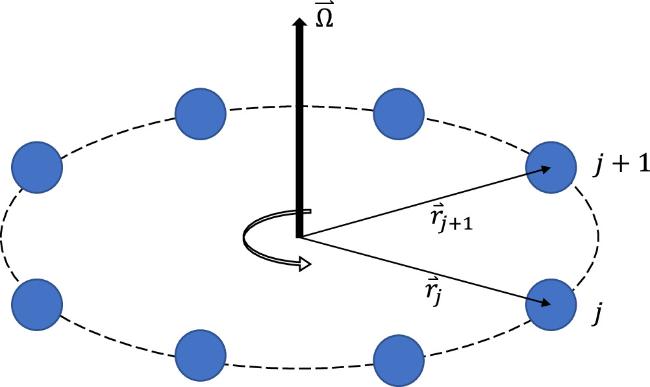
Figure 1. Schematic of the BH model in the rotating reference frame with rotation velocity Ω. |
In order to demonstrate how the rotation velocity affects the quantum phase transition, the mean field theory is adopted where the order parameter is the average of the annihilation operator $\left\langle {\hat{a}}_{j}\right\rangle =\psi $ on the ground state. In this sense, the hopping terms can be written as
$\begin{eqnarray}{\hat{a}}_{j}^{\dagger }{\hat{a}}_{j\pm 1}\to {\hat{a}}_{j}^{\dagger }\left\langle {\hat{a}}_{j\pm 1}\right\rangle +\left\langle {\hat{a}}_{j}^{\dagger }\right\rangle {\hat{a}}_{j\pm 1}-\left\langle {\hat{a}}_{j}^{\dagger }\right\rangle \left\langle {\hat{a}}_{j\pm 1}\right\rangle .\end{eqnarray}$
Eventually the Hamiltonian become the summation of one-body Hamiltonian ${\hat{H}}_{{\rm{l}}{\rm{a}}{\rm{b}}}={\sum }_{j}{H}_{j}$ with $\begin{eqnarray}\begin{array}{rcl}{H}_{j} & = & -\mu {n}_{j}+U{n}_{j}({n}_{j}-1)\\ & & -\,2t\cos \theta \left({\hat{a}}_{j}^{\dagger }\psi +{\psi }^{* }{\hat{a}}_{j}-{\left|\psi \right|}^{2}\right).\end{array}\end{eqnarray}$
According to the Landau phase transition theory, the ground state energy expanded to the forth-order of the order parameter $E={a}_{0}+{a}_{2}{\left|\psi \right|}^{2}+{a}_{4}{\left|\psi \right|}^{4}$ have spontaneous symmetry breaking at the critical point a2 = 0. To analytically determine the ground state and the order parameter simultaneously, we apply the forth-order perturbation theory and obtain the following results
$\begin{eqnarray}{a}_{2}=4{t}^{2}{\cos }^{2}\theta \left(\frac{n+1}{{E}_{n,n+1}}+\frac{n}{{E}_{n,n-1}}\right),\end{eqnarray}$
$\begin{eqnarray}\begin{array}{rcl}{a}_{4} & = & 16{t}^{4}{\cos }^{4}\theta \left[\frac{\left(n+1\right)\left(n+2\right)}{{E}_{n,n+1}^{2}{E}_{n,n+2}}\right.\\ & & +\,\frac{n\left(n-1\right)}{{E}_{n,n-1}^{2}{E}_{n,n-2}}-\frac{{\left(n+1\right)}^{2}}{{E}_{n,n+1}^{3}}-\frac{{n}^{2}}{{E}_{n,n-1}^{3}}\\ & & \left.-\,\frac{n\left(n+1\right)}{{E}_{n,n+1}\,{E}_{n,n-1}^{2}}-\frac{n\left(n+1\right)}{{E}_{n,n+1}^{2}{E}_{n,n-1}}\right],\end{array}\end{eqnarray}$
where ${E}_{n,m}={E}_{n}^{(0)}-{E}_{m}^{(0)}$ is the energy difference between the eigen-states with eigen-energies ${E}_{n}^{(0)}=-\mu n+Un(n-1)$ in the local limit (t = 0).The critical point a2 = 0 determines the phase boundary as
$\begin{eqnarray}\frac{1}{\widetilde{D}}=-\frac{n+1}{\widetilde{\mu }-2n}+\frac{n}{\widetilde{\mu }-2\left(n-1\right)},\end{eqnarray}$
where $\widetilde{\mu }=\frac{\mu }{U}$, $\widetilde{D}=\widetilde{t}\cos \theta $, $\widetilde{t}=\frac{t}{U}$. Above the critical point $\left({a}_{2}\gt 0\right)$ the system stays in the Mott insulator phase with zero order parameter ψ = 0. When getting below the critical point $\left({a}_{2}\lt 0\right)$ the system stays in the superfluid phase with nonzero order parameter $\psi =\sqrt{-{a}_{2}/\left(2{a}_{4}\right)}$, which can be experimentally measured by the critical momentum in the transport measurement.The rotation of the system affects the ground state of the system and eventually shifts the critical point and the phase boundary. The information of the rotation velocity is also contained in the change of the order parameter, which is experimentally measurable. Therefore by measuring the change of the order parameter, we can sense the rotation velocity.
3. Quantum sensing scheme of the rotation velocity
In this section, we propose a quantum sensing scheme of the rotation velocity through the observation of the BH model's quantum phase transition. The phase diagram of the BH model is analytically obtained from equation (9 ), which is shown in figure 2. Here the different phase boundaries correspond to different $\cos \theta $. Since θ is proportional to the rotation velocity, $\cos \theta $ will decreases when the rotation velocity increases. As shown in figure 2, there are several lobes characterized by an integer value of n, in which the ground state of system refers to the Mott insulator. Outside the lobes the nonzero order parameter of the ground state indicates the superfluidity of the system.
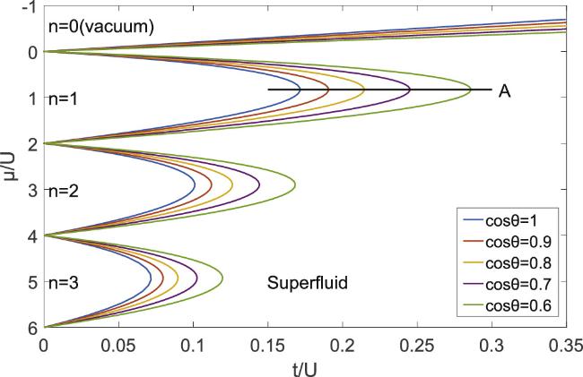
Figure 2. Phase diagram of the BH model under mean field method. Three lobes of different Mott insulators with n = 1, 2, 3 together with the vacuum and the superfluid phase are shown with respect to different Ω. The sensing loop $\widetilde{\mu }=\widetilde{\mu }\left(\widetilde{t},{\rm{\Omega }}\right)$ is given by equation ( |
If the system in an inertial reference is originally prepared in a superfluid state in the vicinity of the phase boundary, then the whole system starts to rotate. The introduction of the rotation velocity results in the expansion of the phase boundary as shown in figure 2. The order parameter shall varies dramatically because of the phase transition from superfluid to Mott insulator. The rotation velocity can be derived by detecting the change of order parameter. Since the rotation velocity only changes the hopping constant from t to $t\cos \theta $, the sensing loop from the superfluid to Mott insulator is a straight line with the constant chemical potential μ, which is also shown as the solid line A in figure 2.
The order parameters $\psi =\psi \left(\tilde{t},{\rm{\Omega }}\right)$ along line A versus the rotation velocity Ω and hopping constant t is shown in figure 3. The order parameter varies dramatically in the vicinity of the phase boundary. By measuring the variance of the order parameter, the rotation velocity can be determined. The variance of the order parameters is also determined by the n-th slope, the variance of the boundary is shown in figure 4. Obviously, the variance of order parameter is more dramatic for higher n, which indicates more efficient sensing scheme in the vicinity of the phase boundary with higher n.
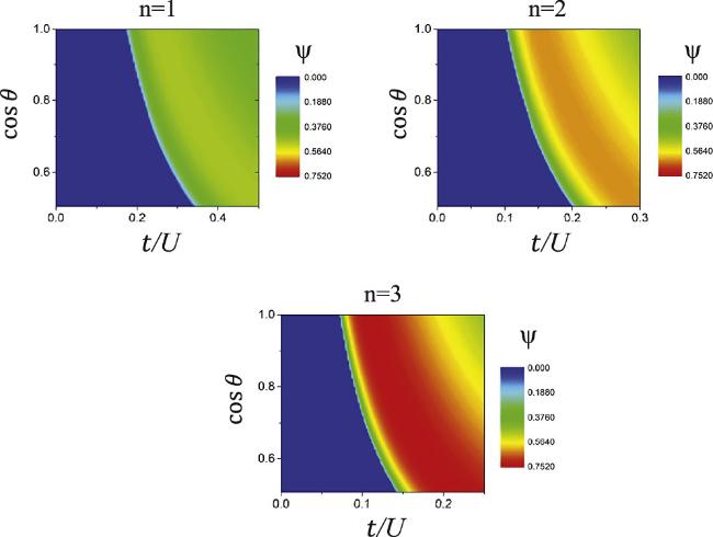
Figure 3. Order parameters $\psi =\psi \left(\tilde{t},{\rm{\Omega }}\right)$ versus t/U and $\cos \theta $, with $\widetilde{\mu }={\widetilde{\mu }}_{0}$, n = 1 (under different Ω). |
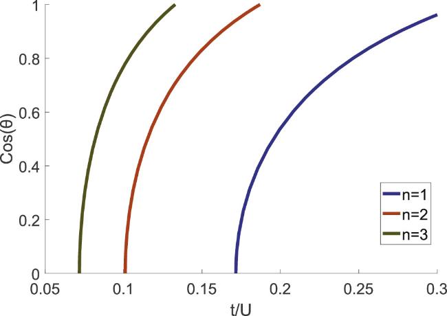
Figure 4. $\cos \theta $ varies with the change of t/U for different n = 1, 2, 3 at μ = nU, which is depicted as blue, red and yellow solid lines. |
Since the BH model has been experimentally demonstrated in the ultracold-atom-based quantum simulators [31–33], the experimental realization of the ring-shaped BH model exactly depends on the one-dimensional ring-shaped optical lattice. Such a closed optical lattice was proposed by taking advantage of the rotational symmetry of Laguerre–Gauss (LG) laser modes [34]. In the rotating reference frame, it should be pointed out that the Peierls phase in equation (4 ) plays an important role in the current quantum sensing scheme. Within certain parameter ranges, it is linearly increasing measurable physical quantities versus the rotation velocity. If we take the rubidium atom in the ultra-cold experiments as an example (m = 1.42 × 10⁻²⁵kg, R = 10−2m, N = 108), the Peierls phase is about 0.27π for a slow rotation velocity Ω = 1rad/s. Secondly, for a relatively large rotation velocity which leads that the Peierls phase is larger than 2π, the scheme can still work by counting the numbers of the phase boundaries which coincides with the phase boundaries without rotating. It is analogy to the shift of the interference fringes between two split laser beams in the optical and laser gyroscopes.
4. The resolution of the quantum sensing scheme
In order to characterize the efficiency of the quantum sensing scheme based on the BH model, the resolution of the sensing scheme with respect to the rotation velocity is obviously important. The resolution can be defined as the full width at half (FWHM) of the change in order parameters, which is defined as
$\begin{eqnarray}{\rm{\Delta }}=\psi \left(\widetilde{\mu },\widetilde{t},n,{\rm{\Omega }}-{\rm{\Delta }}{\rm{\Omega }}\right)-\psi \left(\widetilde{\mu },\widetilde{t},n,{\rm{\Omega }}\right).\end{eqnarray}$
The change in order parameter Δ is caused by the change in rotation velocity (−ΔΩ, 0 ≤ ΔΩ ≤ Ω). When the system is exactly prepared on the phase boundary (a2 = 0), the change in order parameters can be factorized as $\begin{eqnarray}{\rm{\Delta }}=\kappa \left(\widetilde{\mu },n\right)\delta \left(\theta ,{\rm{\Delta }}\theta \right),\end{eqnarray}$
where $\begin{eqnarray}\begin{array}{rcl}\kappa \left(\widetilde{\mu },n\right) & = & \frac{1}{\sqrt{2}}\left[\left(2n-\widetilde{\mu }-3\right)\right.\\ & & \times \,{\left.\left(2n-\widetilde{\mu }+1\right){\left(\widetilde{\mu }+2\right)}^{3}\right]}^{\frac{1}{2}}\\ & & \times \,\left[-24{n}^{4}+48{n}^{3}\left(\widetilde{\mu }+1\right)\right.\\ & & +2n\left(\widetilde{\mu }-10\right)\left(\widetilde{\mu }+1\right)\left(\widetilde{\mu }+2\right)\\ & & +{\left(\widetilde{\mu }+2\right)}^{3}\left(\widetilde{\mu }+3\right)\\ & & {\left.-2{n}^{2}\left(\widetilde{\mu }\left(13\widetilde{\mu }+16\right)-8\right)\right]}^{-\frac{1}{2}},\end{array}\end{eqnarray}$
$\begin{eqnarray}\begin{array}{rcl}\delta \left(\theta ,{\rm{\Delta }}\theta \right) & = & \cos \theta \sec \left(\theta -{\rm{\Delta }}\theta \right)\\ & & \times \,\sqrt{\left(1-\cos \theta \sec \left(\theta -{\rm{\Delta }}\theta \right)\right)},\end{array}\end{eqnarray}$
with θ = γΩ, Δθ = γΔΩ and $\gamma =\frac{2\pi m{R}^{2}}{N\hslash }.$ It should be pointed out that since $\kappa \left(\widetilde{\mu },n\right)$ is independent of the rotation velocity only $\delta \left(\theta ,{\rm{\Delta }}\theta \right)$ plays an essential role in the resolution. For a fixed θ and fixed Ω, $\delta \left(\theta ,{\rm{\Delta }}\theta \right)$ almost exponentially increases when Δθ increases as shown in figure 5(a). To obtain the resolution analytically, the following approximate fitting formula is adopted as $\begin{eqnarray}\delta \left(\theta ,{\rm{\Delta }}\theta \right)\approx \left(\sqrt{a\left(\theta \right){\rm{\Delta }}\theta }\right)\exp \left(-\sqrt{a\left(\theta \right){\rm{\Delta }}\theta }\right),\end{eqnarray}$
with one dependent fitting parameter $a\left(\theta \right).$ It is shown in figure 5(b) as the dashed lines, which fit the exact change of the order parameters well.In this sense, the $\delta \left(\theta ,{\rm{\Delta }}\theta \right)$ reaches its maximum value δm = e−1 when ${\rm{\Delta }}\theta =a{\left(\theta \right)}^{-1}$. Here, not all maximum value can be exactly obtained because Δθ ≤ θ, which gives rise to the critical point θm ≈ 0.67 and the maximum value of $\delta \left(\theta ,{\rm{\Delta }}\theta \right)$ is
$\begin{eqnarray}{\delta }_{m}=\left\{\begin{array}{ll}b\left(\theta \right)\exp \left(-b\left(\theta \right)\right),\quad & \theta \lt {\theta }_{m},\\ {{\rm{e}}}^{-1},\quad & \theta \geqslant {\theta }_{m}\end{array}\right.\end{eqnarray}$
where $b\left(\theta \right)=\sqrt{a\left(\theta \right)\theta }$. Since the resolution defined as FWHM of the change in order parameters, the resolution ϵ is by the following equation $\delta \left(\theta ,\varepsilon \right)=\frac{{\delta }_{m}}{2}$ which is $\begin{eqnarray}\varepsilon =\left\{\begin{array}{ll}\frac{1}{a{\left(\theta \right)}^{2}}{\rm{P}}{\rm{r}}{\rm{o}}{\rm{d}}{\rm{u}}{\rm{c}}{\rm{t}}\,{\rm{L}}{\rm{o}}{\rm{g}}{\left[-\frac{1}{2}b\left(\theta \right)\exp \left(-b\left(\theta \right)\right)\right]}^{2},\quad & {\rm{\Omega }}\lt {{\rm{\Omega }}}_{m},\\ \frac{1}{a{\left(\theta \right)}^{2}}{\rm{P}}{\rm{r}}{\rm{o}}{\rm{d}}{\rm{u}}{\rm{c}}{\rm{t}}\,{\rm{L}}{\rm{o}}{\rm{g}}{\left[-\frac{1}{2e}\right]}^{2},\quad & {\rm{\Omega }}\geqslant {{\rm{\Omega }}}_{m},\end{array}\right.\end{eqnarray}$
Here the Product Log[z] is the solution of the equation z = xex. 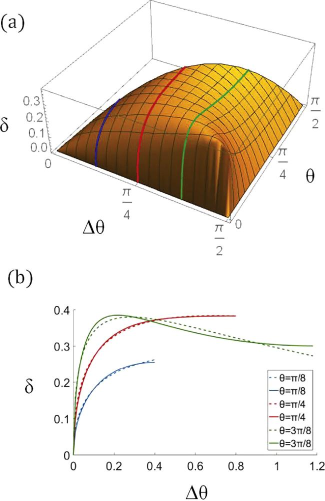
Figure 5. Change of order parameter $\delta \left({\rm{\Omega }},{\rm{\Delta }}{\rm{\Omega }}\right)$ versus the rotation velocity Ω and the change of rotation velocity ΔΩ. The solid lines in (b) denote the exact change of order parameter and the corresponding dashed lines denote the fitting one from equation ( |
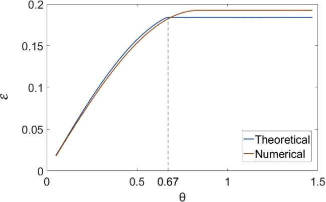
The numerical calculation is shown in figure 6. The red line and blue line represents respectively the rigorous one by solving $\delta \left(\theta ,\varepsilon \right)=\frac{{\delta }_{m}}{2}$ and the fitting one from equation (16 ). As shown in figure 6, the resolution increases when the rotation velocity increases. The approximate resolution fits the rigorous one very well.
Figure 6. The resolution ϵ of the $\delta \left(\theta ,\varepsilon \right)$ versus the Peierls phase θ. The red line and blue line represents respectively the rigorous one by solving $\delta \left(\theta ,\varepsilon \right)=\frac{{\delta }_{m}}{2}$ and the fitting one from equation ( |
5. Conclusion
This work develops a BH model in a rotating frame into consideration due to its Bosonic nature. One reason to choose the BH model is that various phase boundaries between the Mott insulator phase and the superfluid phase emerges due to different occupation numbers. When the unitary transformation is applied to transfer the non-inertial reference frame to an inertial one, the rotation introduces additional phases to the hopping constant between the nearest neighbor sites. It eventually changes the order parameter of BH model, resulting in the changed phase boundary. Therefore it is feasible to obtain the rotation velocity by measuring the changes of the order parameter. Another reason to choose the BH model is that the dramatic change order parameter at the phase transition edges can improve the sensitivity. We propose a sensing scheme of rotation velocity using the QPT of BH model. We find that sensitivity reaches the maximum value at the phase transition edges. Additionally, this sensitivity only depends on the rotation velocity of the rotating reference, the particle number and the ring radius, and it is independent of those parameters of the BH model, such as the hopping constant and the on-site interaction. This work may shed light on the quantum gyroscope using the phase transition edges.