


1. Introduction
Chaos refers to a form of highly complex and erratic behavior that emerges in nonlinear and non-integrable dynamical systems. It is characterized by extreme sensitivity to initial conditions, resulting in inherent unpredictability within such systems. The chaotic behavior reflects the intrinsic randomness present in these systems, as discussed in several studies [1–4]. This chaotic behavior is common in nature. In general relativity, Bombelli and Calzetta showed the existence of chaotic orbits in 1992 when they investigated the geodesic motion around a gravitationally perturbed Schwarzschild black hole [5]. Subsequently, many studies have explored various chaotic dynamics of objects in motion, such as disks and rings, within different spacetime geometries [6–8].
Chaotic phenomena can be verified through various analytical approaches, including Poincaré surface of section analysis, and the Melnikov method, among others. In 1985, the chaotic phenomena was observed in a van der Waals fluid system [9], with the presence of thermal chaos identified by using the Melnikov method [10]. It was demonstrated that when a temporally periodic perturbation is applied within the unstable spinodal region, the van der Waals system exhibits chaotic behavior when the perturbation amplitude exceeds a critical threshold, which depends on the fluid's viscosity. Furthermore, it has been revealed that chaotic behavior always exist under a spatially periodic thermal perturbation.
Since Bekenstein and Hawking demonstrated that black holes can be viewed as thermodynamic objects with temperature [11, 12], it has become widely accepted that black holes can be treated as thermodynamic systems. Utilizing the analogy between black holes and thermodynamic systems, Hawking and Page analyzed the existence of a phase transition between the Schwarzschild-AdS black hole and the thermal AdS space [13]. This well-known Hawking–Page phase transition exhibits characteristics that are similar to the van der Waals solid-liquid phase transition. Within this framework, the critical behavior of the thermodynamics of black holes has progressively been linked to phase transitions in conventional thermodynamic systems. In 2012, Gunasekaran, Kubiznak and Mann introduced the extended phase space for AdS black holes [14], where the cosmological constant Λ was interpreted as a thermodynamical pressure. One of the significant discoveries is the analogy between the P − V criticality of a charged AdS black hole black holes and that of the van der Waals gas-liquid system. The similar P − V critical behaviors are disclosed in the other AdS black hole spacetimes [15–18].
The Melnikov method, previously applied to van der Waals fluids, was extended firstly to analyze chaotic behavior in the extended phase space of thermodynamics of the RN-AdS black holes by Chabab et al [19]. It was proved that the critical amplitude in temporal perturbation depends on the black hole charge. Further generalizations have been explored for charged Gauss–Bonnet-AdS black holes [20], Born–Infeld-AdS black holes [21], charged dilaton-AdS black holes [22], and Bardeen-AdS Black Holes [23]. These studies show distinct dependencies of the critical amplitude on the black hole's parameters such as electric charge, coupling constant and spacetime dimension. Using the Melnikov method, researchers seek to deepen the understanding of black hole thermodynamics, particularly the microstructural interpretation of phase transitions.
Recently, Tang studied the chaotic phenomenon in the extended thermodynamics phase space of Kerr-AdS black holes [24]. It is worth pointing out that the energy definition of Kerr-AdS black holes is an issue. This is because the standard Komar energy expression diverges at infinity. In 2024, Gao et al clarified the origins of different energy definitions of Kerr-AdS black holes and proposed the modified thermodynamics of Kerr-AdS black holes [25]. In this work, we would like to concentrate on the chaotic behavior of the (P, v) section and $({\widehat{{\rm{\Omega }}}}_{H},J)$ section in the extended thermodynamics phase space of Kerr-AdS black holes. In the modified first law of thermodynamics of Kerr-AdS black hole, the modified energy is m/Ξ3/2, which is related to rotating observers [25]. Its thermodynamical properties and P − V criticality have been profoundly studied in [26].
The rest of this paper is organized as follows. In section 2 , we give a brief review to the modified thermodynamics of Kerr-AdS black hole. In section 3 , we discuss the chaos behavior on the (P, $\widehat{V}$) section in the extended thermodynamics phase space of Kerr-AdS black holes under a temporally periodic perturbation in the spinodal region and a spatially periodic perturbation in the equilibrium configuration. In section 4 , the thermal chaos on the $({\widehat{{\rm{\Omega }}}}_{H},J)$ section is investigated. Finally, we present a summary and discussion in section 5 .
2. Modified thermodynamics of Kerr-AdS black hole
In the Boyer–Lindquist coordinate, the Kerr-AdS black hole solution of the vacuum Einstein equations with a cosmological constant Λ is expressed as
$\begin{eqnarray}\begin{array}{rcl}{\rm{d}}{s}^{2} & = & -\frac{{\rm{\Delta }}}{{\rho }^{2}}{\left({\rm{d}}t-\frac{a{\sin }^{2}\theta }{{\rm{\Xi }}}{\rm{d}}\phi \right)}^{2}+\frac{{\rho }^{2}}{{\rm{\Delta }}}{\rm{d}}{r}^{2}\\ & & +\frac{{\rho }^{2}}{{\rm{\Sigma }}}{\rm{d}}{\theta }^{2}+\frac{{\rm{\Xi }}{\sin }^{2}\theta }{{\rho }^{2}}{\left(a{\rm{d}}t-\frac{{r}^{2}+{a}^{2}}{{\rm{\Xi }}}{\rm{d}}\phi \right)}^{2},\end{array}\end{eqnarray}$
where $\begin{eqnarray}\begin{array}{rcl}{\rho }^{2} & = & {r}^{2}+{a}^{2}{\cos }^{2}\theta ,\\ {\rm{\Xi }} & = & 1-\frac{{a}^{2}}{{l}^{2}},\\ {\rm{\Sigma }} & = & 1-\frac{{a}^{2}}{{l}^{2}}{\cos }^{2}\theta ,\\ {\rm{\Delta }} & = & ({r}^{2}+{a}^{2})(1+\frac{{r}^{2}}{{l}^{2}})-2mr.\end{array}\end{eqnarray}$
Here, Λ = −3l−2 is the cosmological constant, m, a are the mass parameter and angular momentum parameter, respectively. The associated thermodynamic quantities are [27]
$\begin{eqnarray}\begin{array}{rcl}T & = & \frac{3{r}_{+}^{4}+({a}^{2}+{l}^{2}){r}_{+}^{2}-{l}^{2}{a}^{2}}{4\pi {l}^{2}{r}_{+}({r}_{+}^{2}+{a}^{2})},\\ S & = & \frac{\pi ({r}_{+}^{2}+{a}^{2})}{{\rm{\Xi }}},\\ {{\rm{\Omega }}}_{H} & = & \frac{a{\rm{\Xi }}}{{r}_{+}^{2}+{a}^{2}},\end{array}\end{eqnarray}$
where r+ represents the horizon radius satisfying Δ(r+) = 0, T, S and ΩH are defined as the Hawking temperature, the Bekenstein–Hawking entropy and the angular velocity respectively. The energy M and the angular momentum J are $M=\frac{m}{{{\rm{\Xi }}}^{2}}$ and $J=\frac{am}{{{\rm{\Xi }}}^{2}}$ respectively.In the framework of the extended phase space for AdS black hole [14], the cosmological constant Λ can be interpreted as a pressure term via the following relation
$\begin{eqnarray}P=-\frac{{\rm{\Lambda }}}{8\pi }.\end{eqnarray}$
The first laws of black hole thermodynamics and the Smarr formula are $\begin{eqnarray}\delta M=T\delta S+{{\rm{\Omega }}}_{H}\delta J+V\delta P,\end{eqnarray}$
$\begin{eqnarray}\frac{M}{2}=TS+{{\rm{\Omega }}}_{H}J-VP,\end{eqnarray}$
where the thermodynamic volume $\begin{eqnarray}V=\frac{4\pi {l}^{2}{r}_{+}({a}^{2}+{r}_{+}^{2})}{3(-{a}^{2}+{l}^{2})}.\end{eqnarray}$
In the recent article [25], the authors proposed a natural criteria to justify the notion of energy. Within the Iyer–Wald formalism, two versions of the first law and the Smarr formula were established for different energies. The difference originated from the choice of the Killing vectors. The standard energy notion m/Ξ2 is associated with the Killing vector $\frac{\partial }{\partial T}=\frac{\partial }{\partial t}+\frac{1}{3}a{\rm{\Lambda }}\frac{\partial }{\partial \phi }$. The relevant thermodynamic quantities, the first law, and the Smarr relation are presented in equations (3 )–(7 ). The other energy notion m/Ξ3/2 is related to the Killing vector $\frac{1}{\sqrt{{\rm{\Xi }}}}\frac{\partial }{\partial t}$, using the notation from [25], the corresponding thermodynamic quantities are
$\begin{eqnarray}{\widehat{{\rm{\Omega }}}}_{H}=\frac{{{\rm{\Omega }}}_{H}}{\sqrt{{\rm{\Xi }}}},\quad \hat{T}=\frac{T}{\sqrt{{\rm{\Xi }}}},\quad \hat{V}=\frac{V}{\sqrt{{\rm{\Xi }}}}.\end{eqnarray}$
The modified first law of black hole thermodynamics is presented as
$\begin{eqnarray}\delta \widehat{M}=\hat{T}\delta S+{\widehat{{\rm{\Omega }}}}_{H}\delta J+\hat{V}\delta P.\end{eqnarray}$
Following the method used in [28], after neglecting all higher order terms of J, one can find that thermodynamics pressure P can be written as
$\begin{eqnarray}\begin{array}{rcl}P & = & \frac{\sqrt[3]{\frac{\pi }{6}}\widehat{T}}{\sqrt[3]{\widehat{V}}}-\frac{1}{2\,{6}^{2/3}\sqrt[3]{\pi }{\widehat{V}}^{2/3}}\\ & & +\frac{2\pi {J}^{2}\left(4\sqrt[3]{6}{\pi }^{2/3}\widehat{T}\sqrt[3]{\widehat{V}}+3\right)}{3{\left(\sqrt[3]{6}{\pi }^{2/3}\widehat{T}{\widehat{V}}^{4/3}+\widehat{V}\right)}^{2}},\end{array}\end{eqnarray}$
where $\widehat{V}$ satisfies $\begin{eqnarray}\widehat{V}=\frac{4\pi {r}_{+}^{3}}{3}+\frac{48\pi {J}^{2}\left(4\pi P{r}_{+}^{2}+1\right)}{{r}_{+}{\left(8\pi P{r}_{+}^{2}+3\right)}^{2}}.\end{eqnarray}$
Defining the specific volume v as $\begin{eqnarray}v=2{\left(\frac{3V}{4\pi }\right)}^{1/3}=2{r}_{+}+\frac{24{J}^{2}\left(4\pi P{r}_{+}^{2}+1\right)}{{r}_{+}^{3}{\left(8\pi P{r}_{+}^{2}+3\right)}^{2}}.\end{eqnarray}$
Thus the thermodynamics pressure P can be rewritten as $\begin{eqnarray}P=\frac{\widehat{T}}{v}-\frac{1}{2\pi {v}^{2}}+\frac{24{J}^{2}(3+4\pi \widehat{T}v)}{\pi {v}^{6}{(1+\pi \widehat{T}v)}^{2}}.\end{eqnarray}$
The abundant phase structures for the modified thermodynamics of the Kerr-AdS black hole have been studied in the extended space [26]. On the (P, v) section in the extended phase space, we plot the graph of $P(v,\widehat{T})$ for fixed J in figure 1. The van der Waals-like phase structure is clearly visualized in this figure.
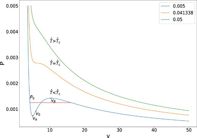
Figure 1. P − v isothermal diagram of the modified thermodynamics of Kerr-AdS black hole with J = 1. The inflection point is v0. The red dashed line with the thermodynamics pressure P0 satisfies the Maxwell's equal area law. This figure is from article [26]. |
Following the critical point condition ${\left.\frac{\partial P}{\partial v}\right|}_{{\widehat{T}}_{C}}\,=0,{\left.\frac{{\partial }^{2}P}{\partial {v}^{2}}\right|}_{{\widehat{T}}_{C}}=0$, we can get
$\begin{eqnarray}{P}_{c}=\frac{0.002}{J},\quad {v}_{c}=6.279{J}^{1/2},\quad {\widehat{T}}_{c}=\frac{0.041}{\sqrt{J}}.\end{eqnarray}$
Furthermore, by using equation (8 ), the functions ${\widehat{{\rm{\Omega }}}}_{H}$, J, $\widehat{T}$ can be expressed as 15 )–(17 ) can be viewed as equations of state of the Kerr-AdS black hole on the (${\widehat{{\rm{\Omega }}}}_{H}$, J) section, i.e., ${\widehat{{\rm{\Omega }}}}_{H}={\widehat{{\rm{\Omega }}}}_{H}(J,\widehat{T})$.
$\begin{eqnarray}J=\frac{3a({a}^{2}+{r}_{+}^{2})(3+8P\pi {r}_{+}^{2})}{2{(3-8{a}^{2}P\pi )}^{2}{r}_{+}},\end{eqnarray}$
$\begin{eqnarray}{\widehat{{\rm{\Omega }}}}_{H}=\frac{2a\sqrt{P(-{a}^{2}+\frac{3}{8P\pi })}\sqrt{\frac{2\pi }{3}}}{{a}^{2}+{r}_{+}^{2}},\end{eqnarray}$
$\begin{eqnarray}\widehat{T}=\frac{\sqrt{\frac{1}{9-24{a}^{2}P\pi }}({a}^{2}(-3+8P\pi {r}_{+}^{2})+3({r}_{+}^{2}+8P\pi {r}_{+}^{4}))}{4\pi {r}_{+}({a}^{2}+{r}_{+}^{2})}.\end{eqnarray}$
Equations (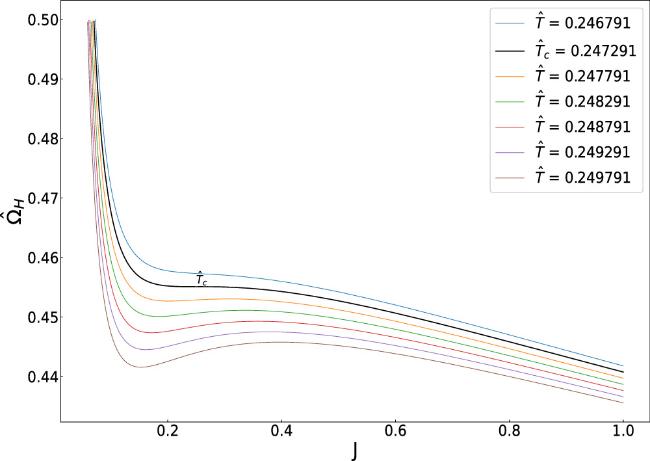
Figure 2. The isotherms of the modified thermodynamics of Kerr-AdS black hole with l = 1 in ${\widehat{{\rm{\Omega }}}}_{H}-J$ plane. Qualitatively, the isotherms near the critical temperature ${\widehat{T}}_{c}$ have similar behavior of Van der Waals system. The black solid line is the critical isotherm. This figure is from article [26]. |
Combining with the equations of state equations (15 )–(17 ), the critical temperature is
$\begin{eqnarray}{\widehat{T}}_{c}^{{\rm{\Omega }}J}=\frac{7(-2+3\sqrt{2})\sqrt{\frac{2P}{9\pi -3\sqrt{2}\pi }}}{{(1+2\sqrt{2})}^{3/2}(-6+5\sqrt{2})}.\end{eqnarray}$
3. Chaos on the (P, v) section in the extended phase space of modified thermodynamics of Kerr-AdS black holes
In this section, we study the chaotic behavior on the (P, v) section in the extended phase space of modified thermodynamics of Kerr-AdS black hole under two types of thermal perturbations.
3.1. Temporal chaos in the spinodal region
When $\widehat{T}\lt {\widehat{T}}_{c}$, the P−v curve in figure 1 can be divided into two stable and one unstable regions. The two points vα and vβ are two extreme points, which satisfy
$\begin{eqnarray}{\left.\frac{\partial P}{\partial v}\right|}_{{v}_{\alpha }}=0,\,{\left.\frac{\partial P}{\partial v}\right|}_{{v}_{\beta }}=0.\end{eqnarray}$
The unstable region [vα, vβ] is named as the spinodal region, the inflection point v0 ∈ [vα, vβ] is determined by $\begin{eqnarray}\frac{{\partial }^{2}P}{\partial {v}^{2}}{\Space{0ex}{3.15ex}{0ex}| }_{{v}_{0}}=0.\end{eqnarray}$
In this subsection, we investigate the temporal chaos in the spinodal region under a weakly temporally periodic perturbation. According to [9, 19–23], we assume the Kerr-AdS black hole flow moves along x-axis in a tube of unit cross section of fixed volume, which includes a total mass 2π/s in a volume 2πv0/s with s a positive parameter. The position of a fluid particle can be described by the Eulerian coordinate x. Let x0 be the Eulerian coordinate of the reference fluid particle. Then the mass M of a column of fluid of unit cross section can be expressed as 27 ), one can obtain
$\begin{eqnarray}M={\int }_{{x}_{0}}^{x}\rho (\xi ,t){\rm{d}}\xi ,\end{eqnarray}$
where ρ(x, t) is the fluid density. In turn, x can be viewed as a function of M and t, i.e., x = x(M, t). From equation ( $\begin{eqnarray*}{x}_{M}(M,t)\equiv \frac{\partial x(M,t)}{\partial M}=\rho {[x(M,t),t]}^{-1}\end{eqnarray*}$
and $\begin{eqnarray*}{x}_{t}(M,t)\equiv \frac{\partial x(M,t)}{\partial t},\end{eqnarray*}$
which are defined as the specific volume v(M, t) and the velocity u(M, t), respectively.The Kerr-AdS black hole flow in the one dimensional can be depicted by the following dynamical system 24 ) into (23 ) yields 25 ) can be reconstructed as
$\begin{eqnarray}\frac{\partial v}{\partial t}=\frac{\partial u}{\partial M},\end{eqnarray}$
$\begin{eqnarray}\frac{\partial u}{\partial t}=\frac{\partial \tau }{\partial M},\end{eqnarray}$
where τ is the Piola stress. According to the van der Waals-Korteweig's capillarity theory, τ is defined as [9] $\begin{eqnarray}\tau =-P(v,\widehat{T})+\mu {u}_{M}-A{v}_{MM}.\end{eqnarray}$
Here A is a positive constant, and μ is a small positive constant viscosity. Substituting ( $\begin{eqnarray}{x}_{tt}=-P{(v,\widehat{T})}_{M}+\mu {u}_{MM}-A{v}_{MMM}.\end{eqnarray}$
Let $\widetilde{M}=sM,\widetilde{t}=st,\widetilde{x}=sx$ and μ = εμ0, equation ( $\begin{eqnarray}{x}_{tt}=-P{(v,\widehat{T})}_{M}+\epsilon s{\mu }_{0}{u}_{MM}-A{s}^{2}{v}_{MMM},\end{eqnarray}$
where ε is a perturbation parameter. Here the overbars have been omitted for later convenience.Now, let us consider the temporal chaos in the spinodal region. The weak time-periodic fluctuation of the absolute temperature near ${\widehat{T}}_{0}$ can be expressed as [9]
$\begin{eqnarray}\widehat{T}={\widehat{T}}_{0}+\epsilon \delta \cos \omega t\cos M,\end{eqnarray}$
with ε ≪ 1, where δ is the amplitude of the perturbation.To perform the perturbation analysis we expand $P(v,\widehat{T})$ around the inflection point $P({v}_{0},{\widehat{T}}_{0})$ in a Taylor series, and to truncate at cubic terms. Therefore we can obtain
$\begin{eqnarray}\begin{array}{rcl}P(v,\widehat{T}) & = & P({v}_{0},{\widehat{T}}_{0})+{P}_{v}({v}_{0},{\widehat{T}}_{0})(v-{v}_{0})\\ & & +{P}_{\widehat{T}}({v}_{0},{\widehat{T}}_{0})(\widehat{T}-{\widehat{T}}_{0})+\frac{1}{2!}{P}_{\widehat{T}\widehat{T}}{(\widehat{T}-{\widehat{T}}_{0})}^{2}\\ & & +{P}_{v\widehat{T}}(v-{v}_{0})(\widehat{T}-{\widehat{T}}_{0})+\frac{1}{3!}{P}_{vvv}{(v-{v}_{0})}^{3}\\ & & +\frac{1}{3!}{P}_{\widehat{T}\widehat{T}\widehat{T}}{(\widehat{T}-{\widehat{T}}_{0})}^{3}+\frac{1}{2}{P}_{vv\widehat{T}}{(v-{v}_{0})}^{2}(\widehat{T}-{\widehat{T}}_{0})\\ & & +\frac{1}{2}{P}_{v\widehat{T}\widehat{T}}(v-{v}_{0}){(\widehat{T}-{\widehat{T}}_{0})}^{2}+...,\end{array}\end{eqnarray}$
where the coefficient ${P}_{vv}({v}_{0},{\widehat{T}}_{0})$ vanishes because $\frac{{\partial }^{2}P(v,{\widehat{T}}_{0})}{\partial {v}^{2}}=0$ at the inflection point v = v0.For simplicity, we only consider the first hydrodynamical mode (x1(t), u1(t)) of the type as 26 ) yields the following dynamical system
$\begin{eqnarray}\begin{array}{rcl}v(M,t) & = & {x}_{M}(M,t)={v}_{0}+{x}_{1}(t)\cos M...,\\ u(M,t) & = & {x}_{t}(M,t)={u}_{1}(t)\sin M....\end{array}\end{eqnarray}$
In the later formulae the subscript 1 will be omitted. The differential equation ( $\begin{eqnarray}\begin{array}{rcl}\dot{x} & = & u,\\ \dot{u} & = & ({P}_{v}-A{s}^{2})x+\epsilon ({P}_{\widehat{T}}+\frac{3{P}_{vv\widehat{T}}}{8}{x}^{2})\delta \cos \omega t+\frac{{P}_{vvv}}{8}{x}^{3}\\ & & -\epsilon {\mu }_{0}su+\frac{3{P}_{vv\widehat{T}}}{8}{\epsilon }^{2}{(\delta \cos \omega t)}^{2}x+\frac{{P}_{\widehat{T}\widehat{T}\widehat{T}}}{8}{\epsilon }^{3}{(\delta \cos \omega t)}^{3}.\end{array}\end{eqnarray}$
By setting z ≡ [x, u]T, the above equations can be organized as $\begin{eqnarray}\dot{z}=f(z)+\epsilon g(z,t)+{\epsilon }^{2}{g}_{1}(z,t)+{\epsilon }^{3}{g}_{2}(z,t),\end{eqnarray}$
where $\begin{eqnarray}f(z)=\left(\begin{array}{cc}u & \\ ({P}_{v}-A{s}^{2})x+\frac{{P}_{\widehat{T}\widehat{T}\widehat{T}}}{8}{x}^{3} & \\ \end{array}\right),\end{eqnarray}$
$\begin{eqnarray}g(z)=\left(\begin{array}{cc}0 & \\ ({P}_{\widehat{T}}+\frac{3{P}_{vv\widehat{T}}}{8}{x}^{2})\delta \cos \omega t-{\mu }_{0}su & \\ \end{array}\right),\end{eqnarray}$
$\begin{eqnarray}{g}_{1}(z)=\left(\begin{array}{cc}0 & \\ \frac{3{P}_{vv\widehat{T}}}{8}{(\delta \cos \omega t)}^{2}x & \\ \end{array}\right),\end{eqnarray}$
and $\begin{eqnarray}{g}_{2}(z)=\left(\begin{array}{cc}0 & \\ \frac{{P}_{\widehat{T}\widehat{T}\widehat{T}}}{8}{(\delta \cos \omega t)}^{3} & \\ \end{array}\right).\end{eqnarray}$
For the unperturbed system (ε = 0), an analytical solution can be obtained $\begin{eqnarray}{z}_{0}(t)=\left(\begin{array}{cc}{x}_{0}(t) & \\ {u}_{0}(t) & \\ \end{array}\right)=\left(\begin{array}{cc}\frac{\pm 4{b}_{1}}{{(-{P}_{vvv})}^{1/2}}{\rm{{\rm{sech}} }}({b}_{1}t) & \\ \frac{\mp 4{b}_{1}^{2}}{{(-{P}_{vvv})}^{1/2}}{\rm{{\rm{sech}} }}({b}_{1}t){\rm{\tanh }}({b}_{1}t) & \\ \end{array}\right).\end{eqnarray}$
Here ${b}_{1}^{2}\equiv \left({P}_{v}-A{s}^{2}\right)$. The solution owns a homoclinic orbit that tends to the saddle point (i.e., the origin point) as t → ± ∞. In figure 3, we plot the two wings of the butterfly-like branches.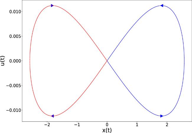
Figure 3. Homoclinic orbit of the unperturbed equations with ${\widehat{T}}_{0}=0.038\lt {\widehat{T}}_{c}$ on the P − v section of the Kerr-AdS black hole. We set J = 1, A = 0.2, s = 0.001. |
Under the temporal perturbation (ε > 0), the above orbit may be destroyed. By employing the Melnikov method, the existence of chaos can be detected. The Melnikov function is given by the following formula [9]37 ) with equations (32 ) and (33 ), one can obtain the Melnikov function for the Kerr-AdS black hole flow
$\begin{eqnarray}M({t}_{0})={\int }_{-\infty }^{\infty }{f}^{T}[{z}_{0}(t-{t}_{0})]{\boldsymbol{J}}g[{z}_{0}(t-{t}_{0})]{\rm{d}}t,\end{eqnarray}$
with $\begin{eqnarray}{\boldsymbol{J}}=\left(\begin{array}{cc}0 & 1\\ -1 & 0\\ \end{array}\right).\end{eqnarray}$
Combining equation ( $\begin{eqnarray}M({t}_{0})\equiv {{I}}_{1}+{{I}}_{2},\end{eqnarray}$
where $\begin{eqnarray}{{I}}_{1}={\int }_{-\infty }^{\infty }{\rm{d}}t\frac{16{\mu }_{0}s{b}_{1}^{4}}{{P}_{vvv}}{{\rm{{\rm{sech}} }}}^{2}{b}_{1}(t-{t}_{0}){{\rm{\tanh }}}^{2}{b}_{1}(t-{t}_{0}),\end{eqnarray}$
and $\begin{eqnarray}\begin{array}{rcl}{{I}}_{2} & = & {\displaystyle \int }_{-\infty }^{\infty }{\rm{d}}t\frac{4{b}_{1}^{2}}{{(-{P}_{vvv})}^{1/2}}\frac{\delta\, {\rm{\sinh }}\,{b}_{1}(t-{t}_{0})}{{{\rm{\cosh }}}^{2}{b}_{1}(t-{t}_{0})}\\ & & \times [\frac{6{b}_{1}^{2}{P}_{vv\widehat{T}}}{{P}_{vvv}}{{\rm{{\rm{sech}} }}}^{2}{b}_{1}(t-{t}_{0})-{P}_{\widehat{T}}]\cos \omega t\\ & = & -\frac{\delta 4{b}_{1}^{2}{P}_{\widehat{T}}}{{(-{P}_{vvv})}^{1/2}}{\displaystyle \int }_{-\infty }^{\infty }{\rm{{\rm{sech}} }}\,{b}_{1}(t-{t}_{0}){\rm{\tanh }}\,{b}_{1}(t-{t}_{0})\cos \omega t{\rm{d}}t\\ & & +\frac{\delta 24{b}_{1}^{4}{P}_{vv\widehat{T}}}{{(-{P}_{vvv})}^{1/2}{P}_{vvv}}{\displaystyle \int }_{-\infty }^{\infty }{{\rm{{\rm{sech}} }}}^{3}{b}_{1}(t-{t}_{0}){\rm{\tanh }}\,{b}_{1}(t-{t}_{0})\cos \omega t{\rm{d}}t\\ & = & -\frac{\delta 4{b}_{1}^{2}{P}_{\widehat{T}}}{{(-{P}_{vvv})}^{1/2}}{{I}}_{3}+\frac{\delta 24{b}_{1}^{4}{P}_{vv\widehat{T}}}{{(-{P}_{vvv})}^{1/2}{P}_{vvv}}{{I}}_{4},\end{array}\end{eqnarray}$
with $\begin{eqnarray}\begin{array}{rcl}{{I}}_{3} & = & {\displaystyle \int }_{-\infty }^{\infty }{\rm{{\rm{sech}} }}\,{b}_{1}(t-{t}_{0}){\rm{\tanh }}\,{b}_{1}(t-{t}_{0})\cos \omega t{\rm{d}}t,\\ {{I}}_{4} & = & {\displaystyle \int }_{-\infty }^{\infty }{{\rm{{\rm{sech}} }}}^{3}{b}_{1}(t-{t}_{0}){\rm{\tanh }}\,{b}_{1}(t-{t}_{0})\cos \omega t{\rm{d}}t.\end{array}\end{eqnarray}$
Next, we will calculate I3 in detail, and the calculation of I4 is similar. Let u = t − t0. Then we have $\begin{eqnarray}\begin{array}{rcl}{{I}}_{3} & = & {\displaystyle \int }_{-\infty }^{\infty }{\rm{{\rm{sech}} }}\,{b}_{1}u{\rm{\tanh }}\,{b}_{1}\,u\,\cos\, \omega u\,\cos\, \omega {t}_{0}{\rm{d}}u\\ & & -{\displaystyle \int }_{-\infty }^{\infty }{\rm{{\rm{sech}} }}\,{b}_{1}\,u\,{\rm{\tanh }}\,{b}_{1}u\,\sin\, \omega u\,\sin\, \omega {t}_{0}{\rm{d}}u\\ & = & \cos \omega {t}_{0}{\displaystyle \int }_{-\infty }^{\infty }{\rm{{\rm{sech}} }}({b}_{1}t)\,{\rm{\tanh }}({b}_{1}t)\,\cos\, \omega t{\rm{d}}t\\ & & -\sin \omega {t}_{0}{\displaystyle \int }_{-\infty }^{\infty }{\rm{{\rm{sech}} }}({b}_{1}t)\,{\rm{\tanh }}({b}_{1}t)\,\sin\, \omega t{\rm{d}}t\\ & \equiv & \cos \omega {t}_{0}{{I}}_{5}-\sin \omega {t}_{0}{{I}}_{6},\end{array}\end{eqnarray}$
with $\begin{eqnarray}\begin{array}{rcl}{{I}}_{5} & = & {\displaystyle \int }_{-\infty }^{\infty }{\rm{{\rm{sech}} }}({b}_{1}t)\,{\rm{\tanh }}({b}_{1}t)\,\cos \omega t{\rm{d}}t,\\ {{I}}_{6} & = & {\displaystyle \int }_{-\infty }^{\infty }{\rm{{\rm{sech}} }}({b}_{1}t){\rm{\tanh }}({b}_{1}t)\sin \omega t{\rm{d}}t.\end{array}\end{eqnarray}$
Considering $\begin{eqnarray}\begin{array}{rcl}f(z) & = & {\rm{{\rm{sech}} }}({b}_{1}z){\rm{\tanh }}({b}_{1}z)\cos \omega z\\ & = & \frac{{\rm{\exp }}({b}_{1}z)-{\rm{\exp }}(-{b}_{1}z)}{{\rm{\exp }}({b}_{1}z)+{\rm{\exp }}(-{b}_{1}z)}[{\rm{\exp }}({\rm{i}}\omega z)+{\rm{\exp }}(-{\rm{i}}\omega z)].\end{array}\end{eqnarray}$
f(z) has an infinite number of second-order limit points in the upper half plane: $\frac{(2k+1)\pi {\rm{i}}}{2{b}_{1}}$, k = 0, 1, 2.... On upper half plane, choose the loop l in figure 4, then $\begin{eqnarray}\begin{array}{rcl}\oint f(z){\rm{d}}z & = & {\displaystyle \int }_{-L}^{L}\frac{{\rm{\exp }}({b}_{1}x)-{\rm{\exp }}(-{b}_{1}x)}{{\rm{\exp }}({b}_{1}x)+{\rm{\exp }}(-{b}_{1}x)}\\ & & \times [{\rm{\exp }}({\rm{i}}\omega x)+{\rm{\exp }}(-{\rm{i}}\omega x)]{\rm{d}}x\\ & & +{\displaystyle \int }_{{l}_{2}}f(z){\rm{d}}z+{\displaystyle \int }_{-L}^{L}\frac{-({\rm{\exp }}({b}_{1}x)-{\rm{\exp }}(-{b}_{1}x))}{{\rm{\exp }}({b}_{1}x)+{\rm{\exp }}(-{b}_{1}x)}\\ & & \times [{\rm{\exp }}({\rm{i}}\omega x-\frac{\pi \omega }{{b}_{1}})+{\rm{\exp }}(\frac{\pi \omega }{{b}_{1}}-{\rm{i}}\omega x)]{\rm{d}}x\\ & & +{\displaystyle \int }_{{l}_{4}}f(z){\rm{d}}z,\end{array}\end{eqnarray}$
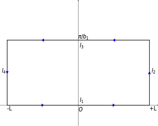
Figure 4. A rectangular closed loop l in the upper half plane. |
Let L → ∞, according to the residue theorem, the right-hand side of the above equation should be equal to 2πi × [the sum of residues of the singularities of function f(z) within the range of $0\lt {\rm{Imz}}\lt \frac{\pi }{{b}_{1}}$]. There is only one second-order singularity $\frac{\pi {\rm{i}}}{2{b}_{1}}$, and yields
$\begin{eqnarray}{\rm{Res}}\,f\left(\frac{\pi {\rm{i}}}{2{b}_{1}}\right)=\frac{\omega }{2{b}_{1}^{2}}\left[{\rm{\exp }}\left(-\frac{\pi \omega }{2{b}_{1}}\right)-{\rm{\exp }}\left(\frac{\pi \omega }{2{b}_{1}}\right)\right]\end{eqnarray}$
Since ${\int }_{{l}_{2}}f(z){\rm{d}}z\to 0$ and ${\int }_{{l}_{4}}f(z){\rm{d}}z\to 0$, as L → ∞, which implies $\begin{eqnarray}\begin{array}{rcl} & & {\displaystyle \int }_{-L}^{L}\frac{{\rm{\exp }}({b}_{1}x)-{\rm{\exp }}(-{b}_{1}x)}{{\rm{\exp }}({b}_{1}x)+{\rm{\exp }}(-{b}_{1}x)}\left[{\rm{\exp }}\left({\rm{i}}\omega x\right)+{\rm{\exp }}\left(-{\rm{i}}\omega x\right)\right]{\rm{d}}x\\ & & +{\displaystyle \int }_{-L}^{L}\frac{-({\rm{\exp }}({b}_{1}x)-{\rm{\exp }}(-{b}_{1}x))}{{\rm{\exp }}({b}_{1}x)+{\rm{\exp }}(-{b}_{1}x)}\\ & & \times \left[{\rm{\exp }}\left({\rm{i}}\omega x-\frac{\pi \omega }{{b}_{1}}\right)+{\rm{\exp }}\left(\frac{\pi \omega }{{b}_{1}}-{\rm{i}}\omega x\right)\right]{\rm{d}}x\\ & & \to 2\pi {\rm{i}}\frac{\omega }{2{b}_{1}^{2}}\left[{\rm{\exp }}\left(-\frac{\pi \omega }{2{b}_{1}}\right)-{\rm{\exp }}\left(\frac{\pi \omega }{2{b}_{1}}\right)\right].\end{array}\end{eqnarray}$
Therefore $\begin{eqnarray*}\begin{array}{rcl} & & {\displaystyle \int }_{-\infty }^{\infty }\frac{{\rm{\exp }}({b}_{1}x)-{\rm{\exp }}(-{b}_{1}x)}{{\rm{\exp }}({b}_{1}x)+{\rm{\exp }}(-{b}_{1}x)}{\rm{\exp }}({\rm{i}}\omega x){\rm{d}}x\\ & = & 2\pi {\rm{i}}\frac{\omega }{{b}_{1}^{2}}\frac{{\rm{\exp }}\left(-\frac{\pi \omega }{2{b}_{1}}\right)}{1+{\rm{\exp }}\left(-\frac{\pi \omega }{{b}_{1}}\right)},\\ & & {\displaystyle \int }_{-\infty }^{\infty }\frac{{\rm{\exp }}({b}_{1}x)-{\rm{\exp }}(-{b}_{1}x)}{{\rm{\exp }}({b}_{1}x)+{\rm{\exp }}(-{b}_{1}x)}{\rm{\exp }}(-{\rm{i}}\omega x){\rm{d}}x\\ & = & -2\pi {\rm{i}}\frac{\omega }{{b}_{1}^{2}}\frac{{\rm{\exp }}\left(\frac{\pi \omega }{2{b}_{1}}\right)}{1+{\rm{\exp }}\left(\frac{\pi \omega }{{b}_{1}}\right)}.\end{array}\end{eqnarray*}$
So we have $\begin{eqnarray*}\begin{array}{rcl}{{I}}_{5} & = & {\displaystyle \int }_{-\infty }^{\infty }\frac{{\rm{\exp }}({b}_{1}x)-{\rm{\exp }}(-{b}_{1}x)}{{\rm{\exp }}({b}_{1}x)+{\rm{\exp }}(-{b}_{1}x)}\left[{\rm{\exp }}({\rm{i}}\omega x)\right.\\ & & \left.+{\rm{\exp }}(-{\rm{i}}\omega x)\right]{\rm{d}}x=0.\end{array}\end{eqnarray*}$
A similar calculation shows $\begin{eqnarray*}\begin{array}{rcl}{{I}}_{6} & = & {\displaystyle \int }_{-\infty }^{\infty }(-{\rm{i}})\frac{{\rm{\exp }}({b}_{1}x)-{\rm{\exp }}(-{b}_{1}x)}{{\rm{\exp }}({b}_{1}x)-{\rm{\exp }}(-{b}_{1}x)}\left[{\rm{\exp }}({\rm{i}}\omega x)\right.\\ & & \left.+{\rm{\exp }}(-{\rm{i}}\omega x)\right]{\rm{d}}x=\frac{2\pi \omega }{{b}_{1}^{2}}\frac{{\rm{\exp }}(\frac{\pi \omega }{2{b}_{1}})}{1+{\rm{\exp }}(\frac{\pi \omega }{{b}_{1}})}.\end{array}\end{eqnarray*}$
Therefore, we have $\begin{eqnarray}\begin{array}{rcl}{{I}}_{3} & = & -\frac{2\pi \omega }{{b}_{1}^{2}}\sin \omega {t}_{0}\frac{{\rm{\exp }}(\frac{\pi \omega }{2{b}_{1}})}{1+{\rm{\exp }}(\frac{\pi \omega }{{b}_{1}})},\\ {{I}}_{4} & = & -\frac{\pi \omega }{3{b}_{1}^{4}}\sin \omega {t}_{0}({\omega }^{2}+{b}_{1}^{2})\frac{{\rm{\exp }}(\frac{\pi \omega }{2{b}_{1}})}{1+{\rm{\exp }}(\frac{\pi \omega }{{b}_{1}})}.\end{array}\end{eqnarray}$
Finally, the Melnikov function can be further expressed as
$\begin{eqnarray}M({t}_{0})=\delta \omega {K}\sin \omega {t}_{0}+{\mu }_{0}s{L},\end{eqnarray}$
with $\begin{eqnarray}\begin{array}{rcl}{K} & = & \frac{8\pi }{{(-{P}_{vvv})}^{1/2}}\left[{P}_{T}-\frac{{P}_{vvT}}{{P}_{vvv}}({\omega }^{2}+{b}_{1}^{2})\right]\frac{{\rm{\exp }}(\frac{\pi \omega }{2{b}_{1}})}{1+{\rm{\exp }}(\frac{\pi \omega }{{b}_{1}})},\\ {L} & = & \frac{32{b}_{1}^{3}}{3{P}_{vvv}}.\end{array}\end{eqnarray}$
The coefficients K and L are depend on the angular momentum parameter a. Moreover, M(t0) will have a simple zero if 30 ) in the phase plane x(t) − u(t). It is shown that as $\delta \lt {\delta }_{c}^{Pv}$, the perturbation system still maintaining a normal butterfly-like trajectory as before. As $\delta \gt {\delta }_{c}^{Pv}$, one can find that the trajectories in the phase plane become unpredictable and complex, and the dynamical evolution of the system occurs chaotic phenomenon.
$\begin{eqnarray}\left|\frac{s{\mu }_{0}{L}}{\delta \omega {K}}\right|\leqslant 1.\end{eqnarray}$
This means that chaotic phenomenon appears if the amplitude of the perturbation δ is larger than the critical value ${\delta }_{c}^{Pv}$, $\begin{eqnarray}{\delta }_{c}^{Pv}=\left|\frac{s{\mu }_{0}{L}}{\omega {K}}\right|.\end{eqnarray}$
In figure 5, we present numerical results of equations of motion (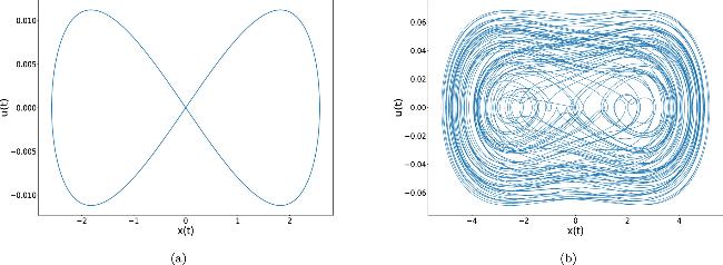
Figure 5. Temporal evolution in x − u plane in the specific temperature ${\widehat{T}}_{0}=0.249291\gt {\widehat{T}}_{c}$: (a) δ = 7.8 × 10⁻⁷ < δc; (b) δ = 0.78 > δc. Parameters are set as ω = 0.01, μ0 = 0.1, J = 1, A = 0.2, s = 0.001. |
The dependence between ${\delta }_{c}^{Pv}$ and black hole parameters is worth surveying in detail. From equation (53 ), one can find that the critical value ${\delta }_{c}^{Pv}$ depends on the angular momentum parameter a. As is shown in figure 6, the critical value ${\delta }_{c}^{Pv}$ is monotonically decreasing with respect to a, which means a larger a leads to the chaotic behavior easier under the time-periodic thermal perturbation.
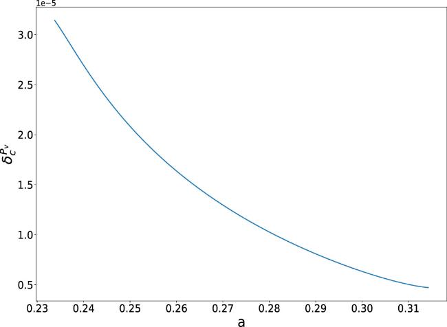
Figure 6. Dependence of the critical value ${\delta }_{c}^{Pv}$ about the angular momentum parameter a. |
3.2. Spatial chaos
In this subsection, we investigate the thermal chaos under a small spatially periodic perturbation. For this purpose, we employ a small spatially periodic perturbation in the equilibrium configuration with an absolute temperature(${\widehat{T}}_{0}\lt {\widehat{T}}_{c}$) expressed in the following form 55 ) yields 56 ) will yield three different types of portraits in the $v-{v}^{{\prime} }$ phase portraits as shown in figures 7–9. The constant B is in the range ${P}_{0}\lt B\lt P({v}_{\beta },{\widehat{T}}_{0})$, one can find that there is a homoclinic orbit connecting the saddle point v = v3 to itself. Similarly, as $P({v}_{\alpha },{\widehat{T}}_{0})\lt B\lt {P}_{0}$, there also exists a homoclinic orbit connecting v1 to itself. However, B = P0, there is a heteroclinic orbit connecting v1 with v3. After adding the perturbation, it is convenient for us to depict the chaotic behavior by using the Melnikov method for these orbits. One can find that dynamical equation (56 ) becomes
$\begin{eqnarray}\widehat{T}={\widehat{T}}_{0}+\epsilon \cos px,\end{eqnarray}$
From van der Waals–Korteweg theory, the stress tensor without flow can be written as $\begin{eqnarray}\tau =-P(v,\widehat{T})-A{v}^{{\prime\prime} },\end{eqnarray}$
where A is a positive constant and the notation ${}^{{\prime} }$ denotes the derivatives with respect to x. For the equilibrium configuration, one can obtain ${\tau }^{{\prime} }=0$, which means that τ = B = constant. Substituting the relation into equation ( $\begin{eqnarray}P(v,\widehat{T})+A{v}^{{\prime\prime} }=B,\qquad -\infty \lt x\lt \infty ,\end{eqnarray}$
where B is the ambient pressure as ∣x∣ → ∞. We first discuss the unperturbed system with $\widehat{T}={\widehat{T}}_{0}$. For any fixed ${\widehat{T}}_{0}\lt {\widehat{T}}_{c}$, equation (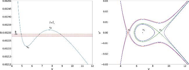
Figure 7. For ${P}_{0}\lt B\lt P({v}_{\beta },{\widehat{T}}_{0})$, P − v diagram and $v-{v}^{{\prime} }$ phase portrait. A homoclinic orbit connecting v3 to itself (the green line). |
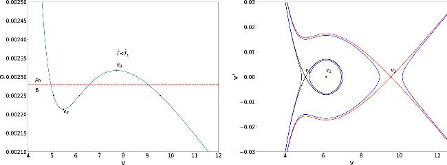
Figure 8. For $P({v}_{\alpha },{\widehat{T}}_{0})\lt B\lt {P}_{0}$, P − v diagram and $v-{v}^{{\prime} }$ phase portrait. A homoclinic orbit connecting v1 to itself (the red line). |
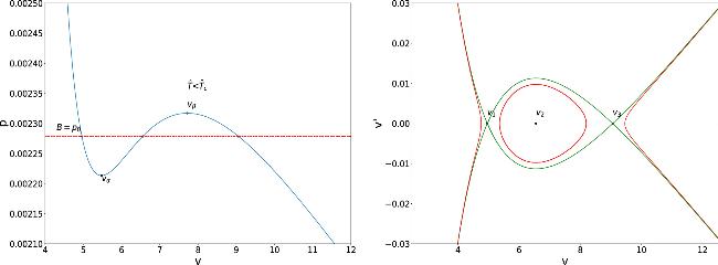
Figure 9. For B = P0, P − v diagram and $v-{v}^{{\prime} }$ phase portrait. A heteroclinic orbit connecting v1 with v3 (the green line). |
$\begin{eqnarray}\begin{array}{rcl}A{v}^{{\prime\prime} } & + & P(v,{\widehat{T}}_{0})+\frac{\epsilon \cos px}{v}\\ & & -\,\frac{48{J}^{2}(1+2\pi {\widehat{T}}_{0}v)\epsilon \cos px}{{v}^{5}{(1+\pi {\widehat{T}}_{0}v)}^{3}}=B.\end{array}\end{eqnarray}$
Thus, the Melnikov function in this case can be simplified as $\begin{eqnarray}M({x}_{0})\equiv -{{\rm{\Theta }}}_{1}\cos p{x}_{0}+{{\rm{\Gamma }}}_{1}\sin p{x}_{0},\end{eqnarray}$
with $\begin{eqnarray}\begin{array}{rcl}{{\rm{\Theta }}}_{1} & = & {\displaystyle \int }_{-\infty }^{\infty }\left\{\frac{{v}_{0}^{{\prime} }(x-{x}_{0})\cos px}{{v}_{0}(x-{x}_{0})}\right.\\ & & \left.+\frac{48{J}^{2}(1+2\pi {\widehat{T}}_{0}{v}_{0})\cos px}{A{[{v}_{0}(x-{x}_{0})]}^{5}{(1+\pi {\widehat{T}}_{0}[{v}_{0}(x-{x}_{0})])}^{3}}\right\}{\rm{d}}x,\end{array}\end{eqnarray}$
$\begin{eqnarray}\begin{array}{rcl}{{\rm{\Gamma }}}_{1} & = & {\displaystyle \int }_{-\infty }^{\infty }\left\{\frac{{v}_{0}^{{\prime} }(x-{x}_{0})\sin px}{{v}_{0}(x-{x}_{0})}\right.\\ & & \left.+\frac{48{J}^{2}(1+2\pi {\widehat{T}}_{0}{v}_{0})\sin px}{A{[{v}_{0}(x-{x}_{0})]}^{5}{(1+\pi {\widehat{T}}_{0}[{v}_{0}(x-{x}_{0})])}^{3}}\right\}{\rm{d}}x.\end{array}\end{eqnarray}$
If Θ1 = 0 and Γ1 = 0, M(x0) is equal to zero; if Θ1 ≠ 0 and Γ1 = 0, M(x0) has a simple zero at px0 = (2k + 1)π/2 with $k\in {\mathbb{Z}}$; If Θ1 = 0 and Γ1 ≠ 0, M(x0) has a simple zero at px0 = kπ with $k\in {\mathbb{Z}}$; If Θ1 ≠ 0 and Γ1 ≠ 0, M(x0) has a simple zero at $p{x}_{0}=\arctan ({{\rm{\Theta }}}_{1}/{{\rm{\Gamma }}}_{1})$. Therefore, the Melnikov function possesses simple zeros in any instances. That is to say, there will always be thermal chaos in the equilibrium configuration of the Kerr-AdS black hole flow under the supposed spatial perturbation. In figures 10–12, the time evolution of equation (57 ) is numerically plotted in the $v-{v}^{{\prime} }$ plane.
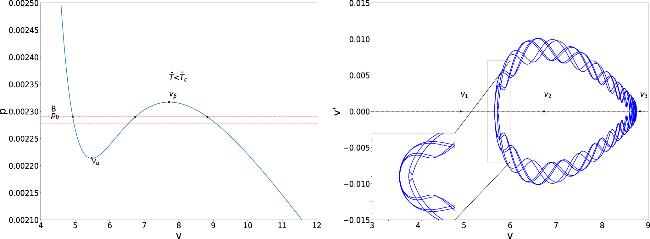
Figure 10. Portrait of the spatial perturbation equation ( |
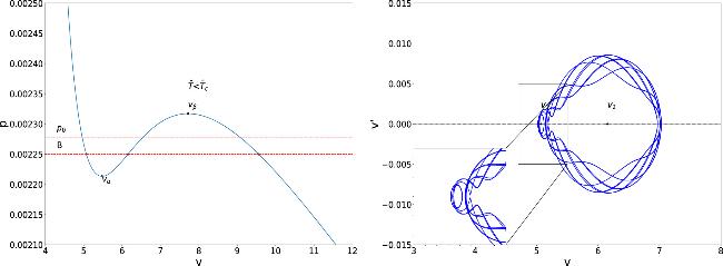
Figure 11. Portrait of the spatial perturbation equation ( |
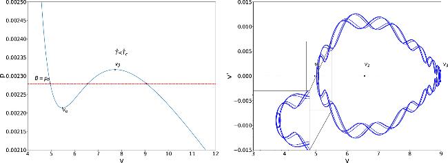
Figure 12. Portrait of the spatial perturbation equation ( |
4. Chaos on the (${\widehat{{\rm{\Omega }}}}_{H}$,J) section in the modified thermodynamics of Kerr-AdS black holes flow under thermal perturbations
In this section, we study the chaotic behavior on the (${\widehat{{\rm{\Omega }}}}_{H}$,J) section in the extended phase space of modified thermodynamics of Kerr-AdS black hole under two types of thermal perturbations.
4.1. Temporal chaos in the spinodal region
On the (${\widehat{{\rm{\Omega }}}}_{H}$, J) section, the equation (26 ) becomes 15 )–(17 ) satisfies $\frac{{\partial }^{2}{\widehat{{\rm{\Omega }}}}_{H}(J,{\widehat{T}}_{0})}{\partial {J}^{2}}=0$ at the inflection point J = J0. Based on the aforementioned similar method, the dynamical equation (26 ) can be further written as
$\begin{eqnarray}{x}_{tt}=-{\widehat{{\rm{\Omega }}}}_{H}{(J,\widehat{T})}_{M}+\epsilon s{\mu }_{0}{u}_{MM}-A{s}^{2}{v}_{MMM}.\end{eqnarray}$
Expanding ${\widehat{{\rm{\Omega }}}}_{H}(J,\widehat{T})$ around the equilibrium point ${\widehat{{\rm{\Omega }}}}_{H}({J}_{0},{\widehat{T}}_{0})$, we have $\begin{eqnarray}\begin{array}{rcl}{\widehat{{\rm{\Omega }}}}_{H}(J,\widehat{T}) & = & {\widehat{{\rm{\Omega }}}}_{H}({J}_{0},{\widehat{T}}_{0})+{({\partial }_{\widehat{J}}{\widehat{{\rm{\Omega }}}}_{H})}_{\widehat{T}}{| }_{0}({J}_{0},{\widehat{T}}_{0})(J-{J}_{0})\\ & & +{({\partial }_{\widehat{T}}{\widehat{{\rm{\Omega }}}}_{H})}_{J}{| }_{0}({J}_{0},{\widehat{T}}_{0})(\widehat{T}-{\widehat{T}}_{0})\\ & & +\frac{1}{2}{({\partial }_{\widehat{T}}^{2}{\widehat{{\rm{\Omega }}}}_{H})}_{J}{| }_{0}({J}_{0},{\widehat{T}}_{0}){(\widehat{T}-{\widehat{T}}_{0})}^{2}\\ & & +{\left({\partial }_{\widehat{T}}{({\partial }_{J}{\widehat{{\rm{\Omega }}}}_{H})}_{\widehat{T}}\right)}_{J}{| }_{0}({J}_{0},{\widehat{T}}_{0})(\widehat{T}-{\widehat{T}}_{0})(J-{J}_{0})\\ & & +\frac{1}{6}{({\partial }_{\widehat{T}}^{3}{\widehat{{\rm{\Omega }}}}_{H})}_{J}{| }_{0}({J}_{0},{\widehat{T}}_{0}){(\widehat{T}-{\widehat{T}}_{0})}^{3}\\ & & +\frac{1}{6}{({\partial }_{J}^{3}{\widehat{{\rm{\Omega }}}}_{H})}_{\widehat{T}}{| }_{0}({J}_{0},{\widehat{T}}_{0}){(J-{J}_{0})}^{3}\\ & & +\frac{1}{2}{\left({\partial }_{\widehat{T}}^{2}{({\partial }_{J}{\widehat{{\rm{\Omega }}}}_{H})}_{\widehat{T}}\right)}_{J}{| }_{0}({J}_{0},{\widehat{T}}_{0}){(\widehat{T}-{\widehat{T}}_{0})}^{2}(J-{J}_{0})\\ & & +\frac{1}{2}{\left({\partial }_{\widehat{T}}{({\partial }_{J}^{2}{\widehat{{\rm{\Omega }}}}_{H})}_{\widehat{T}}\right)}_{J}{| }_{0}({J}_{0},{\widehat{T}}_{0})(\widehat{T}-{\widehat{T}}_{0}){(J-{J}_{0})}^{2},\end{array}\end{eqnarray}$
The absence of ${({\partial }_{J}^{2}{\widehat{{\rm{\Omega }}}}_{H})}_{\widehat{T}}{| }_{0}({J}_{0},{\widehat{T}}_{0})$ is attributed to a fact that the thermodynamics system ( $\begin{eqnarray}\begin{array}{rcl}\dot{x} & = & u,\\ \dot{u} & = & ({({\partial }_{\widehat{J}}{\widehat{{\rm{\Omega }}}}_{H})}_{\widehat{T}}-A{s}^{2})x+\epsilon ({({\partial }_{\widehat{T}}{\widehat{{\rm{\Omega }}}}_{H})}_{J}\\ & & +\frac{3{\left({\partial }_{\widehat{T}}{({\partial }_{J}^{2}{\widehat{{\rm{\Omega }}}}_{H})}_{\widehat{T}}\right)}_{J}}{8}{x}^{2})\delta \cos \omega t+\frac{{({\partial }_{J}^{3}{\widehat{{\rm{\Omega }}}}_{H})}_{\widehat{T}}}{8}{x}^{3}-\epsilon {\mu }_{0}su\\ & & +\frac{3{\left({\partial }_{\widehat{T}}{({\partial }_{J}^{2}{\widehat{{\rm{\Omega }}}}_{H})}_{\widehat{T}}\right)}_{J}}{8}{\epsilon }^{2}{(\delta \cos \omega t)}^{2}x\\ & & +\frac{{({\partial }_{\widehat{T}}^{3}{\widehat{{\rm{\Omega }}}}_{H})}_{J}}{8}{\epsilon }^{3}{(\delta \cos \omega t)}^{3}.\end{array}\end{eqnarray}$
In the case without thermal perturbation (i.e., ε = 0), one can find an analytical solution for the equation (31 ) 64 ) owns the two branches, which corresponds to two wings of butterfly-like orbit shown in figure 13, respectively. Under the time-periodic thermal perturbation (27 ) (i.e., ε ≠ 0), the above homoclinic orbit may break so that the possible chaos could appear in this system. The existence of chaos is determined by the Melnikov function, which has a form
$\begin{eqnarray}{z}_{0}(t)=\left(\begin{array}{c}{x}_{0}(t)\\ {u}_{0}(t))\\ \end{array}\right)=\left(\begin{array}{c}\frac{\pm 4{b}_{2}}{{(-{({\partial }_{J}^{3}{\widehat{{\rm{\Omega }}}}_{H})}_{\widehat{T}})}^{1/2}}{\rm{{\rm{sech}} }}({{\rm{b}}}_{2}{\rm{t}})\\ \frac{\mp 4{b}_{2}^{2}}{{(-{({\partial }_{J}^{3}{\widehat{{\rm{\Omega }}}}_{H})}_{\widehat{T}})}^{1/2}}{\rm{{\rm{sech}} }}({{\rm{b}}}_{2}{\rm{t}}){\rm{\tanh }}({{\rm{b}}}_{2}{\rm{t}}))\\ \end{array}\right).\end{eqnarray}$
Here ${b}_{2}^{2}\equiv \left({({\partial }_{J}{\widehat{{\rm{\Omega }}}}_{H})}_{\widehat{T}})-A{s}^{2}\right)$. It is a homoclinic orbit which joins a saddle equilibrium point to itself. Solution ( $\begin{eqnarray}\begin{array}{rcl}M({t}_{0}) & = & {\displaystyle \int }_{-\infty }^{\infty }{\rm{d}}t\frac{4{b}_{2}^{2}}{{(-{({\partial }_{J}^{3}{\widehat{{\rm{\Omega }}}}_{H})}_{\widehat{T}})}^{1/2}}\frac{\delta \cos \omega t\,{\rm{\sinh }}\,{b}_{2}(t-{t}_{0})}{{{\rm{\cosh }}}^{2}{b}_{2}(t-{t}_{0})}\\ & & \times \left[\frac{6{b}_{2}^{2}{\left({\partial }_{\widehat{T}}{({\partial }_{J}^{2}{\widehat{{\rm{\Omega }}}}_{H})}_{\widehat{T}}\right)}_{J}}{{({\partial }_{J}^{3}{\widehat{{\rm{\Omega }}}}_{H})}_{\widehat{T}}}{{\rm{{\rm{sech}} }}}^{2}{b}_{2}(t-{t}_{0})--{({\partial }_{\widehat{T}}{\widehat{{\rm{\Omega }}}}_{H})}_{J}\right]\\ & & +{\displaystyle \int }_{-\infty }^{\infty }{\rm{d}}t\frac{16{\mu }_{0}s{b}_{2}^{4}}{{({\partial }_{J}^{3}{\widehat{{\rm{\Omega }}}}_{H})}_{\widehat{T}}}{{\rm{{\rm{sech}} }}}^{2}{b}_{2}(t-{t}_{0}){{\rm{\tanh }}}^{2}{b}_{2}(t-{t}_{0}).\end{array}\end{eqnarray}$
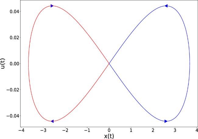
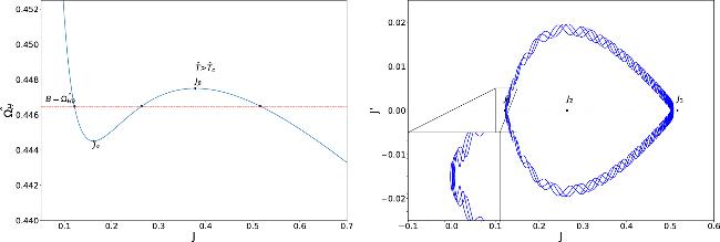
Figure 13. Homoclinic orbit of the unperturbed equations with ${\widehat{T}}_{0}=0.038\lt {\widehat{T}}_{c}$ on the (${\widehat{{\rm{\Omega }}}}_{H}$, J) section of the Kerr-AdS black hole. We set l = 1. |
With the similar calculations, the Melnikov function can be further expressed as
$\begin{eqnarray}M({t}_{0})=\delta \omega {{K}}_{1}\sin \omega {t}_{0}+{\mu }_{0}s{{L}}_{1},\end{eqnarray}$
with $\begin{eqnarray}\begin{array}{rcl}{{K}}_{1} & = & \frac{8\pi }{(-{({({\partial }_{J}^{3}{\widehat{{\rm{\Omega }}}}_{H})}_{\widehat{T}})}^{1/2}}\left[\Space{0ex}{3.55ex}{0ex}{({\partial }_{\widehat{T}}{\widehat{{\rm{\Omega }}}}_{H})}_{J}\right.\\ & & \left.-\frac{{\left({\partial }_{\widehat{T}}{({\partial }_{J}^{2}{\widehat{{\rm{\Omega }}}}_{H})}_{\widehat{T}}\right)}_{J}}{{({\partial }_{J}^{3}{\widehat{{\rm{\Omega }}}}_{H})}_{\widehat{T}}}({\omega }^{2}+{b}_{2}^{2})\right]\frac{{\rm{\exp }}(\frac{\pi \omega }{2{b}_{2}})}{1+{\rm{\exp }}(\frac{\pi \omega }{{b}_{2}})},\\ {{L}}_{1} & = & \frac{32{b}_{2}^{3}}{3{({\partial }_{J}^{3}{\widehat{{\rm{\Omega }}}}_{H})}_{\widehat{T}}}.\end{array}\end{eqnarray}$
The coefficients K1 and L1 are depend on the thermodynamics pressure P in this case. After a simple analysis, one can find that M(t0) has a simple zero if the condition 63 ) numerically. It can be seen that the trajectories exhibit chaotic behaviors if $\delta \gt {\delta }_{c}^{{\rm{\Omega }}J}$, otherwise the perturbation system still keeps the two branches as before. From equation (68 ), one can know that the critical value ${\delta }_{c}^{{\rm{\Omega }}J}$ depends on the cosmological parameter l. Figure 15 shows that ${\delta }_{c}^{{\rm{\Omega }}J}$ is decreasing with l, which means a larger l values lower the threshold for chaos.
$\begin{eqnarray}\delta \geqslant {\delta }_{c}^{{\rm{\Omega }}J}\equiv \left|\frac{s{\mu }_{0}{{L}}_{1}}{\delta \omega {{K}}_{1}}\right|,\end{eqnarray}$
is satisfied. In figure 14, we plot the evolution of the equations of motion (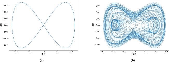
Figure 14. Temporal evolution in x − u plane in the specific temperature ${\widehat{T}}_{0}=0.249291\gt {\widehat{T}}_{c}$: (a) δ = 2.257 × 10⁻⁷ < δc; (b) δ = 0.3 > δc. Parameters are set as ω = 0.01, μ0 = 0.1, l = 1, A = 0.2, s = 0.001. |
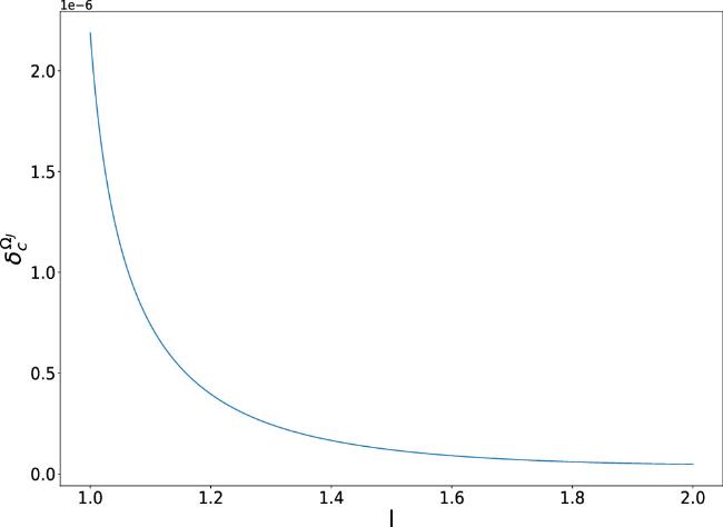
Figure 15. Dependence of the critical value $\delta \lt {\delta }_{c}^{{\rm{\Omega }}J}$ about the cosmological parameter l. |
4.2. Spatial chaos
Based on a small periodic perturbation (54 ), one can find that the dynamical equation (56 ) becomes 69 ), the general solution depicting the homoclinic or heteroclinic orbit can be expressed as 74 ) becomes 70 ) in $J-{J}^{{\prime} }$ phase plane are presented in figures 16–18.
$\begin{eqnarray}A{v}^{{\prime\prime} }+{\widehat{{\rm{\Omega }}}}_{H}(J,{\widehat{T}}_{0})+\frac{\partial {\widehat{{\rm{\Omega }}}}_{H}}{{\partial }_{\widehat{T}}}{| }_{J}(J,{\widehat{T}}_{0})\epsilon \cos px={B}_{1}.\end{eqnarray}$
This second order differential equation can be changed into two first-order differential equations $\begin{eqnarray}\begin{array}{rcl}{v}^{{\prime} } & = & u,\\ {u}^{{\prime} } & = & \frac{1}{A}[{B}_{1}-{\widehat{{\rm{\Omega }}}}_{H}(J,{\widehat{T}}_{0})]-\frac{1}{A}\frac{\partial {\widehat{{\rm{\Omega }}}}_{H}}{\partial \widehat{T}}{| }_{J}(J,{\widehat{T}}_{0})\epsilon \cos px.\end{array}\end{eqnarray}$
For equation ( $\begin{eqnarray}z=\left[\begin{array}{c}{J}_{0}(x-{x}_{0})\\ {u}_{0}(x-{x}_{0})\end{array}\right],\end{eqnarray}$
and the expression of the f(z(x − x0)) and g(z(x − x0, x)) functions becomes $\begin{eqnarray}f(z(x-{x}_{0}))=\left[\begin{array}{c}{u}_{0}(x-{x}_{0})\\ \frac{{B}_{1}}{A}-\frac{{\widehat{{\rm{\Omega }}}}_{H}({J}_{0}(x-{x}_{0}),{\widehat{T}}_{0})}{A}\end{array}\right],\end{eqnarray}$
$\begin{eqnarray}g(z(x-{x}_{0}),x)=\left[\begin{array}{c}0\\ -\frac{\frac{\partial {\widehat{{\rm{\Omega }}}}_{H}}{\partial \widehat{T}}{| }_{J}({J}_{0}(x-{x}_{0}),{\widehat{T}}_{0})\cos px}{A}\end{array}\right].\end{eqnarray}$
Thus, the Melnikov function on the (${\widehat{{\rm{\Omega }}}}_{H},J$) section can be presented as $\begin{eqnarray}\begin{array}{rcl}M({x}_{0}) & = & {\displaystyle \int }_{-\infty }^{\infty }{f}^{T}[{z}_{0}(t-{t}_{0})]{\boldsymbol{J}}g[{z}_{0}(t-{t}_{0})]{\rm{d}}x\\ & = & {\displaystyle \int }_{-\infty }^{\infty }{v}_{0}^{{\prime} }(x-{x}_{0})\frac{\partial {\widehat{{\rm{\Omega }}}}_{H}}{\partial \widehat{T}}{| }_{J}({J}_{0}(x-{x}_{0}),{\widehat{T}}_{0})\cos px{\rm{d}}x,\end{array}\end{eqnarray}$
Introducing the change of variable R = x − x0, equation ( $\begin{eqnarray}\begin{array}{rcl}M({x}_{0}) & = & {\displaystyle \int }_{-\infty }^{\infty }{v}_{0}^{{\prime} }(R)\frac{\partial {\widehat{{\rm{\Omega }}}}_{H}}{\partial \widehat{T}}{| }_{J}({J}_{0}R,{\widehat{T}}_{0})\cos p(R+{x}_{0}){\rm{d}}R\\ & = & {\displaystyle \int }_{-\infty }^{\infty }{v}_{0}^{{\prime} }(R)\frac{\partial {\widehat{{\rm{\Omega }}}}_{H}}{\partial \widehat{T}}{| }_{J}({J}_{0}R,{\widehat{T}}_{0})\\ & & \times \left\{\cos pR\cos p{x}_{0}-\sin pR\sin p{x}_{0}\right\}{\rm{d}}R\\ & = & -{{\rm{\Theta }}}_{2}\cos p{x}_{0}+{{\rm{\Gamma }}}_{2}\sin p{x}_{0},\end{array}\end{eqnarray}$
with $\begin{eqnarray}{{\rm{\Theta }}}_{2}={\int }_{-\infty }^{\infty }{v}_{0}^{{\prime} }(R)\frac{\partial {\widehat{{\rm{\Omega }}}}_{H}}{\partial \widehat{T}}{| }_{J}({J}_{0}R,{\widehat{T}}_{0})\cos pR{\rm{d}}R,\end{eqnarray}$
$\begin{eqnarray}{{\rm{\Gamma }}}_{2}={\int }_{-\infty }^{\infty }{v}_{0}^{{\prime} }(R)\frac{\partial {\widehat{{\rm{\Omega }}}}_{H}}{\partial \widehat{T}}{| }_{J}({J}_{0}R,{\widehat{T}}_{0})\sin pR{\rm{d}}R.\end{eqnarray}$
Hence, whatever the vales of Θ2 and Γ2, the function M(x0) has simple zero, which implies the existence of thermal chaos in the equilibrium configuration of the Kerr-AdS black hole flow under the supposed spatial perturbation. Portrait of the spatial perturbation dynamical system (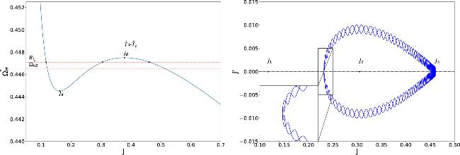
Figure 16. Portrait of the spatial perturbation dynamical system ( |
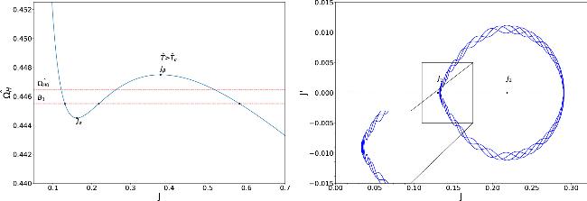
Figure 17. Portrait of the spatial perturbation dynamical system ( |
Figure 18. Portrait of the spatial perturbation dynamical system ( |
5. Conclusions
We have investigated the thermal chaos in the extended phase space of the modified thermodynamics of Kerr-AdS black holes using the Melnikov method. Consistent with the findings obtained in [9], our analysis confirms that chaotic behavior inevitably arises in the unstable spinodal region, regardless of the perturbation type. We calculated the explicit expressions of the critical perturbation amplitude ${\delta }_{c}^{Pv}$ dependent on the angular momentum parameter a for the (P, v) section and ${\delta }_{c}^{{\rm{\Omega }}J}$ dependent on the cosmological parameter l for the $({\widehat{{\rm{\Omega }}}}_{H},J)$ section. For temporal perturbations in the (P, v) section, we find that ${\delta }_{c}^{Pv}$ decreases monotonically with the angular momentum parameter a, indicating that rapidly rotating black holes are more susceptible to chaotic dynamics. Similarly, in the $({\widehat{{\rm{\Omega }}}}_{H},J)$ section, the critical amplitude ${\delta }_{c}^{{\rm{\Omega }}J}$ varies with the cosmological parameter $l=\sqrt{-3/{\rm{\Lambda }}}$ with larger l values lowering the threshold for chaos. These quantitative relations provide a clear criterion for predicting when chaotic behavior will emerge under periodic thermal perturbations. In contrast, for spatially periodic perturbations, chaos persists in both sections irrespective of the perturbation amplitude, reinforcing the universality of chaotic dynamics in the spinodal region.