


1. Introduction
Rapid progress in the development of methods for the generation of ultrashort light pulses and controlling their parameters have been the motivation of achievements in nonlinear optics. Investigations have been done on the propagation of solitons described by a single NLS equation for a scalar field [1–3]. Such solitons also called scalar solitons are formed when a single wave propagates inside a nonlinear medium in a way that maintains its polarization state. When these conditions are not satisfied, one must consider the interaction of several field components at different frequencies or polarizations and simultaneously solve a set of coupled NLS equations [4, 5]. A shape preserving solution of such equations is known as a vector soliton because of its multicomponent nature [3, 6, 7]. It should also be noted that these vector soliton solutions have been demonstrated for the case of a general N-component coupled model with arbitrary nonlinear parameters, as well as multivalley dark soliton solutions with asymmetric or symmetric profiles in multicomponent repulsive Bose–Einstein condensates [8, 9]. In some cases, the soliton constituents correspond to the components of the vector field associated with the soliton [10, 11].
Vector solitons can be derived from incoherent and coherent coupled NLS equations [3, 6, 10]. The difference between the two last pictures is essentially based on the aspect that vector solitons arising from incoherent coupled NLS equations have a coupling that is phase insensitive, which is not the case with those arising from the coherent coupled NLS equation [3, 6, 12]. This last case is an interesting one because information can get lost when propagating via optical fibers. Another important aspect in this study is that vector solitons associated with coherent coupling among optical fields have the coupling dependent on the relative phases of the interacting fields. Here, coherent interaction occurs when the nonlinear medium is weakly anisotropic or weakly birefringent [3, 13]. Coherently coupled vector solitons possess many properties that are different from the case of incoherent coupling [3, 14].
Periodic soliton solution construction for a given evolution of nonlinear partial differential equation, has been extensively central in the study of nonlinear optic phenomena. One of the most important nonlinear models used is the nonlinear Schrodinger equation. There has been outstanding work in the light of obtaining periodic soliton trains solutions [15–18]. A periodic soliton solution, can be seen as a superposition of N-different solution with coinciding centers, it can also be called N-soliton solution. The train of periodic solitons, have a spatially localized structure with a temporal periodic patent. This patent, is significant in nonlinear optics phenomena [16]. In addition, periodic soliton structures were found in photonics crystals wave-guide [17, 18].
In this work, we set as the objective, the dynamic behavior of the periodic train of vector soliton pulses in optical media obtained from a coupled NLS equation, where the effect of the phase parameter is considered. This work is structured as follows: section 1 gives the overall introduction; section 2 presents the mathematics model with their solutions, unveiling the periodic train vector soliton pulses. Section 3 is devoted to the use of the perturbation approach so as to obtain the vector soliton train inducing trapping and reshaping of optical pulses. Lastly, section 4 outlines the concluding remarks.
2. Periodic train vector soliton pulses solution of the coherent coupled NLS equation
Our focus in this section is the determination of the periodic train vector soliton pulses by considering two-component vector solitons formed in planar wave-guides through nonlinear coupling between the TE (Transverse Electric) and TM (Transverse Magnetic) temporal modes. Basically, the propagation of the orthogonally polarized TE and TM wave-guide modes can be obtained using the standard coupled-mode theory as in [19–22]. Using the third-order nonlinear polarization and the third-order susceptibility for a Kerr medium, the polarization components of the TE and TM are separated in to two parts and considering the case of weak birefringence and cubic symmetry far from resonances. Thus, we obtain the normalized equations of evolution for the two orthogonally polarized components expressed as [23–29]1 ) and (2 ) represent the phase sensitive term and is responsible for the coherent coupling, while s1 and s2 characterize the dispersion. Also, the TM component with amplitude B(z, t) is assumed to have a larger propagation constant than the TE component with amplitude A(z, t). In isotropic materials such as optical fibers, σ and α are fixed by the symmetry properties of the susceptibility tensor and in this investigation, they have the value σ = 2/3 and α = 1/3 [23]. Let us recall that when α = 0 and β = 0, the incoherently coupled NLS equation is obtained. The main difference between the incoherently and coherently coupled NLS equations and the vector solitons they describe, is the dynamic energy exchange between the components that occurs for β ≠ 0. The β term result from the birefringence, leads to a phase shift in addition to the nonlinearity induced phase shift. Because of these phase shifts, the coherent coupling term responsible for energy exchange becomes important because of its phase sensitive nature. Thus, the energy exchange leads to a phase-locking effect (i.e. both components of the field can be locked in phase and form a vector soliton) [30]. To solve the above equations, we consider an anomalous dispersion regime (i.e. s1 = s2 = −1) and we look for stationary solutions describing the phase-locking effect in the form1 ) and (2 ), leads to
$\begin{eqnarray}\begin{array}{l}\left({\rm{i}}{\partial }_{z}-\beta -\frac{{s}_{1}}{2}{\partial }_{tt}\right)A+\mu \left[\left({\left|A\right|}^{2}+\sigma {\left|B\right|}^{2}\right)A+\alpha {A}^{* }{B}^{2},],\,{,}=\right]\,0,\end{array}\end{eqnarray}$
$\begin{eqnarray}\begin{array}{l}\left({\rm{i}}{\partial }_{z}-\beta -\frac{{s}_{2}}{2}{\partial }_{tt}\right)B+\mu \left[\left({\left|B\right|}^{2}+\sigma {\left|A\right|}^{2}\right)B+\alpha {B}^{* }{A}^{2}\right]=0,\end{array}\end{eqnarray}$
where the quantities A(z, t) and B(z, t) are the two slow varying fields coupled through their total intensity, with A*(z, t) and B*(z, t) their conjugated complex, z and t are the propagation direction and local time respectively, β is positive and characterizes the degree of birefringence, σ represents the incoherent coupling parameter, α and μ are for the coherent coupling and nonlinear parameters respectively. The last term in equations ( $\begin{eqnarray}A\left(z,t\right)=u\left(t\right)\exp \left[{\rm{i}}\left(qz+{\varphi }_{1}\right)\right],\end{eqnarray}$
$\begin{eqnarray}B\left(z,t\right)=v\left(t\right)\exp \left[{\rm{i}}\left(qz+{\varphi }_{2}\right)\right],\end{eqnarray}$
where u(t) and v(t) govern the shape of the two orthogonally polarized components; q represents the wave number for both components. The shape preserving solutions exist only when the phase difference $\left({\rm{\Delta }}\varphi ={\varphi }_{1}-{\varphi }_{2}\right)$ between the two components takes the values 0; π; ±π/2 [3]. Substituting the above anzats into equations ( $\begin{eqnarray}\frac{1}{2}{\partial }_{tt}u-\left(q+\beta \right)u+\mu \left[{\left|u\right|}^{2}+{\left|v\right|}^{2}\right]u=0,\end{eqnarray}$
$\begin{eqnarray}\frac{1}{2}{\partial }_{tt}v-\left(q+\beta \right)v+\mu \left[{\left|u\right|}^{2}+{\left|v\right|}^{2}\right]v=0.\end{eqnarray}$
For TE, v(t) = 0 and we look for exact nonlocalized solution expressed as
$\begin{eqnarray}{u}_{0}\left(t\right)=\frac{a}{\sqrt{\mu }}\,\rm{dn}\,\left[a\left(t-{t}_{0}\right),k\right].\end{eqnarray}$
In the case of TM, u(t) = 0, looking for nonlocalized solution, we obtain
$\begin{eqnarray}{v}_{0}\left(t\right)=\frac{b}{\sqrt{\mu }}\,\rm{dn}\,\left[b\left(t-{t}_{0}\right),k\right],\end{eqnarray}$
with
$\begin{eqnarray}a=\sqrt{\frac{2\left(q+\beta \right)}{2-{k}^{2}}},\end{eqnarray}$
$\begin{eqnarray}b=\sqrt{\frac{2\left(q-\beta \right)}{2-{k}^{2}}},\end{eqnarray}$
$\begin{eqnarray}q=\frac{{m}^{2}+{p}^{2}}{{m}^{2}-{p}^{2}},\end{eqnarray}$
where m and p are integers such that m ≠ p. This expression establishes a correlation relation between the period of u0(t) and v0(t). Also, it brings out a rich dynamic on the evolution of u0(t) and v0(t).In the last two expressions, dn (. . . ) is the Jacobi Elliptic function of the delta form which describes pulses regularly spaced by periods Tv = 2K(k)/b and Tu = 2K(k)/a, where K(k) is the elliptic integral of the first kind with modulus k (0 < k ≤ 1) characterizing the rate at which the pulses are repeated. Also, the dn() function has a rich profile in that it balances between the nonlinearity and dispersion in the optical fiber. This ensures the existence of a shape preserving, well matched and interacting multiple pulses signal profile [15–18], as can be seen in the figures below. The width of the pulse is determined in these expressions by the birefringence parameter β. We propose that when k = 1, localized solutions are obtained and the expressions are likened to those in [3, 17, 31] for the case of spatial evolution.
Figure 1 presents the intensities of the transverse profiles as time evolves. Each optical intensity [u0(t) or v0(t)] represents the vector sum of all the forces exerted by the electrical or magnetic component of the field at a given point in the field strength. In all the panels of figure 1, we observe that as the phase parameters of the couple (p, m) increases, the intensities of each of the modes increase as well as their number of pulses with respect to time for the TE and TM modes. From figure 1(a), we can notice that the period of mode TM is twice that of TE for the any given time interval. However, the increase of the phase parameters induce an increase of the harmonization time between the two modes. From Figures 1(a)–(f), the TE mode has a very high intensity and has more peaks as compared to that of TM.
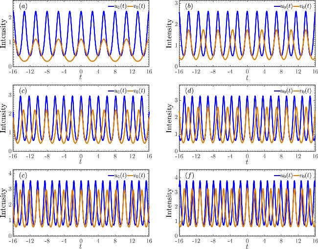
Figure 1. The transverse profile of the intensity u0(t) and v0(t) as a function of time, for stationary mixed mode with repeated linear polarization of the gains propagating in the optical medium, where β = 1; k = 0.98, (p, m = p + 1). Panel (a): p = 1; panel (b): p = 2; panel (c): p = 3; panel (d): p = 4; panel (e): p = 5; and panel (f): p = 6. |
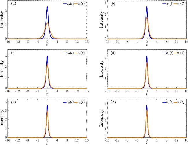
Figure 2. The transverse profile of the intensity u0(t) and v0(t) as a function of time for the parameter k = 1. The other parameters are those of figure 1. |
3. The perturbation approach: vector soliton train induced trapping and reshaping of optical pulses
In the previous paragraph, we have been able to obtain only the scalar train of soliton pulses; but the train of vector soliton pulses are formed when both u(t) and v(t) are nonzero. For these, we perturb our system such that there is a bifurcation from the TE mode. In the vicinity of the bifurcation point (v/u ∼ ϵ ≪ 1); we can now expand u(t) and v(t) in a series in powers of ϵ as [3, 32]
$\begin{eqnarray}u(t)={u}_{0}(t)+{\varepsilon }^{2}{u}_{2}(t),\end{eqnarray}$
$\begin{eqnarray}v(t)=\varepsilon {v}_{1}(t).\end{eqnarray}$
Substituting these expansions in equations (5 ) and (6 ) and linearizing around the exact solution u0(t), we obtain
$\begin{eqnarray}\frac{1}{2}\frac{{\partial }^{2}{v}_{1}}{\partial {t}^{2}}+\left[-\left(q-\beta \right)+\mu {\left|{u}_{0}(t)\right|}^{2}\right]{v}_{1}=0.\end{eqnarray}$
Making use of equations (7 ) and (9a ), we obtain the following eigenvalue equation
$\begin{eqnarray}\frac{{\partial }^{2}{v}_{1}}{\partial {\tau }^{2}}+\left[h\left(q\right)-n\left(n+1\right){k}^{2}{\,\rm{sn}\,}^{2}\left(\tau -{\tau }_{0},k\right)\right]{v}_{1}=0,\end{eqnarray}$
with h(q) = 2 − 2(q − β)/a2, $n\left(n+1\right)=2$ and letting τ = at.Equation (12 ) is the Lamé's equation which reduces to the Legendre equation for the value k = 1, which represents the case of a light beam photon trapped by two interacting pulses and retain their individual shapes [3, 16, 17, 33]. Equation (12 ) has an interesting spectrum, with a great variety of eigenmodes. But the interest here is focused in the determination of a discrete spectrum of eigenmodes, displaying a permanent profile in accordance with their solitonic properties [16, 17, 34, 35].
We would like to point out that the Lamé's equation does not only possess a rich spectrum with a great variety of eigenmodes and energy levels, which display a permanent profile in accordance with their solitonic properties. However, these modes represent exactly the bound states energy levels of the TM component of the amplitude. Equation (12 ) possesses a finite solution only when n is an integer and h(q) has one of the set of 2n + 1 eigenvalues, which are real solutions.
The value of n determines the competition between the Kerr nonlinearity effect and cross-phase modulation effect. When we consider the lowest value of n (i.e. n = 1) which corresponds to the lowest energy level of interaction, we obtain the following family of modes numbered as $\left|n,j\right\rangle $, where j represents the jth number of mode corresponding to a precise family of n.
3.1. Family modes for n = 1
We find:
• $\left|1,0\right\rangle $ soliton mode:
$\begin{eqnarray}{v}_{1}^{1,0}={b}_{0}\,\rm{dn}\,\left(\tau -{\tau }_{0},k\right),\end{eqnarray}$
$\begin{eqnarray}{q}_{1,0}=\beta \left(1-{k}^{2}\right)+1.\end{eqnarray}$
• $\left|1,1\right\rangle $ soliton mode:
$\begin{eqnarray}{v}_{1}^{1,1}={b}_{1}\,\rm{cn}\,\left(\tau -{\tau }_{0},k\right),\end{eqnarray}$
$\begin{eqnarray}{q}_{1,1}=\beta \frac{1-{k}^{2}}{3-{k}^{2}}+\frac{2}{3-{k}^{2}}.\end{eqnarray}$
• $\left|1,2\right\rangle $ soliton mode:13 )–(15 ), display the shape preserving properties of the TM components, which maintains periodic stability structure when passing through the optical medium. Figures 3(b) and (c) depict the intensity of the optical fields ${v}_{1}^{n,j}$ with respect to time τ for k = 0.98 and k = 1, respectively. The first and second mode exhibit soliton train profiles with slightly different intensity levels (for both k = 0.98 and k = 1). Moreover, ${v}_{1}^{1,2}$ of figure 3(b) describes an entanglement of a train of ‘dark' soliton, where for the value k = 1 we can clearly observe a single profile of a topology soliton.
$\begin{eqnarray}{v}_{1}^{1,2}={b}_{2}\,\rm{sn}\,\left(\tau -{\tau }_{0},k\right),\end{eqnarray}$
$\begin{eqnarray}{q}_{1,2}=\beta \frac{1-2{k}^{2}}{3}+\frac{2}{3},\end{eqnarray}$
where μ = 1, b0, b1 and b2 are constants that can be obtained from the normalization condition, k (0 < k ≤ 1) is the Jacobi elliptic modulus which describes interaction of pulses components during propagation in the fiber, such that for small values of k translate an attractive interaction of pulses, whereas high values of k entails repulsive interaction [see Figures 3(b) and (c)]. It also characterizes the frequency at which the radiated TM components, the propagation of the TE components, and also quantifies the gain in amplitude of the pulses in optical fibers over the input pulse. The three modes, equations (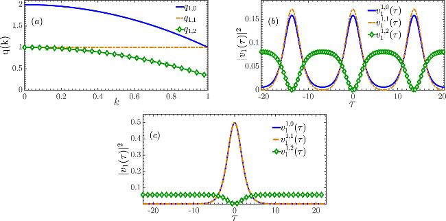
Figure 3. Variation of the modulational wave vector q versus k [panel (a)], as well as the various temporal profiles intensity ${v}_{1}^{2}(\tau )$, obtained respectively for k = 0.98 [panel (b)] and k = 1 [panel (c)]. |
Each qn,j for n = 1, corresponds to the branching of a new periodic train of vector solution with the components $[{u}_{0}(t);{v}_{1}^{n,j}(t)]$, where ${v}_{1}^{n,j}(t)={v}_{1}(t)$. The relative phase of these components is 0 or π which leads to a linearly polarized periodic train of vector solitons. We point out here that, if the two components differ in phase by π/2, they will form an elliptically polarized periodic train of vector solitons. Figure 3(a) illustrates the evolution of the modulational wave vector qn,j with respect to the modulus k. The bottom to the top of figure 3(a) represents the wave vectors of the sn(), dn(), and cn() field modes given by equations (13b ), (14b ) and (15b ). It appears that, in the one soliton limit, the first and second mode reduce to the same single soliton field. This also indicates that, the pulse soliton train will instead be favored at low dispersion.
Figure 4 represents the temporal evolution of the wave intensities for k = 0.98 (left column) and k = 1 (right column). These intensities are the numerical simulation of the Lamé's equation [equation (12 )], with qualitative and quantitative analysis carried out in a single well potential energy, since the total potential energy of the system is periodic [${{ \mathcal E }}_{n}^{p}(\tau ,k)=n(n+1){k}^{2}{\,\rm{sn}\,}^{2}(\tau -{\tau }_{0},k)$]. It can be noticed from this figure that there is a one to one correspondence between the analytical and numerical results, attesting the correctness of both methods. These intensity profiles are induced by phase parameter q. We also observed a very high intensity at the bottom of the potential well, which describes the high amount of localized energy in the well of the potential. This is noticeable during the high data transmission rate in telecommunication.
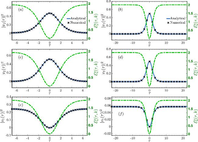
Figure 4. Temporal evolution over one period of ${{ \mathcal E }}_{n}^{p}(\tau ,k)$ of the wave intensities for k = 0.98 (left column ) and for k = 1 (right column) corresponding to the first mode: panels (a) and (b); second mode: panels (c) and (d) and third mode: panels (e) and (f). The analytical solutions are given by equations ( |
Note that restricting the study to a period does not harm the generality as long as the potential in which energy is located remains periodic. Thus, by restricting the numerical analysis of equation (12 ) to a period, it is possible to examine the eigenvectors v1(τ) over this time interval without losing relevant information on the general behavior of the solutions, which can be extended to a wider time range as shown in figure 5.
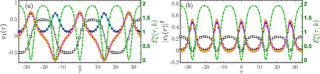
Figure 5. Temporal evolution of the three modes of the wave function v1(τ) [panel (a)] as well as its intensity ∣v1(τ)∣2 [panel (b)] spread out over 5 periods of the potential ${{ \mathcal E }}_{n}^{p}(\tau ,k)$ (green dotted curve), for k = 0.98. The blue, pink and gray color curves respectively represent the analytical curves of the $\left|1,0\right\rangle $, $\left|1,1\right\rangle $ and $\left|1,2\right\rangle $ soliton mode, while the blue crosses, yellow diamond and white squares are those of the numerical solutions. |
The propagation of such high intensity profile signals can significantly impact their transfer due to a down conversion of the input signal in the nonlinear wave-guide. This is manifested in several aspects of the propagating processes, such as the correlation of the matched mode and depends on the phase matching condition in the output spectrum that can be altered by multiple collisions between the optical guiding pulses. Moreover, the rate of entanglement within multi-soliton signals is highly reliant on the robustness of multiplexing processes. In this respect, a good matching of interacting pulses within the sn(), cn() and dn() soliton multiplex has very good means of overcoming such a defect due to their robustness and periodic structure which is relevant in minimizing factors of energy lost. Thus, the structure proposed in this paper is suitable for Wavelength Division Multiplexing (WDM) technology.
Likewise, from equation (10b ) we linearize around the exact solution v0(t) and obtained16 ) represents the Lamé's equation with external optical fields. The homogeneous part of equation (16 ) admits five solution modes, with each having its corresponding energy given as ${h}^{{\prime} }(k)$. They are expressed as follows
$\begin{eqnarray}\begin{array}{l}\frac{{\partial }^{2}{u}_{2}}{\partial {\tau }^{2}}+\left[{h}^{{\prime} }(k)-\varrho (\varrho +1){k}^{2}{\,\rm{sn}\,}^{2}\left(\tau -{\tau }_{0},k\right)\right]{u}_{2}=\,-2\frac{{u}_{0}}{{a}^{2}}{v}_{1}^{2},\end{array}\end{eqnarray}$
where a, u0 and v1 are given above, ϱ(ϱ + 1) = 6. Equation (• $\left|2,0\right\rangle $ soliton mode:
$\begin{eqnarray}{u}_{2}^{2,0}\left(\tau \right)={u}_{2}^{2,0}\,\rm{cn}\,\left(\tau -{\tau }_{0},k\right)\,\rm{dn}\,\left(\tau -{\tau }_{0},k\right),\end{eqnarray}$
$\begin{eqnarray}{h}^{{\prime} }(k)=1+{k}^{2}.\end{eqnarray}$
• $\left|2,1\right\rangle $ soliton mode:
$\begin{eqnarray}{u}_{2}^{2,1}\left(\tau \right)={u}_{2}^{2,1}\,\rm{sn}\,\left(\tau -{\tau }_{0},k\right)\,\rm{dn}\,\left(\tau -{\tau }_{0},k\right),\end{eqnarray}$
$\begin{eqnarray}{h}^{{\prime} }(k)=1+4{k}^{2}.\end{eqnarray}$
• $\left|2,2\right\rangle $ soliton mode:
$\begin{eqnarray}{u}_{2}^{2,2}\left(\tau \right)={u}_{2}^{2,2}\,\rm{sn}\,\left(\tau -{\tau }_{0},k\right)\,\rm{cn}\,\left(\tau -{\tau }_{0},k\right),\end{eqnarray}$
$\begin{eqnarray}{h}^{{\prime} }(k)=4+{k}^{2},\end{eqnarray}$
• $\left|2,3\right\rangle $ soliton mode:
$\begin{eqnarray}\begin{array}{l}{u}_{2}^{2,3}\left(\tau \right)={u}_{2}^{2,3}\left[{\,\rm{sn}\,}^{2}\left(\tau -{\tau }_{0},k\right)-\frac{1+{k}^{2}}{3{k}^{2}}\right.\\ +\left.\frac{\sqrt{1-{k}^{2}\left(1-{k}^{2}\right)}}{3{k}^{2}}\right],\end{array}\end{eqnarray}$
$\begin{eqnarray}{h}^{{\prime} }(k)=2\left[1+{k}^{2}+\sqrt{1-{k}^{2}(1-{k}^{2})}\right],\end{eqnarray}$
• $\left|2,4\right\rangle $ soliton mode:
$\begin{eqnarray}\begin{array}{l}{u}_{2}^{2,4}\left(\tau \right)={u}_{2}^{2,4}\left[{\,\rm{sn}\,}^{2}\left(\tau -{\tau }_{0},k\right)-\frac{1+{k}^{2}}{3{k}^{2}}\right.\\ -\,\left.\frac{\sqrt{1-{k}^{2}\left(1-{k}^{2}\right)}}{3{k}^{2}}\right],\end{array}\end{eqnarray}$
$\begin{eqnarray}{h}^{{\prime} }(k)=2\left[1+{k}^{2}-\sqrt{1-{k}^{2}(1-{k}^{2})}\right].\end{eqnarray}$
Figure 6 highlights the time profiles of the intensity of the five propagation modes ($\left|\varrho ,j\right\rangle $, ϱ = 2 and j = 0, 1, …4) of the homogeneous part (without source term) of equation (14 ). In figure 6, the blue curve refers to the analytical solution given by equations (17a )–(21a ), the cross curve denotes the numerical simulation of equation (14 ) with the corresponding energy ${h}^{{\prime} }(k)$ of each mode, while the green dashed curve represents the periodic potential energy ${{ \mathcal E }}_{\varrho }^{p}(\tau )\,=\varrho (\varrho +1){k}^{2}{\,\rm{sn}\,}^{2}(\tau -{\tau }_{0},k)$. The five modes of this figure are represented respectively, and in order, from top to bottom of each column corresponding to k = 0.98 and k = 1. The almost perfect agreement between the analytical and numerical solution not only corroborates the accuracy of the theoretical study, but also the numerical method used. This correspondence is crucial, because it will be useful when solving equation (14 ) with source term. However, for more inside, we carried out the numerical simulation on a single well potential energy, which by analogy can be replicated all through the system. In the single pulse consideration, the first graph in the right column of figure 6 corresponds to a sech(τ)tanh(τ) when k = 1. However, in the temporal multiplexing consideration, we obtained localized modes (sn(τ)dn(τ)) corresponding with the bound state solution in equation (18a ). By analogy, it can be concluded that the correlation of the center of mass of individual pulses as a reason of their interaction, varies their spectrum internal mode, and includes mode degeneracy. Furthermore, the influence of the optical external source field on the various modes from the inhomogeneous equation (14 ) are numerically illustrated in figure 7.
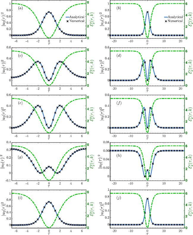
Figure 6. Temporal profile of the wave intensity ∣u2(τ)∣2, solution of the homogeneous part of equation ( |
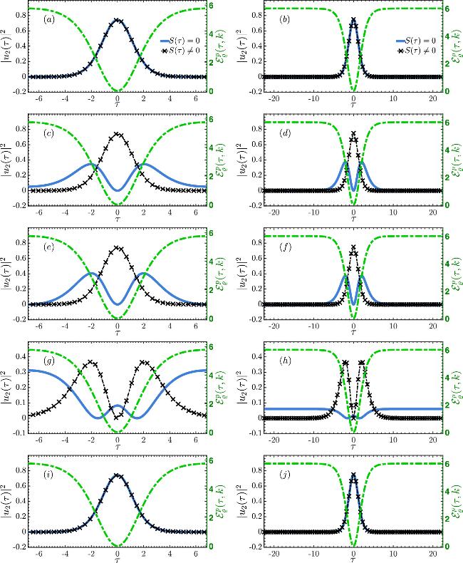
Figure 7. Temporal profile of the intensities of the five modes ∣u2(τ)∣2, solution of the full inhomogeneous equation (14) for k = 0.98 (left hand graph) and k = 1 (right hand graph). The blue curve is that of equation ( |
Figure 7 shows the temporal representation of the intensity profiles of the five modes of equation (14 ). In this figure, we can easily appreciate the influence of the optical field source term S(τ) on the wave functions of the system. This source term is highly dependent on the phase parameter. It should be noted that figure 7 is plotted using the third mode of the homogeneous equation (12 ), namely, equation (15a ). However, the choice of the other modes [first equation (13a ) and second equation (14a )] gives similar results as that of the third mode. A qualitative analysis of figure 7 shows that S(τ) does not considerably influence the wave function of the system for the modes $\left|2,0\right\rangle $ and $\left|2,4\right\rangle $ soliton mode, both for k = 0.98 and for k = 1. This is certainly due to the fact that these modes are degenerate, since they have the same energy $h^{\prime} (k)$. However, it is observed on panels (c)–(h) that the source term has significant qualitative and quantitative influences on the total response of the eigenvalues. Indeed, besides having a very pronounced intensity around τ ≈ 0 (almost twice of the case S(τ) ≈ 0 where the intensity of the wave function has two symmetrical compartments compared to τ ≈ 0) [see panels (c)–(f)], it is observed there that this maximum energy undergoes a modification of configuration accompanied by a reducing factor of 1/2 for the fourth mode of vibration [panels (g) and (h) of figure 7]. The appearance of the external optical field source at the second order of perturbation fuels the self-starting dynamics mechanism such as in micromachining technology. The self preserving nature of the pulse soliton train of the modes $\left|2,0\right\rangle $ and $\left|2,4\right\rangle $ provides effective and efficient long distance communication without losses in the optical wave-guide.
4. Concluding remarks
In conclusion, we have investigated the generation of periodic vector soliton train, where we established that in the anomalous dispersion regime for the coherently coupled NLS equation, the formation and interaction of periodic soliton train pulses arises from slow varying envelop field components propagating in optical media. Their main feature is based on their entangled multiple components propagating together at same group velocity, regardless of the presence of linear effects such as bireferingence and dispersion. Thus, co-propagation is animated by nonlinear interactions which effectively ‘trap' the different components together, constraining them to move as a periodic soliton train. Hence, it is optically pumped through the multiplexing process. The phase-locking effects on the multiplex vector soliton structure was also looked upon. An increase of the phase parameter leads to a narrow band train of vector soliton structure, as well as an increase of the number of pulses. Furthermore, by means of perturbation analysis, we obtained various vector soliton train modes which are multiplex periodic structures suitable in optical communication, microchips technology, optical quantum communication, micromachining applications, etc.