


1. Introduction
What is the most intuitive perception of chaotic motion? A widely accepted understanding involves envisioning chaotic motion as a type of motion resulting from intricate interactions characterized by significant disorder and randomness. Indeed, disorder and randomness are significant characteristics of quantum chaotic systems [1]. In particular, similarity of statistical properties of quantum systems to predictions of the random matrix theory (RMT) has long been used as an indicator of quantum chaos [1–9]. Moreover, it has also been found that eigenstates of quantum chaotic systems exhibit universal properties, with their rescaled components on certain bases following the Gaussian distribution [10–16], in consistency with RMT.
However, disorder and randomness do not fully capture the essence of quantum chaos. Despite the similarity in fluctuation properties described above, quantum chaotic systems deviate from fully random systems described by RMT in various ways. For example, it is well known that average properties, such as averaged spectral density and averaged shape of eigenfunctions (on a given basis), are usually system-dependent and do not show any universal behavior, deviating from RMT.
In this paper, we study distinctions between quantum chaotic systems and RMT from the viewpoint of observable properties, particularly that stated in the framework of the eigenstate thermalization hypothesis (ETH) [17–26]. For observables O on the eigenbasis of the system's Hamiltonian H, the ETH ansatz conjectures that
$\begin{eqnarray}{O}_{ij}=\langle {E}_{i}| O| {E}_{j}\rangle =O({E}_{i}){\delta }_{ij}+f({E}_{i},{E}_{j}){r}_{ij},\end{eqnarray}$
where Ej and ∣Ej⟩ denote eigenvalues and eigenstates of H, respectively. Here, O(Ej) and f(Ei, Ej) are smooth functions of their arguments, δij is the Kronecker Delta function, and ${r}_{ij}={r}_{ji}^{* }$ are random variables with a normal distribution (zero mean and unit variance). Although the ETH remains a hypothesis due to the lack of rigorous proof, most aspects of the ETH have been confirmed by numerical simulations [17, 25, 27–32]. It is now widely accepted that the ETH holds, at least, for quantum chaotic systems when considering few-body observables.As is known, for models associated with dynamical objects, the envelope function f(Ei, Ej) in ETH significantly deviates from RMT predictions [17, 32–38]. We are to show that this deviation stems from correlations in chaotic energy eigenstates, which in turn originate from delicate structures of the Hamiltonians. In particular, such structures are to be studied in the perspective of the underlying dynamical group of the Hamiltonian. In addition, a system-environment uncoupled basis is to be employed for giving certain explanations to the deviations found.
The rest of the paper is organized as follows. In section 2 , examples are given, illustrating the variation of the envelope function f(Ei, Ej) when the Hamiltonians are changed. In section 3 , we analyze the numerical result presented in section 2 from three different aspects. Finally, conclusions and some discussions are given in section 4 .
2. Numerical simulations for the envelope function f(Ei, Ej)
2.1. In a defect Ising chain
We begin with presenting examples of the envelope function f(Ei, Ej). In the following, the eigenstates and eigenvalues of Hamiltonian H are denoted by ∣Ej⟩ and Ej, respectively1 ), the envelope function f(Ei, Ej) is obtained by taking average of the off-diagonal elements,
$\begin{eqnarray}H| {E}_{j}\rangle ={E}_{j}| {E}_{j}\rangle .\end{eqnarray}$
According to the definition in equation ( $\begin{eqnarray}{f}^{2}({E}_{i},{E}_{j})=\overline{| {O}_{ij}^{{\rm{off}}}{| }^{2}}:= \overline{| \langle {E}_{i}| O| {E}_{j}\rangle {| }^{2}},\end{eqnarray}$
for Ei ≠ Ej, over narrow energy shells around Ei and Ej. In our numerical calculations, each energy shell contains approximately 15 levels around Ei and Ej.As the first model, we consider the defect Ising chain (DIS), which consists of N $\frac{1}{2}$-spins subjected to an inhomogeneous transverse field. The Hamiltonian is given by
$\begin{eqnarray}\begin{array}{rcl}{H}_{{\rm{DIS}}} & = & \frac{{B}_{x}}{2}\displaystyle \sum _{l=1}^{N}{\sigma }_{x}^{l}+\frac{{d}_{1}}{2}{\sigma }_{z}^{1}+\frac{{d}_{5}}{2}{\sigma }_{z}^{5}\\ & & +\frac{{J}_{z}}{2}\left(\displaystyle \sum _{l=1}^{N-1}{\sigma }_{z}^{l}{\sigma }_{z}^{l+1}+{\sigma }_{z}^{N}{\sigma }_{z}^{1}\right),\end{array}\end{eqnarray}$
where ${\sigma }_{x,y,z}^{l}$ are Pauli matrices at site l. The parameters are set as Bx = 0.9, d1 = 1.11, d5 = 0.6, and Jz = 1.0. The number of spins in the system is N = 14. Under these parameters, the system is chaotic.In this paper, the spin direct product basis of N $\frac{1}{2}$-spins will be denoted by ∣α⟩, which represents the common eigenstate of all $\{{\sigma }_{z}^{l}\}$. For instance, one such ∣α⟩ can be expressed as
$\begin{eqnarray}| \alpha \rangle =| \uparrow {\rangle }_{1}\otimes | \downarrow {\rangle }_{2}\otimes \cdots \otimes | \uparrow {\rangle }_{N},\end{eqnarray}$
where ∣ ↑ ⟩l and ∣ ↓ ⟩l are eigenstates of ${\sigma }_{z}^{l}$.Figure 1 shows f2(Ei, Ej) as a function of (Ei, Ej) for the observable $O={\sigma }_{x}^{7}$. For a clear view, we show a cross-section at a fixed value of Ej in the inset of figure 1, where a slowly changing plateau is seen at small energy differences ΔE $:= $ ∣Ei − Ej∣, followed by an exponential decay at large ΔE. In fact, as is known in numerical simulations, a slowly changing plateau at small ΔE, which is followed by an exponential decay at large ΔE, is a typical behavior of the f2(Ei, Ej) function in quantum chaotic systems [17, 23, 30, 32, 38–44]. In contrast, in a fully random model whose Hamiltonian matrix is a typical element of the Gaussian Orthogonal Ensemble (GOE), the envelope function f2(Ei, Ej) is flat (as shown in figure 2), without any exponential decay [17].
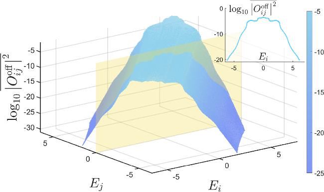
Figure 1. ${\mathrm{log}}_{10}\overline{| {O}_{ij}^{{\rm{off}}}{| }^{2}}$ versus (Ei, Ej) in the DIS model for the observable $O={\sigma }_{x}^{7}$. The inset shows a cross-section taken at Ej = − 0.0013 (indicated by the yellow plane). |
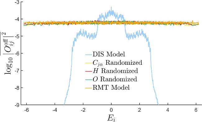
Figure 2. ${\mathrm{log}}_{10}\overline{| {O}_{ij}^{{\rm{off}}}{| }^{2}}$ in different cases. The blue line is an enlargement of the cross-section shown in figure 1. The yellow line represents a cross-section of ${\mathrm{log}}_{10}\overline{| \langle {E}_{i}^{(R)}| O| {E}_{j}^{(R)}\rangle {| }^{2}}$, where $| {E}_{j}^{(R)}\rangle $ is defined in equation ( |
It is worth noting that not just GOE random matrix Hamiltonian can produce eigenstates with disruption of correlations sufficient to flatten the f2(Ei, Ej) function. The red line in figure 2 shows the f2(Ei, Ej) of another system, where the observable O is again taken as $O={\sigma }_{x}^{7}$, but the Hamiltonian H is randomized from the original Hamiltonian of the DIS model as follows. That is, the randomized Hamiltonian H(R) is generated by the following method
$\begin{eqnarray}\langle \alpha | {H}^{(R)}| \beta \rangle ={r}_{\alpha \beta }\langle \alpha | {H}_{{\rm{DIS}}}| \beta \rangle ,\end{eqnarray}$
where rαβ = rβα are independent random numbers drawn from a Gaussian distribution. This operation retains all zero elements of the matrix ⟨α∣H∣β⟩, as well as the average magnitudes of ∣⟨α∣H∣β⟩∣. In other words, the main structural features of HDIS are preserved (as shown in figure 3).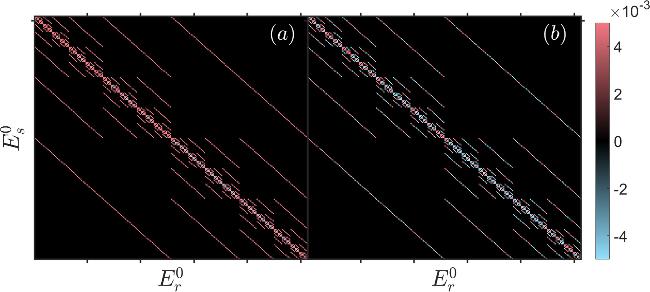
Figure 3. The matrix elements of the original DIS Hamiltonian HDIS (defined in equation ( |
Note that, since the original Hamiltonian HDIS of the DIS model has a sparse matrix in the ∣α⟩-representation, the number of random parameters contained in H(R) is much less than that in a GOE random matrix. However, despite retaining the main structural features of HDIS and containing far less random parameters than a GOE random matrix, figure 2 shows that these random parameters are still enough to disrupt the correlations between eigenstates and observables and further flatten the f2(Ei, Ej) function.
2.2. For two types of Hamiltonians
In this section, we show that the behavior of the envelope function f(Ei, Ej) is closely related to dynamical structure of the Hamiltonian. Concretely, it is shown that, when the Hamiltonian contains only local interactions involving adjacent particles, the f(Ei, Ej) functions have an exponential decay at large ΔE. On the contrary, once numerous non-local interactions enter the Hamiltonian, the exponential decay of f(Ei, Ej) will disappear. For this purpose, we are to study two types of Hamiltonians.
In the first type of Hamiltonian, indicated as ${H}_{n}^{{\rm{DIS}}}$, is obtained by adding second-neighboring interaction and so on to the DIS Hamiltonian. More exactly, it is written as
$\begin{eqnarray}{H}_{n}^{{\rm{DIS}}}={H}_{{\rm{DIS}}}+\displaystyle \sum _{k=1}^{n}{V}_{k},\end{eqnarray}$
where V1 = 0, and Vk(k ≥ 2) represents the sum of all adjacent n-point interactions along x direction. For example, $\begin{eqnarray}{V}_{2}=\displaystyle \sum _{l=1}^{N}{J}_{x}^{l,(l+1)}{\sigma }_{x}^{l}{\sigma }_{x}^{l+1},\end{eqnarray}$
$\begin{eqnarray}\begin{array}{rcl}{V}_{3} & = & \displaystyle \sum _{l=1}^{N}{J}_{x}^{l,(l+1),(l+2)}{\sigma }_{x}^{l}{\sigma }_{x}^{l+1}{\sigma }_{x}^{l+2},\\ & & \cdots \end{array}\end{eqnarray}$
In the above expressions, modulo N is taken for indices exceeding N, and the coefficients $\{{J}_{x}^{l,(l+1)},{J}_{x}^{l,(l+1),(l+2)}\}$ are independent Gaussian random numbers with mean zero. Thus, by definition, ${H}_{n}^{{\rm{DIS}}}$ only contain local interactions.
Figure 4 depicts behaviors of f2(Ei, Ej) obtained from different Hamiltonians ${H}_{n}^{{\rm{DIS}}}$. The observable O is also set as $O={\sigma }_{x}^{7}$. It can be seen that an exponential decay always exists.
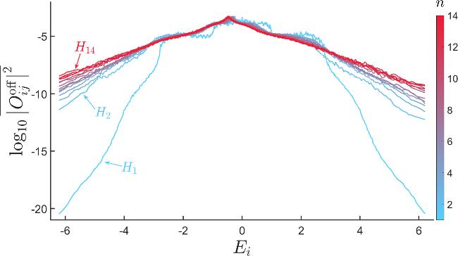
Figure 4. ${\mathrm{log}}_{10}\overline{| {O}_{ij}^{{\rm{off}}}{| }^{2}}$ computed using modified DIS models, which incorporate varying numbers of independent parameters in their Hamiltonians Hn. NR represents the number of independent parameters. Under all these conditions, the observable O is consistently set as $O={\sigma }_{x}^{7}$. For all cross-sections, the energy Ej is fixed at the central value of the respective spectra. |
It is important to point out that, although the interacting strength coefficients $\{{J}_{x}^{l,(l+1)},\,{J}_{x}^{l,(l+1),(l+2)},\cdots \,\}$ are taken as random numbers in our numerical calculations, the behavior of f2(Ei, Ej) are actually not sensitive to the randomness of these coefficients. Even if $\{{J}_{x}^{l,(l+1)},\,{J}_{x}^{l,(l+1),(l+2)},\cdots \,\}$ are taken as equal constants, the result will be similar to that shown in figure 4.
The purpose of studying a second type of system, whose Hamiltonian is indicated as ${H}_{{N}_{R}}^{(R)}$, is to give further study for effects of the randomization introduced to the Hamiltonian H(R) in equation (6 ). For this purpose, we divide the set of the elements of HDIS into NR subsets, which possess an equal number of elements, and, then, multiply each subset by a random number. For example, in the case of NR = 2, a first half of the matrix of HDIS is multiplied by a random number, meanwhile, the second half is multiplied by another random number. Note that the above procedure does not change zero elements of the matrix of HDIS. And, when NR reaches its maximum value NR = 2N−1 × N, ${H}_{{N}_{R}={2}^{N-1}\times N}^{(R)}$ will be the same as the randomized Hamiltonian H(R) in equation (6 ).
Figure 5 depicts the behavior of f2(Ei, Ej) obtained from different ${H}_{{N}_{R}}^{(R)}$. It shows that, with the increase of NR, the exponential-decay behavior of f2(Ei, Ej) is gradually disrupted. This is in contrast to what has been observed in the first type of Hamiltonian.
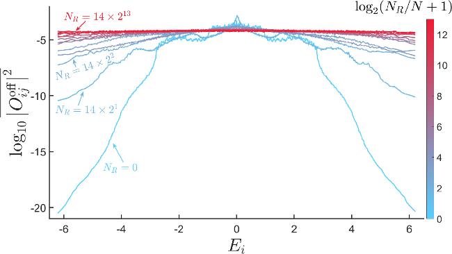
Figure 5. ${\mathrm{log}}_{10}\overline{| {O}_{ij}^{{\rm{off}}}{| }^{2}}$ computed using modified DIS models, which incorporate varying numbers of independent parameters in their Hamiltonians. NR represents the number of independent parameters. Under all these conditions, the observable O is consistently set as $O={\sigma }_{x}^{7}$. For all cross-sections, the energy Ej is fixed at the central value of the respective spectra. |
3. Further understanding for the numerical results
In this section, we give discussions, which are useful for understanding the numerical results discussed above.
3.1. Correlations in chaotic eigenfunctions
In this section, we study the connection between the exponential decay of f2(Ei, Ej) at large ΔE, which has been discussed above, and correlations between eigenstates and the observable.
To this end, we expand the energy eigenstates ∣Ej⟩ of the DIS model in the spin direct product basis {∣α⟩} (which is also the eigenbasis of the observable of interest ${\sigma }_{z}^{l}$) as follows
$\begin{eqnarray}| {E}_{j}\rangle =\displaystyle \sum _{\alpha }{C}_{j\alpha }| \alpha \rangle ,\end{eqnarray}$
where Cjα are real numbers. We also study ‘randomized wavefunctions', denoted by $| {E}_{j}^{(R)}\rangle $, $\begin{eqnarray}| {E}_{j}^{(R)}\rangle =\displaystyle \sum _{\alpha }{{\rm{e}}}^{{\rm{i}}{\theta }_{j\alpha }^{(R)}}| {C}_{j\alpha }| | \alpha \rangle ,\end{eqnarray}$
where ${\theta }_{j\alpha }^{(R)}$ are randomly chosen from the two values of 0 and π. This operation preserves the magnitude of the eigenfunction Cjα while disrupting the phase correlations among the components of the wavefunctions manually.Based on the above construction, we have calculated the matrix elements $\overline{| \langle {E}_{i}^{(R)}| O| {E}_{j}^{(R)}\rangle {| }^{2}}$, where O is again taken as $O={\sigma }_{x}^{7}$. A cross-section of the result is also plotted in figure 2 (yellow line).
Figure 2 shows that, in $\overline{| \langle {E}_{i}^{(R)}| O| {E}_{j}^{(R)}\rangle {| }^{2}}$, the exponential decay at large ΔE disappears, and the f2(Ei, Ej) function becomes similar to the result predicted by the random matrix model. This finding indicates that the correlations among the phases of the original eigenfunctions of the DIS model are crucial for maintaining the exponential decay of the f2(Ei, Ej) function. When these correlations are destroyed, the f2(Ei, Ej) function becomes structureless.
Besides the conditions discussed above, we would also like to point out that the randomization of the observable O can also flatten the f2(Ei, Ej) function. The green line in figure 2 shows the shape of $\overline{| \langle {E}_{i}| {O}^{(R)}| {E}_{j}\rangle {| }^{2}}$, where ∣Ei/j⟩ are energy eigenstates of the original DIS model, and the randomized observable O(R) is constructed as follows:
$\begin{eqnarray}\langle \alpha | {O}^{(R)}| \beta \rangle ={r}_{\alpha \beta }\langle \alpha | {\sigma }_{x}^{7}| \beta \rangle .\end{eqnarray}$
The rαβ = rβα are also independent random numbers drawn from a Gaussian distribution. From figure 2, we can see that in this case, the behavior of the f2(Ei, Ej) function is again close to that in the random matrix model but far from the rapid decay behavior in the original DIS model.The above numerical simulations show that correlations in energy eigenstates and observables are crucial for the non-trivial structure of the envelope function f(Ei, Ej). In particular, f(Ei, Ej) becomes flat (namely, structureless), once such correlations are destroyed.
3.2. Relevance of dynamical group
The numerical results presented in the preceding sections indicate that strong correlations in chaotic eigenfunctions are closely related to the dynamical structure of the Hamiltonian. In this section, we discuss in the perspective of the so-called dynamical group.
As is known, in a model related to dynamical objects, the Hamiltonian H is certain function of the generators of some Lie group, known as the dynamical group. For instance, consider a system involving N $\frac{1}{2}$-spin particles. The Hamiltonian for such a system is a function of operators structured as follows: 13 ) are the four generators of the SU(2) group, while the g-operators in equation (12 ) are generators of the group [SU(2)]N,
$\begin{eqnarray}g={g}^{1}\otimes {g}^{2}\otimes \cdots \otimes {g}^{l}\otimes \cdots \otimes {g}^{N},\end{eqnarray}$
where gl represents one of the four possible operators $\begin{eqnarray}{g}^{l}={\sigma }_{x}^{l},{\sigma }_{y}^{l},{\sigma }_{z}^{l},\,\rm{or}\,{I}^{l},\end{eqnarray}$
with ${\sigma }_{x,y,z}^{l}$ the Pauli matrices and Il the identity operator at site l. The four operators in equation ( $\begin{eqnarray}{[SU(2)]}^{N}:= \mathop{\underbrace{SU(2)\otimes SU(2)\otimes \cdots \otimes SU(2)}}\limits_{{\rm{Direct}}\,{\rm{product}}\,{\rm{of}}\,N\,{\rm{groups}}}.\end{eqnarray}$
From a physical viewpoint, each group generator g signifies a particular kind of interaction among particles within the system. For example,
$\begin{eqnarray}g={\sigma }_{x}^{1}\otimes {\sigma }_{x}^{2}\otimes {I}^{3}\otimes \cdots \otimes {I}^{N}\end{eqnarray}$
represents the interaction between the first and second spins. The independent parameters mentioned above refer to coefficients of those generators that are used in the construction of the Hamiltonian.Among all the above discussed g-operators, the majority represent non-local interactions. In other words, g-operators that can be included in dynamical models only account for a small portion, whose number is far less than the dimension of the Hilbert space. In such models, all the system's properties, including its eigenstates, should in fact depend only on a small number of generators (operators). Generically, this may imply strong correlations within the eigenstates.
For example, the DIS Hamiltonian HDIS in equation (4 ) is described by (2N + 2) dynamical group generators, meanwhile, as discussed previously, the DIS energy eigenstates exhibit strong correlations, and the corresponding f(Ei, Ej) function have exponential behavior. In contrast, the Hamiltonian of the RMT model incorporates all 4N combinations of the generator g, most of which correspond to quite complex interactions, which disrupted correlations within the eigenstates, and the f(Ei, Ej) function becomes flatten.
Moreover, usually, physical observables O are also generated from a small number of generators of the dynamical group. Indeed, numerical simulations discussed previously show strong correlations between such physical observables O and the DIS Hamiltonian.
3.3. Explanations in uncoupled representation
For the purpose of understanding numerical simulations presented in previous sections, one meaningful question is as follows: is there a special representation, which is of special relevance to the observable O, while, in which the two types of Hamiltonian discussed previously, show qualitatively different types of matrix structure? In this section, we show that a system-environment uncoupled basis is useful for this purpose.
Let us consider a local observable O, which is for a central system ${ \mathcal S }$. The rest of the total system is referred as the environment ${ \mathcal E }$. The total Hamiltonian is written as
$\begin{eqnarray}H={H}_{{ \mathcal S }}+{H}_{{ \mathcal E }}+{H}_{{ \mathcal I }},\end{eqnarray}$
where ${H}_{{ \mathcal S }}$ and ${H}_{{ \mathcal E }}$ denote the Hamiltonians of ${ \mathcal S }$ and ${ \mathcal E }$, respectively, determined under the weak-coupling limit, while ${H}_{{ \mathcal I }}$ represents the interaction Hamiltonian between ${ \mathcal S }$ and ${ \mathcal E }$. The uncoupled system-environment Hamiltonian is written as $\begin{eqnarray}{H}_{0}={H}_{{ \mathcal S }}+{H}_{{ \mathcal E }},\end{eqnarray}$
with eigenvalues and eigenstates indicated as ${E}_{r}^{0}$ and $| {E}_{r}^{0}\rangle $, respectively, in the increasing-energy order, $\begin{eqnarray}{H}_{0}| {E}_{r}^{0}\rangle ={E}_{r}^{0}| {E}_{r}^{0}\rangle .\end{eqnarray}$
The set $\{| {E}_{r}^{0}\rangle \}$ constitutes the system-environment uncoupled basis.In the DIS model, with $O={\sigma }_{x}^{7}$, the seventh spin is taken as the central system ${ \mathcal S }$ and the remaining spins as the environment ${ \mathcal E }$. Thus,
$\begin{eqnarray}{H}_{{ \mathcal S }}=\frac{{B}_{x}}{2}{\sigma }_{x}^{7},\end{eqnarray}$
$\begin{eqnarray}\begin{array}{rcl}{H}_{{ \mathcal E }} & = & \frac{{B}_{x}}{2}\displaystyle \sum _{l\ne 7}{\sigma }_{x}^{l}+\frac{{d}_{1}}{2}{\sigma }_{z}^{1}+\frac{{d}_{5}}{2}{\sigma }_{z}^{5}\\ & & +\frac{{J}_{z}}{2}\left(\displaystyle \sum _{l\ne 6,7}{\sigma }_{z}^{l}{\sigma }_{z}^{l+1}+{\sigma }_{z}^{N}{\sigma }_{z}^{1}\right).\end{array}\end{eqnarray}$
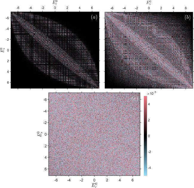
Figure 6 shows schematic plots for structures of the matrix elements of HDIS (figure 6(a)), ${H}_{n=14}^{{\rm{DIS}}}$ (figure 6(b)), and ${H}_{{N}_{R}={2}^{13}\times 14}^{(R)}$ (figure 6(c)) in the system-environment uncoupled basis $| {E}_{r}^{0}\rangle $. It can been seen that significant elements of the Hamiltonians of dynamical models (HDIS and ${H}_{n=14}^{{\rm{DIS}}}$) are confined to a few band-shaped areas, while those the ${H}_{{N}_{R}={2}^{13}\times 14}^{(R)}$ spans almost over all of the basis states.
Figure 6. The matrix elements in the system-environment uncoupled basis $| {E}_{r}^{0}\rangle $. Specifically, panel (a) depicts the matrix elements $\langle {E}_{s}^{0}| {H}_{{\rm{DIS}}}| {E}_{r}^{0}\rangle $, panel (b) illustrates the matrix elements $\langle {E}_{s}^{0}| {H}_{n=14}^{{\rm{DIS}}}| {E}_{r}^{0}\rangle $, and panel (c) shows the matrix elements $\langle {E}_{s}^{0}| {H}_{{N}_{R}={2}^{13}\times 14}^{(R)}| {E}_{r}^{0}\rangle $. Here, the total spin number N = 14. |
Note that since $| {E}_{r}^{0}\rangle $ are eigenstates of H0, all off-diagonal elements of $\langle {E}_{s}^{0}| H| {E}_{r}^{0}\rangle $ come from the system-environment interaction ${H}_{{ \mathcal I }}$. Therefore, the extent of the region occupied by the Hamiltonian in the uncoupled basis $| {E}_{r}^{0}\rangle $ actually reflects a characteristic of the interaction ${H}_{{ \mathcal I }}$.
The above results show that, in the uncoupled basis $| {E}_{r}^{0}\rangle $, the system-environment interaction ${H}_{{ \mathcal I }}$ of a dynamical quantum chaotic system occupies merely a few band-shaped regions of the matrix. This implies strong correlations within energy eigenstates and gives an explanation to the exponential decay of the f2(Ei, Ej) function at large ΔE. Meanwhile, the envelop function is flat for ${H}_{{N}_{R}={2}^{13}\times 14}^{(R)}$.
Finally, it is worth mentioning that perturbation theories offer a natural avenue for connecting energy eigenstates with the system-environment uncoupled basis when treating ${H}_{{ \mathcal I }}$ as a perturbation. For example, a perturbation theory, which gives convergent perturbation expansions for part of the eigenfunction even at strong perturbations [45, 46], may be useful for future investigations concerning the relationship between the matrix structure of ${H}_{{ \mathcal I }}$ in the uncoupled basis and the behavior of the f(Ei, Ej) function.
4. Discussions and conclusions
In this paper, we study the distinctions between dynamical quantum chaotic systems and systems described by RMT manifested in statistical properties of observables. In particular, we investigate the structure of the envelope function f(Ei, Ej), defined within the framework of the ETH. Through numerical simulations, we observe the presence of exponential decay at large ΔE for dynamical systems, and its absence in systems described by RMT. To further unveil the connection between the non-trivial structure of f(Ei, Ej) and the dynamical structure of the system, we investigate two types of Hamiltonians where the dynamical structure can be tuned. Numerical results show that the non-trivial structure of f(Ei, Ej) becomes less prominent as the dynamical structure of the system is disrupted, eventually flattening out.
We provide a framework for understanding the underlying physics behind the numerical observations above, which is presented from the following three perspectives. First, there are strong correlations within the energy eigenfunctions of dynamical models. Second, dynamical systems contain far fewer dynamical group elements in their Hamiltonians compared to random models. Finally, the special structures of Hamiltonians of dynamical systems are clearly reflected in the structures of interactions in the system-environment uncoupled representation.
Our results highlight the importance of correlations to the non-trivial shape of the envelope function f(Ei, Ej), which deviates in dynamical quantum chaotic systems from those described by RMT. Quantitative study of the relationship between randomness of the system and structure of f(Ei, Ej) will be a valuable direction for future research. Additionally, it would be interesting to consider higher-order envelope functions introduced in the context of the generalized ETH [47, 48].