


1. Introduction
Combinatorial optimization problems are ubiquitous and play a crucial role in a wide array of fields, from science to industry [1]. These problems generally entail identifying an optimal configuration, determined by a cost function, from a vast array of potential candidate configurations, such as the traveling salesman problem and the boolean satisfiability (SAT) problem. In most situations, these problems are non-deterministic polynomial-time-hard (NP-hard) [2], presenting significant computational challenges. It is generally accepted that exact algorithms are unlikely to offer efficient solutions unless NP equals P. Consequently, the development of efficient approximate methods has been essential for addressing these issues. In recent years, several unconventional computational hardware devices, collectively known as Ising machines, have introduced a new paradigm for combinatorial optimization [3–9]. Prominent examples include the quantum annealer [3] and the coherent Ising machine (CIM) [5]. Such machines are specifically designed to efficiently solve the Ising problem, which involves finding the ground state of the Ising Hamiltonian. They are considered valuable for solving a variety of NP problems because any NP problem can be reformulated as an Ising problem with only polynomial overhead [9, 10].
The core principle enabling Ising machines is to embed the combinatorial optimization problems with discrete variables into the analog evolution of nonlinear dynamical systems [9, 11]. By relaxing the discrete variables (e.g. si = {+1, −1}) to continuous analog variables (e.g. xi ∈ [−1, 1]), known as soft spins in statistical physics [12], and incorporating an annealing process, Ising machines have demonstrated superior effectiveness and efficiency for solving combinatorial optimization problems. This dynamical method, also known as mean field annealing [13, 14], has also inspired a variety of mean-field dynamics-based numerical algorithms [11, 14–19]. Notable examples include simulated coherent Ising machine (SimCIM) [15] and the simulated bifurcation machine (SBM) [16, 17]. These simulated dynamical heuristics have attracted considerable attention due to their unique mechanisms, which enable the simultaneous updating of spin variables and achieve better parallel performance compared to their discrete counterparts, such as simulated annealing (SA) [20] that updates spin sequentially. As a result, these heuristics can be effectively accelerated to address large-scale combinatorial optimization problems using modern high-performance computing devices, such as graphics processing units (GPUs) and field-programmable gate arrays [16, 17].
However, these dynamics-based algorithms do not fully exploit the potential of dynamical systems. From a statistical perspective, an Ising machine functions as a sampler, akin to the continuous Monte Carlo process [21]. In the case of CIM [5], the focus is primarily on the sampling space defined by the positional coordinates of the dynamical system, with these coordinates evolving according to the gradient of the system's potential energy function. This approach often results in undesirable properties, such as a low convergence rate and a tendency to get trapped in local minima, thereby hindering complete exploration of the sampling space. Some alternative dynamics, such as in SBM [16, 17], consider classical Hamiltonian dynamics, which extend the original space to include both position and momentum coordinates. It has been demonstrated that adding these auxiliary dimensions offers advantages over gradient methods by leveraging Hamiltonian dynamics.
The SBM method is reminiscent of Hamiltonian Monte Carlo (HMC) [22], a well-established technique in the Monte Carlo literature known for its desirable properties, such as faster mixing [23]. Compared to single gradient methods, Hamiltonian dynamics essentially apply a transverse force to the system, originating from the extended space. According to [24], significantly reducing the rejection rate can accelerate the relaxation process in Markov Chain Monte Carlo (MCMC) simulations that do not satisfy detailed balance conditions. Research by [25] demonstrated that formulating Langevin dynamics to introduce a rotational force can accelerate relaxation to the desired distribution, avoiding critical slowing down while maintaining a steady state. This suggests that introducing rotational force could be an effective strategy for biased sampling, particularly in combinatorial optimization problems at zero temperature. This approach called the transverse scheme, stands out by violating detailed balance conditions to focus on the global dynamics. Despite this, it has been demonstrated that it does not affect the final distribution [25, 26]. Furthermore, a study on sampling in dense liquids [27] indicates that the transverse scheme is efficient but strongly temperature-dependent.
In this work, we propose to solve combinatorial optimization problems by generalizing the existing mean-field dynamics for Ising machines to a more general case that considers both the gradient and rotational dynamics in the Ising machine systems. We term this method dual mean-field dynamics. The advantage of dual mean-field dynamics is its ability to combine the benefits of both gradient and rotational dynamics, enabling the system to escape local minima more easily and explore a broader configuration space, leading to faster convergence to superior solutions. We have tested our method on the Sherrington–Kirkpatrick (SK) spin glass models with up to 10 000 spins and benchmarked it against the G-set dataset for the maximum cut (MaxCut) problem. Our results demonstrate that dual mean-field dynamics outperforms methods using only gradient or rotational dynamics, offering a more effective approach for large-scale combinatorial optimization problems.
2. Generalizing the mean-field dynamics for Ising machines
2.1. Gradient mean-field dynamics of Ising machines
In the Ising formulation [10] adopted in Ising machines, the combinatorial optimization problem at hand can be represented by or mapped to the Ising Hamiltonian 1 ), and the latter is called the Ising problem. Ising machines designed to solve combinatorial optimization problems are typically based on transforming the Ising problem into evolving the continuous dynamics of physical systems. Hence, as Ising machines evolve physical systems towards the states with the lowest energy, corresponding to the ground states of the Ising problem, they often effectively address the combinatorial optimization problems [9]. There have been various physical implementations of Ising machines [3–9], such as the CIMs [5, 28, 29] and quantum bifurcation machines [30]. In these Ising machine proposals, the gain-dissipative systems with the analog spin variables are commonly employed [18]. The simplified dynamics of such systems can then be modeled as 2 ), although different Ising machines may employ different forms of the potential energy function U(x, α) [18]. For the sake of analytical convenience, this work focuses on the base potential energy function modeled for CIMs. The results could be extended to other dynamics characterized by an advanced form of the potential U [18]. The base potential energy function U(x, α) for a CIM composed of N coupled degenerate optical parametric oscillators (DOPOs) is given by 4 ), for c0 = 0, the single-site dynamics feature a single stable fixed point (or local minima) at xi = 0 when α ≤ 0. For α > 0, bistability emerges with two fixed points symmetrically at ${x}_{i}=\pm \sqrt{\alpha }$, analogous to spin-up and spin-down states. At α = 1, the soft spin xi stabilizes at ±1, matching discrete spins. When c0 ≠ 0, stable fixed points for each spin become asymmetric and may shift beyond [−1, 1]. To align with discrete spins, one can enforce xi ∈ [ −1, 1] by clamping ∣xi∣ > 1 to xi = sign(xi) for the dynamics to improve amplitude heterogeneousity of the stable fixed points [15, 17, 18]. We employ this numerical trick throughout the numerical experiments in this work.
$\begin{eqnarray}{H}_{{\rm{Ising}}}({\boldsymbol{s}})=-\displaystyle \sum _{i\lt j}^{N}{J}_{ij}{s}_{i}{s}_{j},\end{eqnarray}$
where si = ±1 is the binary-valued Ising spin and ${\boldsymbol{s}}={({s}_{1},\ldots ,\,{s}_{N})}^{{\rm{T}}}$ is called a spin configuration, and Jij is the the coupling strength between spins si and sj and is real-valued (Jij ≠ 0 meaning there is a edge with weight Jij between nodes i and j, and Jij = 0 otherwise). Therefore, finding the optimal solutions to the combinatorial optimization problem at hand corresponds to identifying the global energy minima (or ground-state spin configurations) of equation ( $\begin{eqnarray}{\left(\frac{{\rm{d}}{\boldsymbol{x}}}{{\rm{d}}t}\right)}_{i}={F}_{i}({\boldsymbol{x}},\alpha )=-\frac{\partial U({\boldsymbol{x}},\alpha )}{\partial {x}_{i}},\end{eqnarray}$
where ${\boldsymbol{x}}={({x}_{1},\ldots ,\,{x}_{N})}^{{\rm{T}}}\in {{\mathbb{R}}}^{N}$ is conventionally referred to as the positional variables of the system, α is the linear gain controlling the gain-dissipative dynamics, U(x, α) is the potential energy function of the dynamical system, and F(x, α) = −∇xU(x, α) is thus the gradient force guiding the dynamics. Typically, by gradually increasing the linear gain α, the chosen U(x, α) can exhibit a bifurcation structure where each xi has only bistable states corresponding to the binary spin states. The linear gain α is thus also called the bifurcation parameter. At the end of the evolution of the dynamics, the result can be retrieved by extracting the sign of the spin amplitude, namely s = sign(x). Note that in most proposals for Ising machines, the evolution of the system is based on the gradient dynamics described by equation ( $\begin{eqnarray}U({\boldsymbol{x}},\alpha )=\displaystyle \sum _{i}^{N}\left(\frac{1}{4}{x}_{i}^{4}-\frac{\alpha }{2}{x}_{i}^{2}\right)-\frac{{c}_{0}}{2}\displaystyle \sum _{i\lt j}^{N}{J}_{ij}{x}_{i}{x}_{j},\end{eqnarray}$
where the first term is the single-site function governing the bistable dynamics of the positional variables for the DOPOs with bifurcation parameter α, and the second term describes the interaction energy among different DOPOs with the coupling coefficient c0, which intimately relates to the Ising Hamiltonian. The bifurcation parameter α significantly influences the potential energy landscape U(x, α), thereby greatly affecting the trajectory under gradient dynamics, as seen from the corresponding equations of motion $\begin{eqnarray}\frac{{\rm{d}}{x}_{i}}{{\rm{d}}t}=-\frac{\partial U({\boldsymbol{x}},\alpha )}{\partial {x}_{i}}=-({x}_{i}^{2}-\alpha ){x}_{i}+{c}_{0}\displaystyle \sum _{j}^{N}{J}_{ij}{x}_{j}.\end{eqnarray}$
Note that in equation (Equation (4 ) can be numerically solved using the following integration scheme 4 ) for a two-spin Ising problem to illustrate the behavior of the gradient dynamics, and the evolution trajectories in the positional space are displayed in figures 1(a) and (b). The bifurcation parameter is increased linearly from α(t0) = −2 to $\alpha ({t}_{{N}_{\,\rm{step}\,}})=1$ during evolution, where Nstep is the total number of iteration steps. The heatmaps in figures 1(a) and (b) illustrate the potential energy U for α = −1 and α = 1, respectively, highlighting the two distinct energy landscapes corresponding to the bifurcation parameter value. The trajectory segment shown in figure 1(a) shows that for small α, gradient dynamics will trap the trajectory at the local minimum (x1, x2) = (0, 0). And even for larger α, as shown in figure 1(b), the dynamics still directs the trajectory toward one of the neighboring minima (x1, x2) = (−1, +1), restricting state space exploration. This limited exploration highlights the risk of local minima entrapment, potentially degrading performance in gradient-based CIMs.
$\begin{eqnarray}\begin{array}{c}{x}_{i}({t}_{k+1})={x}_{i}({t}_{k})+\left\{\Space{0ex}{3.5ex}{0ex}-\left[{x}_{i}^{2}({t}_{k})-\alpha ({t}_{k})\right]{x}_{i}({t}_{k})\right.\\ \,\left.+\,{c}_{0}\displaystyle \sum _{j}^{N}{J}_{{ij}}{x}_{j}({t}_{k})\right\}{{\rm{\Delta }}}_{t},\end{array}\end{eqnarray}$
where Δt is the time step, and tk represents the discretized time, with t0 = 0 and tk+1 = tk + Δt. In the numerical integration, whenever ∣xi(tk)∣ > 1, we set xi(tk) = sign[xi(tk)]. We numerically solve equation (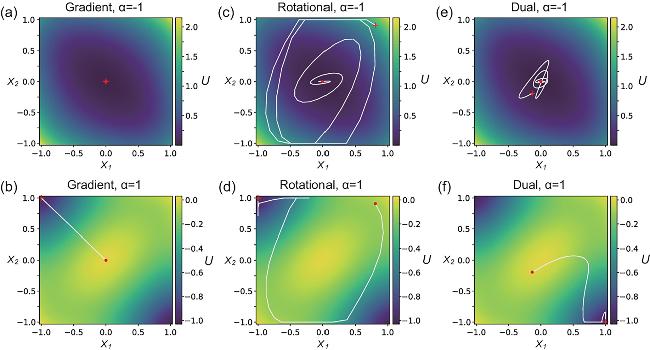
Figure 1. Illustration of the dynamics of gradient, rotational, and dual mean-field dynamics solving a two-spin Ising problem. The spin interactions in this two-spin Ising problem are antiferromagnetic with J11 = J22 = 0 and J12 = J21 = −1. The x1 and x2 represent the positional variables of the two-spin system. The evolved trajectories (white solid lines) for (a) and (b) gradient dynamics, (c) and (d) rotational dynamics, and (e) and (f) dual dynamics in the two-spin position space. In this problem, we linearly increase the bifurcation parameter α with annealing scheme $\alpha ({t}_{k})={\rm{\min }}\{-2+4k/{N}_{\,\rm{step}\,},1\}$, where k = 0, …, Nstep and here we set the total number of iteration steps Nstep = 200. In panels (a), (c) and (e), we show the trajectory segments from start points (red dots) and endpoints (red crosses) corresponding to α increased in interval [−2, 0], and in panels (b), (d) and (f), we show the trajectory segments corresponding to α increased in interval [0, 1]. The heatmaps are the snapshots of the base potential energy function for CIMs in position space at two bifurcation parameter values α = − 1 (panels (a), (c) and (e)) and α = 1 (panels (b), (d) and (f)), showing the different energy landscapes during the evolution. We set the coupling coefficient to c0 = 0.2 for the base potential energy function. For the dual dynamics, the gradient coefficient is g = 0.07, and the rotational coefficient is γ = 1. Additionally, we set the time step Δt = 0.3 for all three dynamics in this problem. |
2.2. Rotational mean-field dynamics of Ising machines and Hamiltonian Monte Carlo
In addition to the gradient dynamics of Ising machines based on equation (2 ), several alternative dynamics have been proposed, including those based on rotational dynamics. For instance, SBM [16, 17, 30] leverages Hamiltonian dynamics, which is a type of rotational dynamics that has been effectively applied within the MCMC framework. As highlighted in the HMC method [22], extending the sampling space into an augmented space can be highly beneficial for sampling efficiency. This approach involves defining new variables ${\boldsymbol{z}}={[{{\boldsymbol{x}}}^{{\rm{T}}},{{\boldsymbol{y}}}^{{\rm{T}}}]}^{{\rm{T}}}\in {{\mathbb{R}}}^{{d}_{x}+{d}_{y}}$, where ${\boldsymbol{x}}\in {{\mathbb{R}}}^{{d}_{x}}$ represents the original state space variables, ${\boldsymbol{y}}\in {{\mathbb{R}}}^{{d}_{y}}$ corresponds to additional auxiliary dimensions, and dx and dy denote their respective dimensions. Simulating the dynamics of the augmented variables z can lead to desirable properties, such as achieving the faster mixing time to sample the uncorrelated samples in the sampling space [23]. Borrowing terminology from statistical physics, we refer to x as the position variables and y as the momentum variables. Accordingly, we denote their joint space as the augmented space (or phase space if x and y have equal dimensions). Note that this notation also accommodates the scenario where y is absent (zero-dimensional). The Hamiltonian function introduced in HMC is defined as 6 ) is rewritten as
$\begin{eqnarray}H({\boldsymbol{z}})=H({\boldsymbol{x}},{\boldsymbol{y}})=U({\boldsymbol{x}},\alpha )+\frac{{{\boldsymbol{y}}}^{{\rm{T}}}{M}^{-1}{\boldsymbol{y}}}{2},\end{eqnarray}$
where the first term in H(z) is also the potential energy U(x, α) associated with the positional variables x, while the second term represents the kinetic energy associated with the momentum variables y scaled by the mass matrix M, because Hamiltonian dynamics is typically used to simulate the physical motion of an object with mass in classical mechanics. The Hamiltonian equations of motion of the rotated dynamics in HMC are written as follows $\begin{eqnarray}\frac{{\rm{d}}{\boldsymbol{y}}}{{\rm{d}}t}=-{{\rm{\nabla }}}_{{\boldsymbol{x}}}\,H({\boldsymbol{x}},{\boldsymbol{y}})=-{{\rm{\nabla }}}_{{\boldsymbol{x}}}\,U({\boldsymbol{x}},\alpha ),\end{eqnarray}$
$\begin{eqnarray}\frac{{\rm{d}}{\boldsymbol{x}}}{{\rm{d}}t}={{\rm{\nabla }}}_{{\boldsymbol{y}}}\,H({\boldsymbol{x}},{\boldsymbol{y}})={M}^{-1}{\boldsymbol{y}},\end{eqnarray}$
when U(x, α) is set to the base potential energy function of CIM and M is set to the identity matrix, where the dimensions dx = dy = N corresponding to N spin variables, equation ( $\begin{eqnarray}\begin{array}{rcl}H({\boldsymbol{x}},{\boldsymbol{y}},\alpha ) & = & \displaystyle \sum _{i}^{N}\left(\frac{1}{4}{x}_{i}^{4}-\frac{\alpha }{2}{x}_{i}^{2}\right)-\frac{{c}_{0}}{2}\displaystyle \sum _{i\lt j}^{N}{J}_{ij}{x}_{i}{x}_{j}\\ & & +\,\frac{1}{2}\displaystyle \sum _{i}^{N}{y}_{i}^{2},\end{array}\end{eqnarray}$
and corresponding Hamiltonian equations of motion are $\begin{eqnarray}\frac{{\rm{d}}{y}_{i}}{{\rm{d}}t}=-{({{\rm{\nabla }}}_{{\boldsymbol{x}}}\,H)}_{i}=-({x}_{i}^{2}-\alpha ){x}_{i}+{c}_{0}\displaystyle \sum _{j}^{N}{J}_{ij}{x}_{j},\end{eqnarray}$
$\begin{eqnarray}\frac{{\rm{d}}{x}_{i}}{{\rm{d}}t}={({{\rm{\nabla }}}_{{\boldsymbol{y}}}\,H)}_{i}={y}_{i},\end{eqnarray}$
which bear some similarities to the rotational dynamics employed in SBM [17], and it has been shown that Hamiltonian rotational dynamics can be beneficial for combinatorial optimization according to their practical performance [16, 17]. Moreover, the widespread use of HMC has proven that it is more efficient to sample and easier to jump out of local optima by using Hamiltonian dynamics than traditional MCMC methods. Similar conclusions can be found in other works that apply transverse forces to the sampling methods [25, 27].Equations (10 ) and (11 ) can be solved using the symplectic Euler method [31]10 ) and (11 ) for the same two-spin Ising problem as in the gradient dynamics, illustrating the behavior of the rotational dynamics. As depicted in the figures, unlike gradient-driven paths in gradient dynamics, trajectories under rotational dynamics circulate within the space even when α is small. Through the augmented space, This circulation enables the system to escape local minima and explore broader areas of the landscape as α increases to discover superior solutions potentially. However, despite this desirable feature, this rotational behavior lacks the mechanisms to determine which minima to converge upon like in gradient dynamics, leading the system to potentially bypass the global minimum, thereby hindering better performance.
$\begin{eqnarray}\begin{array}{rcl}{y}_{i}({t}_{k+1}) & = & {y}_{i}({t}_{k})+\{-[{x}_{i}^{2}({t}_{k})-\alpha ({t}_{k})]{x}_{i}({t}_{k})\\ & & +\,{c}_{0}\displaystyle \sum _{j}^{N}{J}_{ij}{x}_{j}({t}_{k})\}{{\rm{\Delta }}}_{t},\end{array}\end{eqnarray}$
$\begin{eqnarray}\begin{array}{rcl}{x}_{i}({t}_{k+1}) & = & {x}_{i}({t}_{k})+{y}_{i}({t}_{k+1}){{\rm{\Delta }}}_{t},\end{array}\end{eqnarray}$
and like in the gradient dynamics, in the numerical integration, whenever ∣xi(tk)∣ > 1, we set xi(tk) = sign[xi(tk)]. In figures 1(c) and (d), we display the evolution trajectories in the positional space by numerically solving equation (2.3. The dual mean-field dynamics for Ising machines
Building on the existing gradient and rotational dynamics of Ising machines, the proposed dual mean-field dynamics generalizes these approaches by integrating both types of dynamics. This integration facilitates a more comprehensive exploration of the solution space (by rotational dynamics) and enhances convergence performance (by gradient dynamics), leading to the identification of better solutions. Based on the stochastic gradient MCMC [32], we propose the following equations of motion for the dual dynamics with dimensions dx = dy = N in the N-spin Ising problem
$\begin{eqnarray}{\rm{d}}{\boldsymbol{z}}=-[g{\boldsymbol{D}}({\boldsymbol{z}})+\gamma {\boldsymbol{Q}}({\boldsymbol{z}})]{{\rm{\nabla }}}_{{\boldsymbol{z}}}\,H\,{\rm{d}}t,\end{eqnarray}$
where ${\rm{d}}{\boldsymbol{z}}={[{\rm{d}}{{\boldsymbol{x}}}^{{\rm{T}}},{\rm{d}}{{\boldsymbol{y}}}^{{\rm{T}}}]}^{{\rm{T}}}$, ${{\rm{\nabla }}}_{{\boldsymbol{z}}}\,H={[{{\rm{\nabla }}}_{{\boldsymbol{x}}}\,{H}^{{\rm{T}}},{{\rm{\nabla }}}_{{\boldsymbol{y}}}\,{H}^{{\rm{T}}}]}^{{\rm{T}}}$ and D(z) (of dimension 2N × 2N) is called the diffusion matrix that controls the gradient dynamics, and Q(z) (also dimension 2N × 2N) is the skew-symmetric curl matrix that represents the deterministic traversing effects observed in HMC procedures, governing the rotational dynamics. While the matrices D(z) and Q(z) generally depend on z and can be designed to obtain more sophisticated dynamics [32], in this work, we investigate the following constant matrices $\begin{eqnarray}{\boldsymbol{D}}=\left(\begin{array}{cc}{I}_{N} & 0\\ 0 & {I}_{N}\end{array}\right),\quad {\boldsymbol{Q}}=\left(\begin{array}{cc}0 & -{I}_{N}\\ {I}_{N} & 0\end{array}\right).\end{eqnarray}$
Here, IN is the N × N identity matrix. Consequently, we obtain the following equations for the dual dynamics $\begin{eqnarray}{\rm{d}}{\boldsymbol{x}}=-[g{{\rm{\nabla }}}_{{\boldsymbol{x}}}\,{H}-\gamma {{\rm{\nabla }}}_{{\boldsymbol{y}}}\,{H}]\,{\rm{d}}t,\end{eqnarray}$
$\begin{eqnarray}{\rm{d}}{\boldsymbol{y}}=-[\gamma {{\rm{\nabla }}}_{{\boldsymbol{x}}}\,{H}+g{{\rm{\nabla }}}_{{\boldsymbol{y}}}\,{H}]\,{\rm{d}}t.\end{eqnarray}$
Notably, when g = 1 and γ = 0, dual dynamics reduces to gradient dynamics, and when g = 0 and γ = 1, dual dynamics reduces to rotational dynamics. The dynamics in equation (14 ) provide a clear interpretation and correspond to the general scheme of MCMC [32]. Physically, the gradient force drives the spin configuration toward lower energy states, whereas the transverse (rotational) force moves the configuration along paths that preserve the energy level. By carefully tuning and balancing the parameters g and γ, we can optimize performance by combining the two dynamics. For the dual dynamics, we also consider the Hamiltonian H defined in equation (10 ). Thus, equations (17 ) and (18 ) can be solved using the following integration method 18 ) and (19 ) for the same two-spin Ising problem discussed in previous dynamics. The evolution of trajectories under dual dynamics is shown in figures 1(e) and (f). These figures illustrate the behavior of the dual mean-field dynamics, where the trajectories exhibit characteristics of both gradient and rotational dynamics. This dual nature enables thorough exploration of the solution space while effectively converging toward neighboring minima, leading to improved performance.
$\begin{eqnarray}\begin{array}{rcl}{x}_{i}({t}_{k+1}) & = & {x}_{i}({t}_{k})+\left\{\Space{0ex}{2.5ex}{0ex}\Space{0ex}{3.5ex}{0ex}-g\left[{x}_{i}^{2}({t}_{k})-\alpha ({t}_{k})\right]{x}_{i}({t}_{k})\right.\\ & & \left.+\,{c}_{0}g\displaystyle \sum _{j}^{N}{J}_{{ij}}{x}_{j}({t}_{k})+\gamma {y}_{i}({t}_{k})\right\}{{\rm{\Delta }}}_{t},\end{array}\end{eqnarray}$
$\begin{eqnarray}\begin{array}{rcl}{y}_{i}({t}_{k+1}) & = & {y}_{i}({t}_{k})+\left\{\Space{0ex}{3.5ex}{0ex}\Space{0ex}{3.5ex}{0ex}-\gamma \left[{x}_{i}^{2}({t}_{k})-\alpha ({t}_{k})\right]{x}_{i}({t}_{k})\right.\\ & & \left.+\,{c}_{0}\gamma \displaystyle \sum _{j}^{N}{J}_{{ij}}{x}_{j}({t}_{k})-g{y}_{i}({t}_{k})\right\}{{\rm{\Delta }}}_{t},\end{array}\end{eqnarray}$
and in the numerical integration, whenever ∣xi(tk)∣ > 1, we set xi(tk) = sign[xi(tk)]. We numerically solve equations (3. Numerical experiments
3.1. Experiments on Sherrington–Kirkpatrick spin glass model
To assess the effectiveness of the dual dynamics, we apply it to the SK spin glass model [33] to determine its ground state. The SK model serves as a theoretical framework for studying spin glasses and is defined on fully-connected graphs with edge weights drawn from a Gaussian distribution with zero mean and variance of 1/N. This model facilitates the examination of complex optimization landscapes, making it a crucial tool for testing optimization strategies.
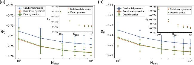
We compared the performance of three dynamics approaches on two generated instances of the SK model, with N = 5000 and N = 10 000 spins. Each dynamics was subjected to the same annealing scheme while varying the total iteration steps Nstep to evaluate the ability to find low-energy states. The outcomes are illustrated in figure 2 (see appendix for experimental parameter settings). The results show that dual and rotational dynamics consistently and significantly outperform gradient dynamics for both N = 5000 and N = 10 000. Additionally, while the average performance difference between dual and rotational dynamics is minimal, dual dynamics consistently achieves lower energy states compared to rotational dynamics as Nstep increases (see the insets in figures 2(a) and (b)). This suggests that dual dynamics enhance the probability of finding superior solutions by effectively incorporating the benefits of gradient dynamics into rotational dynamics.
Figure 2. Comparison of performance between gradient, rotational, and dual dynamics in solving the Sherrington–Kirpatrick (SK) spin glass model. The results of the energy per spin e0 versus total iteration steps Nstep for solving two randomly generated SK model instance with (a) N = 5000 nodes and (b) N = 10 000 nodes. The annealing scheme through all experiments is $\alpha ({t}_{k})={\rm{\min }}\{-2+4k/{N}_{\,\rm{step}\,},1\}$, where k = 0, …, Nstep. We have conducted 10 000 trials for each dynamics in each instance. The solid lines in each figure are the mean values, and the error bars indicate the maximum and minimum values among the trials. The insets indicate the minimum values found by rotational and dual dynamics among the trials. We employed adaptive adjustment for all parameters to ensure optimal results for each dynamics (see |
3.2. Experiments in benchmarking the maximum-cut problem
Next, we test the three dynamics on the maximum-cut (MaxCut) problem [16, 17]. The MaxCut problem is NP-hard and is a fundamental optimization challenge in graph theory and combinatorial optimization, serving as a standard benchmark for evaluating algorithm performance. It focuses on an undirected graph G = (V, E), where the aim is to partition the vertex set V into two disjoint subsets such that the number of edges between these subsets is maximized. In the context of a weighted graph, the objective shifts to maximizing the sum of the weights of these interconnecting edges. The task is to determine this optimal partition, thereby maximizing the ‘cut size' or the total weight of edges between the two groups.
We evaluated the performance of three dynamic approaches on the MaxCut problem using the G-set benchmarking dataset [17, 34]. This dataset includes a variety of graph instances from G1 to G81, ranging from 800 to 20 000 nodes, and includes three types of graphs: random, planar, and toroidal. These instances vary in edge counts and edge weight types. Our experiments focused on larger graphs from the G-set, specifically those containing between 3000 and 10 000 nodes, to assess the effectiveness of the three dynamic approaches in handling large-scale problems. The results are presented in table 1 (with experimental parameter settings detailed in appendix ). For comparison, we also report the best-known results retrieved from H. Goto et al [17] for the MaxCut problem on these graphs.
Table 1. Performance of three dynamics solving the MaxCut benchmarking problems. We present the results of solving relatively large graph instances in the G-set benchmark with a number of nodes ranging from 3000 to 10 000. We only show the best cut values obtained by the three dynamics. The best results are marked in bold. We also report the best-known results retrieved from H. Goto et al [17] for the MaxCut problem on these graphs. We employed adaptive adjustment for all parameters to ensure optimal results for each dynamics (see |
| Instance | Number of | Number of edges | Edge weight type | Graph type | Gradient | Rotational | Dual | Best known |
|---|---|---|---|---|---|---|---|---|
| G48 | 3000 | 6000 | +1, −1 | toroidal | 6000 | 6000 | 6000 | 6000 |
| G49 | 3000 | 6000 | +1, −1 | toroidal | 6000 | 6000 | 6000 | 6000 |
| G50 | 3000 | 6000 | +1, −1 | toroidal | 5880 | 5880 | 5880 | 5880 |
| G55 | 5000 | 12 498 | +1 | random | 10 229 | 10 230 | 10 262 | 10 299 |
| G56 | 5000 | 12 498 | +1, −1 | random | 3969 | 3973 | 3976 | 4017 |
| G57 | 5000 | 10 000 | +1, −1 | toroidal | 3450 | 3462 | 3468 | 3494 |
| G58 | 5000 | 29 570 | +1 | planar | 19 121 | 19 135 | 19 157 | 19 293 |
| G59 | 5000 | 29 570 | +1, −1 | planar | 5986 | 5950 | 5995 | 6087 |
| G60 | 7000 | 17 148 | +1 | random | 14 106 | 14 110 | 14 119 | 14 190 |
| G61 | 7000 | 17 148 | +1, −1 | random | 5704 | 5716 | 5717 | 5798 |
| G62 | 7000 | 14 000 | +1, −1 | toroidal | 4808 | 4828 | 4828 | 4870 |
| G63 | 7000 | 41 459 | +1 | planar | 26 820 | 26 825 | 26 828 | 27 045 |
| G64 | 7000 | 41 459 | +1, −1 | planar | 8592 | 8541 | 8668 | 8751 |
| G65 | 8000 | 16 000 | +1, −1 | toroidal | 5488 | 5508 | 5512 | 5562 |
| G66 | 9000 | 18 000 | +1, −1 | toroidal | 6252 | 6272 | 6282 | 6364 |
| G67 | 10 000 | 20 000 | +1, −1 | toroidal | 6864 | 6882 | 6888 | 6950 |
The results consistently show that both dual dynamics and rotational dynamics outperform gradient dynamics across all tested graphs. Furthermore, dual dynamics demonstrate superior performance over rotational dynamics, achieving better cut values and highlighting the effectiveness of the dual dynamics approach. However, it is worth noting that since our focus in this work is on the base potential energy function introduced in CIMs, the performance varies depending on the graph size. For smaller graph instances (e.g. G48), all three dynamics based on the base potential energy function achieve the best-known results. However, for larger graph instances, the results indicate that the base potential energy function falls short of achieving the best-known solutions, even when dual dynamics is applied. This suggests that, to obtain better solutions for larger graphs, a more carefully designed potential energy function and advanced numerical techniques, such as the discretization trick introduced in [17], are necessary.
4. Conclusion and discussion
In this work, we introduced dual mean-field dynamics, a novel approach for solving combinatorial optimization problems by combining gradient and rotational dynamics within Ising machines. This integration balances the strengths of gradient-driven convergence and rotational exploration, enabling efficient navigation of complex energy landscapes and improving the trade-off between escaping local minima and reaching high-quality solutions. Numerical experiments on the SK spin glass model and the MaxCut problem show that dual dynamics consistently outperform methods using only gradient or rotational dynamics. Specifically, for large instances up to 10 000 spins, dual dynamics achieved lower energy states in the SK model and superior cut values in the MaxCut benchmarks, indicating its scalability and robustness. These results highlight the potential of hybrid dynamical systems in advancing combinatorial optimization. The success of dual dynamics lies in combining gradient guidance towards local minima and rotational exploration of the configuration space, akin to Hamiltonian Monte Carlo's momentum-driven sampling. This dual mechanism helps avoid stagnation in gradient-only methods and aimless wandering in rotational-only approaches. Our findings align with studies on transverse forces in MCMC methods, where violating detailed balance accelerates relaxation without altering stationary distributions, and extend these principles to zero-temperature optimization in deterministic settings.
Despite these advancements, several open questions remain. First, this study focuses solely on the base potential energy function for CIMs. Investigating dual dynamics on other potential energy and Hamiltonian functions is necessary to evaluate its generality. Second, while our experiments used synthetic and benchmark instances, real-world applications, such as logistics or drug discovery, may present additional constraints (e.g. sparse connectivity or heterogeneous couplings) that could challenge the current formulation. These scenarios require careful study within optimization contexts.