


1. Introduction
In his seminal 1939 paper, Rossby examined the relationship between fluctuations in atmospheric zonal circulation intensity and shifts in semi-permanent centers of action. This work introduced the concept of planetary waves (later termed Rossby waves) and established the theoretical foundation for modern Rossby waves studies [1]. Rossby waves are an important type of wave phenomenon in atmospheric and oceanic dynamics, widely used in the study of weather, climate, and ocean circulation. As a result, the theoretical investigation of Rossby waves has become the focus of attention for many scholars worldwide. Scholars [2–4] opened up new avenues of research into Rossby wave theory via mathematical modeling. Matsuno developed an atmospheric wave model for the equatorial region based on the beta-plane approximation and shallow water equations, revealing the core dynamical mechanisms of tropical atmospheric dynamics, analytically derived three types of wave modes in the equatorial region: equatorial Rossby waves, equatorial Kelvin waves, and mixed Rossby-gravity waves [2]. It laid the foundation for later scholars to develop more sophisticated shallow water models, such as Helfrich [5], Grimshaw [6] and Boyd [7]. Hoskins et al analyzed the propagation pathways and energy transport of Rossby waves using the potential vorticity equation [3], laying the groundwork for subsequent researchers to incorporate generalized β-effects, sheared background flows, topography, dissipation, external heat reservoir, stratification effects, and the full Coriolis force [8, 9].
More recently, the QG-PV equation has been a cornerstone of geophysical fluid dynamics, enabling the study of large-scale atmospheric and oceanic flows through scale-invariant analysis. Over the past decade, research has focused on theoretical refinements [10–13], computational innovations [14, 15], and applications to climate dynamics and turbulence[10-14,16]. For instance, Grotjahn et al (2024) proposed a method to generate linearly stable, three-dimensionally localized structures by combining neutral eigenmodes derived from the QG-PV tendency equation [10]. Kuo (2024) developed novel three-dimensional planetary-scale stationary solutions for the nonlinear QG-PV equation, revealing energy dispersion patterns aligned with observed atmospheric and oceanic flows [13]. A 2023 study by Zhao et al used the quasi-geostrophic potential vorticity model to derive a forced Korteweg-de Vries (KdV) equation incorporating the effect of specific topography, which models nonlinear long waves and solitary eddies [16]. The dimensionless QG-PV equation has been instrumental in diagnosing extreme weather and oceanographic phenomena.
Due to the limitations of traditional linear models in describing Rossby wave complexity and the realistic challenges posed by topography and boundary conditions, advanced nonlinear approaches are essential for accurately simulating their dynamics. The Gardner–Morikawa transform is a specific application of the multiple-scale analysis, primarily used to address nonlinear wave problems [17–20]. For instance, by introducing a scaled coordinate system and accounting for Coriolis effects, the authors reduced the original magnetohydrodynamic equations to a modified KdV equation with additional dispersion terms [20]. Therefore, this paper will start from the dimensionless QG-PV equation incorporating external sources and apply a multiple scale expansion method combined with weakly linear perturbation method to derive the mathematical model of Boussinesq equations with external sources, aiming to describe the evolution and development of nonlinear Rossby wave amplitudes.
While numerical methods are essential for solving many complex differential equations, the pursuit of exact solutions remains a cornerstone of scientific and engineering research. They provide fundamental understanding, validate numerical methods, enable practical calculations, and advance mathematical theory. The derivation of exact solutions for partial differential equations remains a pivotal research endeavor in mathematical sciences [21–25]. Therefore, this paper derives analytical solutions for the model equations, specifically including soliton solutions [26–29] and Wronskian solutions [30, 31], to elucidate the influence of external sources on Rossby waves and provide theoretical foundations for interpreting related phenomena in the atmosphere and oceans, while offering insights for marine physics, atmospheric dynamics, meteorological phenomena, and weather prediction. The remainder of this paper is organized as follows: section 2 focuses on the derivation of the nonlinear Boussinesq model equation with external forcing, starting from the dimensionless QG-PV equation and incorporating relevant boundary conditions. We then proceed to find the Wronskian solution and a soliton-like solution of the resulting model equation. Section 2.1 concludes the paper with a summary of the findings.
2. Model and method
2.1. Governing equation and boundary condition
The dimensionless QG-PV equation with external sources is
$\begin{eqnarray}\left(\frac{\partial }{\partial t}+\frac{\partial \psi }{\partial x}\frac{\partial }{\partial y}-\frac{\partial \psi }{\partial y}\frac{\partial }{\partial x}\right)[{{\rm{\nabla }}}^{2}\psi +\beta (y)y]=Q,\end{eqnarray}$
based on the assumption of the generalized β-plane approximation, f = f0 + β(y)y [1], where the function β(y) is nonlinear. The function ψ = ψ(x, y, t) in the equation above denotes the total stream, the function Q = Q(x, y, t) denotes external sources.The boundary condition is
$\begin{eqnarray}\frac{\partial \psi }{\partial x}=0,y=0,1.\end{eqnarray}$
2.2. The externally forced nonlinear Boussinesq equation
Let the total stream function
$\begin{eqnarray}\psi (x,y,t)=-{\int }_{0}^{y}[s(y)-{v}_{0}+\varepsilon \alpha ]{\rm{d}}y+p(x,y,t),\end{eqnarray}$
where s(y) denotes shear effect, v0 is a constant which denotes the phase velocity of nonlinear wave, ϵ is a small parameter (ϵ ≪ 1), α is a constant, whose order of magnitude is 1, and p(x, y, t) is disturbing flow.Let 3 ) into equations (1 ) and (2 ), the equations are converted to 5 ) can be simplified into the following form, 6 ) and (7 ) can be expressed as 9 ), (10 ), we get a set of equations,
$\begin{eqnarray}Q(x,y,t)={Q}_{1}(x,t).\end{eqnarray}$
And substitute it and equation ( $\begin{eqnarray}\begin{array}{l}\frac{\partial }{\partial t}{{\rm{\nabla }}}^{2}\,p+\frac{\partial p}{\partial x}\left[-{s}^{{\prime\prime} }(y)+\frac{\partial }{\partial y}{{\rm{\nabla }}}^{2}\,p\right]\\ \,-\,\left[-s(y)+{v}_{0}-\varepsilon \alpha +\frac{\partial p}{\partial y}\right]\frac{\partial }{\partial x}{{\rm{\nabla }}}^{2}\,p\\ \,+\,\frac{\partial p}{\partial x}\frac{\partial \beta (y)y}{\partial y}={Q}_{1}(x,t),\end{array}\end{eqnarray}$
$\begin{eqnarray}\frac{\partial p}{\partial x}=0,y=0,1,\end{eqnarray}$
where equation ( $\begin{eqnarray}\begin{array}{l}\displaystyle \frac{\partial }{\partial t}{\nabla }^{2}\,p+[s(y)-{v}_{0}+\varepsilon \alpha ]\displaystyle \frac{\partial }{\partial x}{\nabla }^{2}\,p\\ \,+\,\left[\displaystyle \frac{d\beta (y)y}{dy}-{s}{^{\prime\prime} }(y)\right]\displaystyle \frac{\partial p}{\partial x}\\ \,+\,\left(\displaystyle \frac{\partial p}{\partial x}\displaystyle \frac{\partial }{\partial y}-\displaystyle \frac{\partial p}{\partial y}\displaystyle \frac{\partial }{\partial x}\right){\nabla }^{2}\,p={Q}_{1}(x,t).\end{array}\end{eqnarray}$
Apply the Gardner–Morikawa transform, $\begin{eqnarray}X={\varepsilon }^{\frac{1}{2}}x,T=\varepsilon t,\end{eqnarray}$
the equations ( $\begin{eqnarray}\frac{\partial p}{\partial X}=0,y=0,1,\end{eqnarray}$
$\begin{eqnarray}\begin{array}{l}\varepsilon \frac{\partial }{\partial T}\left(\varepsilon \frac{{\partial }^{2}}{\partial {X}^{2}}+\frac{{\partial }^{2}}{\partial {Y}^{2}}\right)p+[s(y)-{v}_{0}+\varepsilon \alpha ]\\ \,{\times \,\varepsilon }^{\frac{1}{2}}\frac{\partial }{\partial X}\left(\varepsilon \frac{{\partial }^{2}}{\partial {X}^{2}}+\frac{{\partial }^{2}}{\partial {Y}^{2}}\right)p+l(y){\varepsilon }^{\frac{1}{2}}\frac{\partial p}{\partial X}\\ \,+\left({\varepsilon }^{\frac{1}{2}}\frac{\partial p}{\partial X}\frac{\partial }{\partial y}-{\varepsilon }^{\frac{1}{2}}\frac{\partial p}{\partial y}\frac{\partial }{\partial X}\right)\left(\varepsilon \frac{{\partial }^{2}}{\partial {X}^{2}}+\frac{{\partial }^{2}}{\partial {Y}^{2}}\right)p={Q}_{1}(x,t),\end{array}\end{eqnarray}$
where $\begin{eqnarray}l(y)=\beta (y)+y{\beta }^{{\prime} }(y)-{s}^{{\prime\prime} }(y),{Q}_{1}(x,t)={\varepsilon }^{\frac{5}{2}}{Q}_{2}(x,t).\end{eqnarray}$
Now, let $\begin{eqnarray}\begin{array}{l}p(X,y,T)=\varepsilon {p}_{0}(X,y,T)+{\varepsilon }^{\frac{3}{2}}{p}_{1}(X,y,T)\\ \,\,+\,{\varepsilon }^{2}{p}_{2}(X,y,T)\,+\cdots ,\end{array}\end{eqnarray}$
and substitute it in the equations ( $\begin{eqnarray}O(\varepsilon ):\left\{\begin{array}{l}(s-{v}_{0})\frac{\partial }{\partial X}\left(\frac{{\partial }^{2}{p}_{0}}{\partial {y}^{2}}\right)+l(y)\frac{\partial {p}_{0}}{\partial X}=0\quad \\ \frac{\partial {p}_{0}}{\partial X}=0,y=0,1,\end{array}\right.\end{eqnarray}$
$\begin{eqnarray}O({\varepsilon }^{\frac{3}{2}}):\left\{\begin{array}{l}\frac{\partial }{\partial T}\left(\frac{{\partial }^{2}{p}_{0}}{\partial {y}^{2}}\right)+(s-{v}_{0})\frac{\partial }{\partial X}\left(\frac{{\partial }^{2}{p}_{1}}{\partial {y}^{2}}\right)+l(y)\frac{\partial {p}_{1}}{\partial X}=0\quad \\ \frac{\partial {p}_{1}}{\partial X}=0,y=0,1,\end{array}\right.\end{eqnarray}$
$\begin{eqnarray}O({\varepsilon }^{2}):\left\{\begin{array}{l}\frac{\partial }{\partial T}\left(\frac{{\partial }^{2}{p}_{1}}{\partial {y}^{2}}\right)+(s-{v}_{0})\left[\frac{{\partial }^{3}{p}_{0}}{\partial {X}^{3}}+\frac{\partial }{\partial X}\left(\frac{{\partial }^{2}{p}_{2}}{\partial {y}^{2}}\right)\right]\\ +\alpha \frac{\partial }{\partial X}\left(\frac{{\partial }^{2}{p}_{0}}{\partial {y}^{2}}\right)+l(y)\frac{\partial {p}_{2}}{\partial X}+\left(\frac{\partial {p}_{0}}{\partial X}\frac{\partial }{\partial y}-\frac{\partial {p}_{0}}{\partial y}\frac{\partial }{\partial X}\right)\frac{{\partial }^{2}{p}_{0}}{\partial {y}^{2}}={Q}_{2}(X,T),\\ \frac{\partial {p}_{2}}{\partial X}=0,y=0,1.\end{array}\right.\end{eqnarray}$
Suppose the expression p0(X, y, T) = U(X, T)φ0(y) satisfies equation (13 ), then when s − v0 ≠ 0, equation (13 ) is equivalent to 14 ) is equivalent to 15 ) is solvable when meeting the condition 19 ) is the standard Boussinesq equation, and because ${\alpha }_{4}\frac{\partial {Q}_{2}}{\partial X}$ represents external sources, in other words, equation (19 ) is a nonlinear Boussinesq equation with external forcing describing the nonlinear Rossby waves.
$\begin{eqnarray}\left\{\begin{array}{l}\frac{{{\rm{d}}}^{2}{p}_{0}}{{\rm{d}}{y}^{2}}+\frac{l(y)}{s-{v}_{0}}{p}_{0}=0\quad \\ {p}_{0}(0)={p}_{0}(1)=0.\quad \end{array}\right.\end{eqnarray}$
Further, suppose $\frac{\partial {p}_{1}}{\partial X}=\frac{\partial U}{\partial T}{\phi }_{1}(y)$, then equation ( $\begin{eqnarray}\left\{\begin{array}{l}\frac{{{\rm{d}}}^{2}{p}_{1}}{{\rm{d}}{y}^{2}}+\frac{l(y)}{s-{v}_{0}}{p}_{1}=-\frac{1}{s-{v}_{0}}\frac{{{\rm{d}}}^{2}{p}_{0}}{{\rm{d}}{y}^{2}}=\frac{l(y)}{{(s-{v}_{0})}^{2}}{p}_{0}\quad \\ {p}_{1}(0)={p}_{1}(1)=0.\quad \end{array}\right.\end{eqnarray}$
Finally, based on the orthogonality of eigenvalue function, equation ( $\begin{eqnarray}\begin{array}{l}{\displaystyle \int }_{0}^{1}\frac{{p}_{0}}{s-{v}_{0}}\frac{\partial }{\partial X}\left[\frac{\partial }{\partial T}\left(\frac{{\partial }^{2}{p}_{1}}{\partial {y}^{2}}\right)+(s-{v}_{0})\frac{{\partial }^{3}{p}_{0}}{\partial {X}^{3}}\right.\\ \,+\alpha \frac{\partial }{\partial X}\left(\frac{{\partial }^{2}{p}_{0}}{\partial {y}^{2}}\right)\,\,+\left(\frac{\partial {p}_{0}}{\partial X}\frac{\partial }{\partial y}-\frac{\partial {p}_{0}}{\partial y}\frac{\partial }{\partial X}\right)\frac{{\partial }^{2}{p}_{0}}{\partial {y}^{2}}\\ \,\left.-{Q}_{2}(X,T)\Space{0ex}{3ex}{0ex}\right]{\rm{d}}y=0.\end{array}\end{eqnarray}$
Then, we simplify the condition as $\begin{eqnarray}\frac{{\partial }^{2}U}{\partial {T}^{2}}+{\alpha }_{1}\frac{{\partial }^{2}U}{\partial {X}^{2}}+{\alpha }_{2}\frac{{\partial }^{2}{U}^{2}}{\partial {X}^{2}}+{\alpha }_{3}\frac{{\partial }^{4}U}{\partial {X}^{4}}={\alpha }_{4}\frac{\partial {Q}_{2}}{\partial X},\end{eqnarray}$
where $\begin{eqnarray}\begin{array}{rcl}{\alpha }_{1} & = & -\frac{\alpha {\displaystyle \int }_{0}^{1}\frac{{p}_{0}{p}_{0}^{{\prime\prime} }}{s-{v}_{0}}{\rm{d}}y}{{\displaystyle \int }_{0}^{1}\frac{{p}_{0}{p}_{1}^{{\prime\prime} }}{s-{v}_{0}}{\rm{d}}y},{\alpha }_{2}=\frac{\displaystyle \int {\,}_{0}^{1}\frac{{p}_{0}^{3}}{s-{v}_{0}}{\left[\frac{l(y)}{s-{v}_{0}}\right]}^{{\prime} }{\rm{d}}y}{2{\displaystyle \int }_{0}^{1}\frac{{p}_{0}{p}_{1}^{{\prime\prime} }}{s-{v}_{0}}{\rm{d}}y},\\ {\alpha }_{3} & = & -\frac{{\displaystyle \int }_{0}^{1}{p}_{0}^{2}{\rm{d}}y}{{\displaystyle \int }_{0}^{1}\frac{{p}_{0}{p}_{1}^{{\prime\prime} }}{s-{v}_{0}}{\rm{d}}y},{\alpha }_{4}=-\frac{{\displaystyle \int }_{0}^{1}\frac{{p}_{0}}{s-{v}_{0}}{\rm{d}}y}{{\displaystyle \int }_{0}^{1}\frac{{p}_{0}{p}_{1}^{{\prime\prime} }}{s-{v}_{0}}{\rm{d}}y}.\end{array}\end{eqnarray}$
When the parameters α4 is zero, equation (2.3. Solutions to the Boussinesq equation
To explain the effect of external sources on the evolution and development of nonlinear Rossby waves, we obtained the soliton-like and Wronskian solutions to the model equation.
2.3.1. Wronskian solutions
We consider the Wronskian solutions of equation (19 ) in the case where the parameter α4 is zero, that is
$\begin{eqnarray}\frac{{\partial }^{2}U}{\partial {T}^{2}}+{\alpha }_{1}\frac{{\partial }^{2}U}{\partial {X}^{2}}+{\alpha }_{2}\frac{{\partial }^{2}{U}^{2}}{\partial {X}^{2}}+{\alpha }_{3}\frac{{\partial }^{4}U}{\partial {X}^{4}}=0.\end{eqnarray}$
Let $U(X,T)=-\frac{{\alpha }_{1}}{2{\alpha }_{2}}+\frac{{\alpha }_{3}}{{\alpha }_{2}}V(x,\sqrt{{\alpha }_{3}}t)$ in the case of α3 > 0, equation (21 ) is equivalent to 22 ), 22 ), that is 22 ), $({D}_{t}^{2}-{D}_{x}^{4})f\cdot f=0$.
$\begin{eqnarray}{V}_{tt}+{({V}^{2})}_{xx}+{V}_{xxxx}=0,\end{eqnarray}$
let $V=6{({\mathrm{ln}}\,f)}_{xx},$ and substitute it into equation ( $\begin{eqnarray}\begin{array}{l}{V}_{tt}+{({V}^{2})}_{xx}+{V}_{xxxx}\\ \,=\,{\left[6\frac{f{f}_{tt}-{f}_{t}^{2}+f{f}_{xxxx}-4{f}_{x}{f}_{xxx}+3{f}_{xx}^{2}}{{f}^{2}}\right]}_{xx}\\ \,=\,{\left[\frac{3({D}_{t}^{2}+{D}_{x}^{4})f\cdot f}{{f}^{2}}\right]}_{xx}=0,\end{array}\end{eqnarray}$
where D denotes the bilinear operator [32], then we find the bilinear form of equation ( $\begin{eqnarray}({D}_{t}^{2}+{D}_{x}^{4})f\cdot f=0.\end{eqnarray}$
In the case of α3 < 0, we can use the similar transform $U(X,T)=-\frac{{\alpha }_{1}}{2{\alpha }_{2}}+\frac{| {\alpha }_{3}| }{{\alpha }_{2}}V(x,\sqrt{| {\alpha }_{3}| }t)$ and $V=-6{({\mathrm{ln}}\,f)}_{xx},$ get the bilinear form of equation (Theorem 2.3.1 If a set of functions of x and t, φi = φi(x, t), i = 1, 2, ⋯, N, satisfies the linear conditions as follows: 24 ), where $f=| \widehat{N-1}| =W({\phi }_{1},{\phi }_{2},\cdots \,{,}{\phi }_{N-1},{\phi }_{N})$ is the Wronskian [33] which is defined as follows:
$\begin{eqnarray}{\phi }_{i,t}=\pm \sqrt{3}{\phi }_{i,xx};{\phi }_{i,xxx}=\displaystyle \sum _{j=1}^{N}{\lambda }_{ij}(t){\phi }_{i},\end{eqnarray}$
[then $f=| \widehat{N-1}| $ solves equation ( $\begin{eqnarray}| \widehat{N-1}| =\left|\begin{array}{ccclr}{\phi }_{1}^{(0)} & {\phi }_{1}^{(1)} & \cdots \, & {\phi }_{1}^{(N-2)} & {\phi }_{1}^{(N-1)}\\ {\phi }_{2}^{(0)} & {\phi }_{2}^{(1)} & \cdots \, & {\phi }_{2}^{(N-2)} & {\phi }_{2}^{(N-1)}\\ \vdots & \vdots & \ddots & \vdots & \vdots \\ {\phi }_{N}^{(0)} & {\phi }_{N}^{(1)} & \cdots \, & {\phi }_{N}^{(N-2)} & {\phi }_{N}^{(N-1)}\\ \end{array}\right|,\end{eqnarray}$
and ${\phi }_{i}^{(0)}={\phi }_{1},{\phi }_{i}^{(j)}=\frac{{\partial }^{j}{\phi }_{i}}{\partial {x}^{j}},j\geqslant 1,1\leqslant i\leqslant N,$λij(t) are real functions.Proof. Now, we proof the function $f=| \widehat{N-1}| $ satisfy equation (24 ), that is to say f is the Wronskian solution [33] of equation (24 ), and $V=6{({\mathrm{ln}}\,f)}_{xx}$ is the Wronskian solution of equation (22 ).25 ) in the theorem 25 ) we have 24 ), $V=6{({\mathrm{ln}}\,f)}_{xx}$ solves the equation (22 ), furthermore $U(X,T)=-\frac{{\alpha }_{1}}{2{\alpha }_{2}}+\frac{{\alpha }_{3}}{{\alpha }_{2}}V(x,\sqrt{{\alpha }_{3}}t)$ solves the model equation (21 ). This proof is finished.
$\begin{eqnarray}({D}_{x}^{4}+{D}_{t}^{2})f\cdot f=2[f{f}_{xxxx}-4{f}_{x}{f}_{xxx}+3{f}_{xx}^{2}+f{f}_{tt}-{f}_{t}^{2}],\end{eqnarray}$
and we have $\begin{eqnarray}\begin{array}{rcl}f & = & | \widehat{N-1}| ,\\ {f}_{x} & = & | \widehat{N-2},N| ,\\ {f}_{xx} & = & | \widehat{N-2},N+1| +| \widehat{N-3},N-1,N| ,\\ {f}_{xxx} & = & | \widehat{N-2},N+2| +2| \widehat{N-3},\\ & & N-1,N+1| +| \widehat{N-4},N-2,N-1,N| ,\\ {f}_{xxxx} & = & | \widehat{N-2},N+3| +3| \widehat{N-3},\\ & & N-1,N+2| +2| \widehat{N-3},N,N+1| \\ & & +3| \widehat{N-4},N-2,N-1,N+1| +| \widehat{N-5},\\ & & N-3,N-2,N-1,N| ,\end{array}\end{eqnarray}$
and we have the following representation base on the first linear condition of ( $\begin{eqnarray}\begin{array}{rcl}{f}_{t} & = & \pm \sqrt{3}[| \widehat{N-3},N,N-1| +| \widehat{N-2},N+1| ],\\ {f}_{tt} & = & \sqrt{3}[-| \widehat{N-5},N-2,N-3,N-1,N| -| \widehat{N-3},\\ & & N+1,N| -| \widehat{N-3},N-1,N+2| \\ & & +| \widehat{N-4},N-1,N-2,N+1| +| \widehat{N-3},\\ & & N,N+1| +| \widehat{N-2},N+3| ]\end{array},\end{eqnarray}$
then we have $\begin{eqnarray}\begin{array}{rcl}f{f}_{tt}+f{f}_{xxxx} & = & f({f}_{tt}+{f}_{xxxx})=| \widehat{N-1}| [4| \widehat{N-2},\\ & & N+3| +8| \widehat{N-3},N,N+1| \\ & & -4| \widehat{N-5},N-2,N-3,N-1,N| ]\\ & = & 4| \widehat{N-1}| [| \widehat{N-2},N+3| -| \widehat{N-5},\\ & & N-2,N-3,N-1,N| ]\\ & & +8| \widehat{N-1}| | \widehat{N-3},N,N+1| \end{array}\end{eqnarray}$
$\begin{eqnarray}\begin{array}{rcl}-{f}_{t}^{2}+3{f}_{xx}^{2} & = & -3{[| \widehat{N-3},N,N-1| +| \widehat{N-2},N+1| ]}^{2}\\ & & +3{[| \widehat{N-2},N+1| +| \widehat{N-3},N-1,N| ]}^{2}\\ & = & -12| \widehat{N-2},N+1| | \widehat{N-3},N,N-1| \\ & = & 12| \widehat{N-2},N+1| | \widehat{N-3},N-1,N| \end{array}\end{eqnarray}$
$\begin{eqnarray}\begin{array}{l}-4{f}_{x}{f}_{xxx}=-4| \widehat{N-2},N| [| \widehat{N-2},\\ \,\,N+2| +2| \widehat{N-3},N-1,N+1| \\ \,\,+| \widehat{N-4},N-2,N-1,N| ]\\ \,=-8| \widehat{N-2},N| | \widehat{N-3},N-1,N+1| \\ \,\,-4| \widehat{N-2},N| [| \widehat{N-2},N+2| \\ \,\,+| \widehat{N-4},N-2,N-1,N| ],\end{array}\end{eqnarray}$
then apply the second linear condition of ( $\begin{eqnarray}\begin{array}{l}| \widehat{N-2},N+3| -| \widehat{N-5},N-2,N-3,N-1,N| \\ \,-| \widehat{N-3},N,N+1| \\ \,=\displaystyle \sum _{i}^{N}{\lambda }_{ii}(t)| \widehat{N-2},N| ,\\ | \widehat{N-2},N+2| +| \widehat{N-3},N-1,N+1| \\ \,+| \widehat{N-4},N-2,N-1,N| \\ \,=\displaystyle \sum _{i}^{N}{\lambda }_{ii}(t)| \widehat{N-1}| .\end{array}\end{eqnarray}$
Now, the bilinear equation is converted to the expression as follows: $\begin{eqnarray}\begin{array}{l}({D}_{t}^{2}+{D}_{x}^{4})f\cdot f=2[f{f}_{tt}-{f}_{t}^{2}+f{f}_{xxxx}-4{f}_{x}{f}_{xxx}+3{f}_{xx}^{2}]\\ \,=24[| \widehat{N-1}| | \widehat{N-3},N,N+1| +| \widehat{N-2},\\ \,N+1| | \widehat{N-3},N-1,N| \\ \,-| \widehat{N-2},N| | \widehat{N-3},N-1,N+1| ],\end{array}\end{eqnarray}$
Actually, set $A=| \widehat{N-3}| $, a = N − 2, b = N − 1, c = N, d = N + 1, then $\begin{eqnarray}\begin{array}{l}({D}_{t}^{2}+{D}_{x}^{4})f\cdot f=24[| A,a,b| | A,c,d| \\ \,+| A,a,d| | A,b,c| -| A,a,c| | A,b,d| ]=0.\end{array}\end{eqnarray}$
This implies that $f=| \widehat{N-1}| $ solves the equation (We can construct Wronskian solutions as the method in [33], and give a rational Wronskian solution of order k − 1 by the steps in [34],
$\begin{eqnarray}\begin{array}{rcl}f & = & W({\psi }_{0},{\psi }_{1},\cdots \,{,}{\psi }_{k-1}),\\ V & = & 6{\partial }_{x}^{2}{\mathrm{ln}}\,W({\psi }_{0},{\psi }_{1},\cdots \,{,}{\psi }_{k-1}),\\ U(X,T) & = & -\frac{{\alpha }_{1}}{2{\alpha }_{2}}+\frac{| {\alpha }_{3}| }{{\alpha }_{2}}V(x,\sqrt{| {\alpha }_{3}| }t).\end{array}\end{eqnarray}$
We can provide a general zero-order Wronskian solution U(X, T) = $-\frac{{\alpha }_{1}}{2{\alpha }_{2}}-$ $\frac{| {\alpha }_{3}| }{{\alpha }_{2}}\frac{12({X}^{2}+2\sqrt{3| {\alpha }_{3}| }T)}{{({X}^{2}-2\sqrt{3| {\alpha }_{3}| }T)}^{2}}$, and a first-order Wronskian solution $U(X,T)=-\frac{{\alpha }_{1}}{2{\alpha }_{2}}-\frac{| {\alpha }_{3}| }{{\alpha }_{2}}\frac{24({X}^{6}-2\sqrt{3| {\alpha }_{3}| }{X}^{4}T+60{\alpha }_{3}{X}^{2}{T}^{2}-24| {\alpha }_{3}| \sqrt{3| {\alpha }_{3}| }{T}^{3})}{{({X}^{4}-4\sqrt{3| {\alpha }_{3}| }{X}^{2}T-12| {\alpha }_{3}| {T}^{2})}^{2}}$, and present their corresponding figures, as shown in figure 1.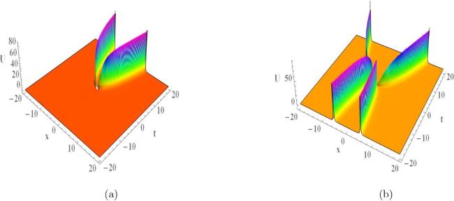
Figure 1. Two general zero-order and first-order Wronskian solutions for equation ( |
2.3.2. Soliton-like solutions
We offer the soliton-like solution by Jacobi elliptic function rational expansion method [35] for equation (19 ) in the case of α4 = 0, that is 21 ) and its corresponding figures are shown in figure 2, where c is phase velocity, c2 = −α1 + α3k2 and k is linear wave number in radial direction.
$\begin{eqnarray}U(X,T)=-\frac{5{\alpha }_{3}{k}^{2}}{2{\alpha }_{2}}+\frac{6{\alpha }_{3}{k}^{2}}{{\alpha }_{2}}{\rm{s}}{\rm{e}}{\rm{c}}{{\rm{h}}}^{2}[k(X-cT)].\end{eqnarray}$
It solves the equation (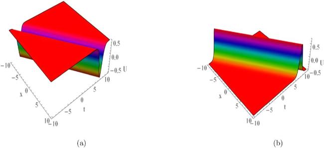
Figure 2. The soliton-like solution of equation ( |
Since equation (21 ) is a special case of equation (19 ), we will now provide the soliton-like solution to equation (19 ) by modified Jacobi elliptic function method [36].
For the sake of investigating the effect of the external sources on Rossby waves and simplifying the calculation, we assume 38 ), (39 ) into the model equation equation (19 ),
$\begin{eqnarray}{\alpha }_{4}\frac{\partial {Q}_{2}}{\partial X}=R(T).\end{eqnarray}$
Let $\begin{eqnarray}U(X,T)=W(X,T)+\tau (T),\end{eqnarray}$
and substitute equations ( $\begin{eqnarray}\begin{array}{l}\frac{{\partial }^{2}W}{\partial {T}^{2}}+({\alpha }_{1}+2{\alpha }_{2}\tau (T))\frac{{\partial }^{2}W}{\partial {X}^{2}}\\ \,+{\alpha }_{2}\frac{{\partial }^{2}({W}^{2})}{\partial {X}^{2}}+{\alpha }_{3}\frac{{\partial }^{4}W}{\partial {X}^{4}}=0,\end{array}\end{eqnarray}$
where $\tau (T)={\int }_{0}^{T}({\int }_{0}^{s}R(t){\rm{d}}t){\rm{d}}w$.Assuming equation (40 ), the Boussinesq equation with variable coefficients, has the following forms of solution, 40 ), the value of n is 2, then 40 ), we can calculate that K(t) is a constant. If K(T) = k, then the following expressions hold, 19 ), that is
$\begin{eqnarray}W(X,T)=\displaystyle \sum _{j=0}^{n}{\omega }_{i}(T)s{n}^{j}[K(T)(X-C(T))].\end{eqnarray}$
Based on equation ( $\begin{eqnarray}\begin{array}{rcl}W(X,T) & = & {\omega }_{0}(T)+{\omega }_{1}(T)sn[K(T)(X-C(T))]\\ & & +{\omega }_{2}(T)s{n}^{2}[K(T)(X-C(T))].\end{array}\end{eqnarray}$
Substitute it into equation ( $\begin{eqnarray}\begin{array}{rcl}{C}^{{\prime} }(T) & = & k({\alpha }_{1}+2{\alpha }_{2}\tau (T)),\\ {\omega }_{0}(T) & = & -\frac{{({\alpha }_{1}+2{\alpha }_{2}\tau (T))}^{2}{k}^{2}+{\alpha }_{1}+2{\alpha }_{2}\tau (T)}{2{\alpha }_{2}},\\ {\omega }_{1}(T) & = & 0,{\omega }_{2}(T)=-\frac{2{\alpha }_{3}{m}^{2}{k}^{2}}{3{\alpha }_{2}}.\end{array}\end{eqnarray}$
Then the following expression can solve the model equation, $\begin{eqnarray}\begin{array}{rcl}U(X,T) & = & -\frac{{({\alpha }_{1}+2{\alpha }_{2}\tau (T))}^{2}{k}^{2}+{\alpha }_{1}+2{\alpha }_{2}\tau (T)}{2{\alpha }_{2}}\\ & & -\frac{2{\alpha }_{3}{m}^{2}{k}^{2}}{3{\alpha }_{2}}s{n}^{2}[k(X-C(T))]+\tau (T),\end{array}\end{eqnarray}$
when m → 1, cn[k(X − C(T))] → sech[k(X − C(T))], we can get the soliton-like solution to equation ( $\begin{eqnarray}\begin{array}{rcl}U(X,T) & = & -\frac{{({\alpha }_{1}+2{\alpha }_{2}\tau (T))}^{2}{k}^{2}+{\alpha }_{1}+2{\alpha }_{2}\tau (T)}{2{\alpha }_{2}}\\ & & -\frac{2{\alpha }_{3}{k}^{2}}{3{\alpha }_{2}}+\frac{2{\alpha }_{3}{k}^{2}}{3{\alpha }_{2}}sec{h}^{2}[k(X-C(T))]\\ & & +\tau (T),\end{array}\end{eqnarray}$
and present its corresponding figures, as shown in figure 3.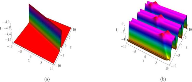
Figure 3. The soliton-like solution of equation ( |
3. Conclusion
We investigate the dimensionless quasi-geostrophic potential vorticity equation with external sources. Using the Gardner–Morikawa transformation and weakly nonlinear perturbation expansion, we derive the nonlinear Boussinesq equation with external sources. We then demonstrate the existence of Wronskian solutions for the model equation when α4 = 0, providing explicit zero-order and first-order Wronskian solutions. Furthermore, employing a modified Jacobi elliptic function method, we obtain soliton-like solutions for the model equation both when α4 = 0 and when α4 ≠ 0.
Since all solutions contain the coefficient of the nonlinear term, α2, it can be inferred that the generalized β-plane approximation and shear flow are significant factors in inducing nonlinear Rossby waves. Furthermore, the expression for the soliton-like solution to the model equation includes τ(T), indicating that external sources also play a role in influencing Rossby wave behavior.