


1. Introduction
Partial differential equations (PDEs) play a crucial role in science, as they reveal the mathematical principles underlying physical systems that are widely used in engineering and technology. In a great deal of existing research on PDEs, it has been found that most of them are difficult to solve analytically. Some traditional methods such as the finite element method [1], the finite difference method [2], and the spectral method [3], have been developed to solve PDEs in a feasible way. However, these numerical methods have several limitations, including mesh dependency, difficulty in designing and weak robustness in higher-order schemes. Due to the advantages of fast computing speed and high accuracy, deep learning based on neural networks has developed rapidly in various fields. In the field of scientific computing, a physically constrained deep learning method known as physics-informed neural networks (PINNs) [4] has recently been proposed for solving forward and inverse problems in differential equations. The central idea of the approach is to add PDEs to the loss function of the neural network using automatic differentiation techniques to minimize the residuals of the PDE while the network approximates the initial and boundary conditions. PINNs introduce the laws of physics behind complex systems and have the advantage of obtaining predictive solutions with relatively little data. In contrast to traditional numerical methods, the PINNs algorithm does not require the discretisation of the spatial and temporal domains. Based on the feasibility of the technique, PINNs have been applied to various types of PDEs, including integral PDEs [5], fractional order PDEs [6], stochastic PDEs [7, 8], etc. Many improved versions of the vanilla PINNs algorithm have emerged, such as gradient-enhanced PINNs (gPINNs) [9], Monte Carlo physically informed neural networks (MC-PINNs) [10], the ensemble physics-informed neural network (E-PINN) [11], the hp-variational PINNs (hp-VPINNs) [12] and so on.
Nonlinear integrable systems are an important branch of mathematical physics and are of great significance for the description of many wave phenomena in nonlinear science. Due to their special mathematical structure, they can be solved by rigorous analytical methods, such as the inverse scattering method, the Hirota bilinear method, the Darboux transform and the Bäcklund transform [13–17]. The analytical methods outlined above can generate extensive training datasets, enabling the PINNs algorithm to effectively solve various nonlinear integrable equations, including the nonlinear Schrödinger (NLS) equations [18], derivative NLS (dNLS) equations [19], Camassa–Holm (CH)-like equations [20–23], and Chen–Lee–Liu equation [24]. In particular, the integrable PINN algorithm has been recently developed involving the convolutional-recurrent network for solving the integrable nonlinear lattice equations and Darboux transformation-based LPNN for generating novel localized wave solutions [25–27]. In these data-driven experiments, PINNs demonstrated strong capabilities both in accurately predicting different types of nonlinear wave solutions, such as soliton, periodic, breather and rogue waves, and in correctly identifying the underlying equation parameters from the known solutions [18–30].
In the field of nonlinear integrable systems, Ablowitz and Musslimani [31] have recently constructed a parity-time (${ \mathcal P }{ \mathcal T }$)-symmetric NLS equation 4 ) describes the solution of the Manakov system under the special initial condition v(x, 0) = u*(x, 0). In this case, the negative time solution u(x, t) of equation (4 ) gives the v(x, t) solution of the Manakov system at positive time through v(x, t) = u*(x, −t). In the same way, [34] has constructed the nonlocal NLS equation of reverse-space and reverse-space-time types and their multi-component generalizations. By employing Hirota’s bilinear method and the Kadomtsev–Petviashvili hierarchy reduction, two types of multiple bright soliton solutions with an even number of solitons were presented for equation (4 ) in the focusing case [35].
$\begin{eqnarray}{\rm{i}}{q}_{t}(x,t)+{q}_{xx}(x,t)+2\sigma {q}^{2}(x,t){q}^{* }(-x,t)=0,\end{eqnarray}$
with the sign of nonlinearity σ = ±1, the asterisk * represents a complex conjugation. This nonlocal equation possesses a fundamental Lax pair formulation and an infinite number of conservation laws, and a number of exact solutions have been obtained by using the traditional techniques adapted to local scenarios [32, 33]. Starting from the well-known integrable Manakov system $\begin{eqnarray}{\rm{i}}{u}_{t}+{u}_{xx}+2\sigma ({\left|u\right|}^{2}+{\left|v\right|}^{2})u=0,\end{eqnarray}$
$\begin{eqnarray}{\rm{i}}{v}_{t}+{v}_{xx}+2\sigma ({\left|u\right|}^{2}+{\left|v\right|}^{2})v=0,\end{eqnarray}$
Yang has introduced a nonlocal reverse-time NLS equation [34] $\begin{eqnarray}\begin{array}{rcl}{\rm{i}}{u}_{t}(x,t) & + & {u}_{xx}(x,t)+2\sigma [{\left|u(x,t)\right|}^{2}\\ & + & {\left|u(x,-t)\right|}^{2}]u(x,t)=0,\end{array}\end{eqnarray}$
by imposing the constraint v(x, t) = u*(x, − t). In the physical background, this reverse-time NLS equation (In addition to the applications on local integrable models, the PINNs algorithm and its enhanced versions have demonstrated remarkable efficiency in solving both forward and inverse problems for nonlocal systems, such as the nonlocal Hirota equation [36], the nonlocal mKdV equation [37], the nonlocal NLS equation of reverse-space type [38], and the NLS equation with PT symmetric potential [39]. In these data-driven examples, it has been found that model training accuracy and computational efficiency are significantly compromised in local regions with sharp gradients for the complicated nonlinear wave solutions. To address this problem, the sample points characterized by large gradients can be detected through gradient calculation and then integrated into the training dataset of neural network. By incorporating these sample points as prior knowledge into PINNs, a hybrid training paradigm has been established to enhance the capability to capture complex physical phenomena [40–44]. In this paper, we employ the PINNs algorithm to perform the data-driven experiments for learning the bright soliton solutions and identifying the unknown parameters in the nonlocal reverse-time NLS equation. In comparison with the PINN models for local coupled NLS systems [29, 30], we construct a relatively simple neural network for the nonlocal reverse-time NLS equation which corresponds to a special class of coupled NLS system. By introducing the nonlocal connection between two components, the numbers of physical constraints from governing equations and objective optimizations can be reduced for the real neural network. Based on the PINNs algorithm, we conduct accurate simulations of two-soliton and four-soliton solutions including linear solitary wave and periodic wave, and present comparative analyses of relative and absolute errors between predicted and exact solutions. More specifically, we use the conventional PINNs framework to train linear solitary wave solutions, while an enhanced sampling strategy that incorporates a priori knowledge of local sharp features is implemented to simulate periodic wave solutions. For the parameter identification, the nonlinear parameters in the nonlocal NLS equation are accurately recognized from noisy and non-noisy exact solutions.
The paper is structured as follows: in section 2 , we introduce the PINNs algorithm for solving the nonlocal NLS equations of reverse-time type. In section 3 , we show the results of numerical experiments for two-soliton and four-soliton solutions and present the comparative analyses of relative and absolute errors. In section 4 , we discuss the problem of identifying parameters in the integrable nonlocal NLS equation and perform comparative experiments from known exact solutions under different noises. Conclusions and discussions are provided in the final section.
2. The PINNs model of the nonlocal reverse-time NLS equation
This section introduces the PINNs model for the nonlocal NLS equation of reverse-time type (4 ). More precisely, the nonlocal NLS equation with initial and Dirichlet boundary condition is expressed by the following form: 5 ) corresponds to the focusing case in equation (4 ) with σ = 1. Define u(x, t) = p(x, t) + iq(x, t), where p(x, t) and q(x, t) are real functions with respect to x and t, representing the real and imaginary parts of u(x, t) respectively, equation (5 ) is divided to two real-valued equations. Then, we can design the real-valued PINNs models fp(x, t) and fq(x, t) with two inputs (x, t) and two outputs $[\hat{p}(x,t),\hat{q}(x,t)]$ such that $\hat{u}(x,t)=\hat{p}(x,t)+{\rm{i}}\hat{q}(x,t)$ to approximate the complex-valued solutions u(x, t):
$\begin{eqnarray}\left\{\begin{array}{l}{\rm{i}}{u}_{t}(x,t)+{u}_{xx}(x,t)+2[| u(x,t){| }^{2}+| u(x,-t){| }^{2}]u(x,t)=0,\,\,x\in [{x}_{0},{x}_{1}],\,\,t\in [{t}_{0},{t}_{1}],\\ u(x,{t}_{0})={u}_{0}(x),\,\,x\in [{x}_{0},{x}_{1}],\\ u({x}_{0},t)={u}_{1}(t),\,\,u({x}_{1},t)={u}_{2}(t),\,\,t\in [{t}_{0},{t}_{1}],\\ \end{array}\right.\end{eqnarray}$
where ${\rm{i}}=\sqrt{-1}$ and u(x, t) is a complex-valued solution of x and t. Here, x0 and x1 denote the lower and upper boundaries of the space variable x, t0 and t1 represent the initial and terminal times. The function u0(x) is an arbitrary complex-valued function of the space variable x. The nonlinear equation ( $\begin{eqnarray}\begin{array}{rcl}{f}_{p} & := & {\hat{p}}_{t}(x,t)+{\hat{q}}_{xx}(x,t)+2[| \hat{p}(x,t){| }^{2}+| \hat{q}(x,t){| }^{2}\\ & & +| \hat{p}(x,-t){| }^{2}+| \hat{q}(x,-t){| }^{2}]\hat{q}(x,t),\end{array}\end{eqnarray}$
$\begin{eqnarray}\begin{array}{c}{f}_{q}\,:= \,{\hat{q}}_{t}(x,t)+{\hat{p}}_{xx}(x,t)+2[| \hat{p}(x,t){| }^{2}+| \hat{q}(x,t){| }^{2}\\ +\,| \hat{p}(x,-t){| }^{2}+| \hat{q}(x,-t){| }^{2}]\hat{p}(x,t).\end{array}\end{eqnarray}$
According to the PINNs algorithm, we construct a fully connected network which has a depth of D. The network architecture comprises an input layer, a D − 1 hidden layers and an output layer. Specifically, the dth hidden layer consists of Nd neurons. By applying the activation function η, the output of the previous layer serves as the input to the subsequent hidden layer. This forward propagation process can be mathematically formulated as the following transformation: 6 ) and (7 ). The solution $\hat{u}(x,t)$ is obtained by training the networks (6 ) and (7 ), which are embedded into the loss function. It is given by the mean-squared objective function: 5 ), which represents learning to satisfy the network outputs fp and fq. The last term denotes the penalty term that incorporates a priori information in the local sharp region into the network. The initial and boundary value data for the solution u(x, t) are expressed by ${\{{x}_{p}^{i},{t}_{p}^{i},{p}^{i}\}}_{i=1}^{{N}_{{ \mathcal I }{ \mathcal B }}}$ and ${\{{x}_{q}^{i},{t}_{q}^{i},{q}^{i}\}}_{i=1}^{{N}_{{ \mathcal I }{ \mathcal B }}}$. The collocation points for fp(x, t) and fq(x, t) are specified as ${\{{x}_{{f}_{p}}^{j},{t}_{{f}_{p}}^{j}\}}_{j=1}^{{N}_{{ \mathcal F }}}$ and ${\{{x}_{{f}_{q}}^{j},{t}_{{f}_{q}}^{j}\}}_{j=1}^{{N}_{{ \mathcal F }}}$ which are sampled using the classical latin hypercube sampling (LHS) technique [45]. The datasets ${\{{x}_{{p}_{r}}^{i},{t}_{{p}_{r}}^{i},{p}_{r}^{i}\}}_{i=1}^{{N}_{{ \mathcal P }}}$ and ${\{{x}_{{q}_{r}}^{i},{t}_{{q}_{r}}^{i},{q}_{r}^{i}\}}_{i=1}^{{N}_{{ \mathcal P }}}$ represent the prior knowledge obtained within the local sharp region. Additionally, the training errors are measured by the relative L2-norm error:
$\begin{eqnarray}{{\boldsymbol{x}}}^{d}=\eta \left({{\boldsymbol{w}}}^{d}{{\boldsymbol{x}}}^{d-1}+{{\boldsymbol{b}}}^{d}\right),\end{eqnarray}$
where ${{\boldsymbol{w}}}^{d}\in {{\mathbb{R}}}^{{N}_{d}\times {N}_{d-1}}$ are the weight matrix, ${{\boldsymbol{b}}}^{d}\in {{\mathbb{R}}}^{{N}_{d}}$ are the bias vectors, respectively. The neural network optimizes the parameters by continuously updating the weights and biases to minimize fp and fq, ensuring that the real part p(x, t) and the imaginary part q(x, t) satisfy equations ( $\begin{eqnarray}{\rm{Loss}}={W}_{{ \mathcal I }{ \mathcal B }}{{\rm{Loss}}}_{{ \mathcal I }{ \mathcal B }}+{W}_{{ \mathcal F }}{{\rm{Loss}}}_{{ \mathcal F }}+{W}_{{ \mathcal P }}{{\rm{Loss}}}_{{ \mathcal P }},\end{eqnarray}$
where ${W}_{{ \mathcal I }{ \mathcal B }}$, ${W}_{{ \mathcal F }}$ and ${W}_{{ \mathcal P }}$ are the adjustable weights for the residual, the initial-boundary conditions and addition of a priori information, respectively. The terms ${\rm{L}}{\rm{o}}{\rm{s}}{{\rm{s}}}_{{ \mathcal I }{ \mathcal B }}$, ${\rm{L}}{\rm{o}}{\rm{s}}{{\rm{s}}}_{{ \mathcal F }}$ and ${\rm{L}}{\rm{o}}{\rm{s}}{{\rm{s}}}_{{ \mathcal P }}$ are given by $\begin{eqnarray}{{\rm{Loss}}}_{{ \mathcal I }{ \mathcal B }}=\frac{1}{{N}_{{ \mathcal I }{ \mathcal B }}}\displaystyle \sum _{i=1}^{{N}_{{ \mathcal I }{ \mathcal B }}}({\left|\hat{p}({x}_{p}^{i},{t}_{p}^{i})-{p}^{i}\right|}^{2}+{\left|\hat{q}({x}_{q}^{i},{t}_{q}^{i})-{q}^{i}\right|}^{2}),\end{eqnarray}$
$\begin{eqnarray}{{\rm{Loss}}}_{{ \mathcal F }}=\frac{1}{{N}_{{ \mathcal F }}}\displaystyle \sum _{j=1}^{{N}_{{ \mathcal F }}}({\left|{f}_{p}({x}_{{f}_{p}}^{j},{t}_{{f}_{p}}^{j})\right|}^{2}+{\left|{f}_{q}({x}_{{f}_{q}}^{j},{t}_{{f}_{q}}^{j})\right|}^{2}),\end{eqnarray}$
$\begin{eqnarray}{{\rm{Loss}}}_{{ \mathcal P }}=\frac{1}{{N}_{{ \mathcal P }}}\displaystyle \sum _{i=1}^{{N}_{{ \mathcal P }}}({\left|\hat{p}({x}_{{p}_{r}}^{i},{t}_{{p}_{r}}^{i})-{p}_{r}^{i}\right|}^{2}+{\left|\hat{q}({x}_{{q}_{r}}^{i},{t}_{{q}_{r}}^{i})-{q}_{r}^{i}\right|}^{2}),\end{eqnarray}$
where the first item corresponds to the initial-boundary conditions, which attempts to fit the known solution data. The second item is used to penalize the nonlocal NLS equation ( $\begin{eqnarray}{{\rm{Error}}}_{u}=\frac{\sqrt{\displaystyle {\sum }_{i=1}^{N}{\left|{u}_{i}(x,t)-{\hat{u}}_{i}(x,t)\right|}^{2}}}{\sqrt{\displaystyle {\sum }_{i=1}^{N}{\left|{u}_{i}(x,t)\right|}^{2}}},\end{eqnarray}$
where ui(x, t) and ${\hat{u}}_{i}(x,t)$ stand for exact and predicted solution, respectively.In the above PINNs algorithm, we use the Adam optimizer and the limited memory Broyden–Fletcher–Goldfarb–Shanno(L-BFGS) optimizer to minimize the loss function. The Adam optimizer is developed based on the gradient descent algorithm, which has the advantage that the size of the parameter updates does not vary with the scaling of the gradient size. The L-BFGS optimizer is a full-batch gradient-based optimization algorithm based on a quasi-Newton method [46], which is suitable for dealing with high-dimensional and unconstrained optimization problems, especially with non-convex or non-smooth functions. In the data-driven experiments, the weights are initialized using the Xavier initialization, the biases are set to zero, and the activation function is chosen as the hyperbolic tangent (tanh) function. All codes in this article are based on Python 3.9 and Tensorflow 2.7. All numerical examples reported here have been run on a computer with a 4060Ti graphics card, a 12-bit Gen Intel(R) Core(TM) i5-12400F 2.5 GHz CPU, and 32-G memory.
3. Data-driven bright soliton solutions of the nonlocal reverse-time NLS equation
In this section, we will use the PINNs algorithm to learn the bright soliton solutions of the reverse-time nonlocal NLS equation (5 ). Bright soliton solutions for equation (5 ) have been derived by using the bilinear method and the KP hierarchy reduction technique [35]. More specifically, the bright soliton solution is formulated as follows:
$\begin{eqnarray}u=\frac{\,\rm{g}\,}{f},\quad f=\left|\begin{array}{cc}{\boldsymbol{A}} & {\boldsymbol{B}}\\ {\boldsymbol{C}} & {\boldsymbol{D}}\end{array}\right|,\quad \,\rm{g}\,=\left|\begin{array}{ccc}{\boldsymbol{A}} & {\boldsymbol{B}} & {{\boldsymbol{\phi }}}_{1}^{{\rm{T}}}\\ {\boldsymbol{C}} & {\boldsymbol{D}} & {{\boldsymbol{\phi }}}_{2}^{{\rm{T}}}\\ {{\boldsymbol{\psi }}}_{1} & {{\boldsymbol{\psi }}}_{2} & 0\end{array}\right|,\end{eqnarray}$
where A, B, C and D are M × M matrices, and φ1, φ2, ψ1 and ψ2 are M-component row vectors whose elements are defined as $\begin{eqnarray}\begin{array}{rcl}{a}_{ij} & = & \frac{{{\rm{e}}}^{{\xi }_{i}+{\eta }_{j}^{* }}+2({\alpha }_{i,1}{\bar{\alpha }}_{j,1}-{\alpha }_{i,2}{\bar{\alpha }}_{j,2})}{{a}_{i}+{a}_{j}+({c}_{i}-{c}_{j})},\\ {b}_{ij} & = & \frac{{{\rm{e}}}^{{\xi }_{i}+{\xi }_{j}^{* }}+2({\alpha }_{i,1}{\alpha }_{j,1}+{\alpha }_{i,2}{\alpha }_{j,2})}{{a}_{i}+{a}_{j}+({c}_{i}+{c}_{j})},\\ {c}_{ij} & = & \frac{{{\rm{e}}}^{{\eta }_{i}+{\eta }_{j}^{* }}+2({\bar{\alpha }}_{i,1}{\bar{\alpha }}_{j,1}+{\bar{\alpha }}_{i,2}{\bar{\alpha }}_{j,2})}{{a}_{i}+{a}_{j}-({c}_{i}+{c}_{j})},\\ {d}_{ij} & = & \frac{{{\rm{e}}}^{{\eta }_{i}+{\xi }_{j}^{* }}+2({\bar{\alpha }}_{i,1}{\alpha }_{j,1}-{\bar{\alpha }}_{i,2}{\alpha }_{j,2})}{{a}_{i}+{a}_{j}-({c}_{i}-{c}_{j})},\\ {{\boldsymbol{\phi }}}_{1} & = & ({{\rm{e}}}^{{\xi }_{1}},{{\rm{e}}}^{{\xi }_{2}},\cdots \,{,}{{\rm{e}}}^{{\xi }_{M}}),\quad {{\boldsymbol{\phi }}}_{2}=({{\rm{e}}}^{{\eta }_{1}},{{\rm{e}}}^{{\eta }_{2}},\cdots \,{,}{{\rm{e}}}^{{\eta }_{M}}),\\ {{\boldsymbol{\psi }}}_{1} & = & -({\bar{\alpha }}_{1},{\bar{\alpha }}_{2},\cdots \,{,}{\bar{\alpha }}_{M}),\,{{\boldsymbol{\psi }}}_{2}=-({\alpha }_{1}^{* },{\alpha }_{2}^{* },\cdots \,{,}{\alpha }_{M}^{* }),\end{array}\end{eqnarray}$
where αi = αi,1 + iαi,2, ${\bar{\alpha }}_{i}$ = ${\bar{\alpha }}_{i,1}$ + ${\rm{i}}{\bar{\alpha }}_{i,2}$, ξi = (ai + ci)x + ${\rm{i}}{({a}_{i}+{c}_{i})}^{2}t$ + θi,0, ηi = (ai − ci)x + ${\rm{i}}{({a}_{i}-{c}_{i})}^{2}t$ + θi,0. The parameters ${a}_{i},{c}_{i},{\theta }_{i,0},{\alpha }_{i,1},{\alpha }_{i,2},{\bar{\alpha }}_{i,1}$ and ${\bar{\alpha }}_{i,2}$ are arbitrary constants for i = 1, 2, …, M.3.1. The two-soliton solution
3.1.1. The degenerate single soliton solution
Based on the above definition of the solution, we give the degenerate single soliton solution with M = 1 under the selected parameters a1 = 0.25, c1 = 1, α1 = 1 + i and ${\bar{\alpha }}_{1}={\theta }_{1,0}=0$:
$\begin{eqnarray}u=\frac{(5-5{\rm{i}}){{\rm{e}}}^{{x}+\frac{25}{16}{\rm{i}}t}}{2+8{{\rm{e}}}^{\frac{5}{2}x}},\end{eqnarray}$
which is a reduced two-soliton solution.For this simple case, we employ a PINNs architecture with six hidden layers and 40 neurons per hidden layer to approximate the degenerate soliton solution of equation (5 ). The computational domain intervals are selected as [x0, x1] = [−4.0, 3.0] for the spatial variable and [t0, t1] = [−0.5, 0.5] for the temporal variable. The spatial interval x ∈ [−4.0, 3.0] is divided into 800 points, and the temporal domain t ∈ [−0.5, 0.5] is partitioned into 600 points. These discretizations are used to generates the datasets for the discretized initial-boundary value. A training dataset is sampled in the manner: Nb = 500 points are randomly selected from the initial-boundary dataset, and Nf = 10000 collocation points are generated using the LHS technique. The weight parameters ${W}_{{ \mathcal I }{ \mathcal B }}$, ${W}_{{ \mathcal F }}$ and ${W}_{{ \mathcal P }}$ in equation (9 ) are set to 1, 1 and 0, respectively. Through the optimization of all parameters, we successfully approximate the degenerate single soliton solution given by (16 ) numerically. The model achieves a relative L2 error of 6.017e−4 within approximately 130 seconds, and the number of iterations required is 2707. figure 1 presents the density plot, error density plot and three-dimensional plot of the predicted solutions $\hat{u}(x,t)$, as well as the loss curve during the training process, respectively. As shown in figure 1, the PINNs algorithm successfully reconstructs the soliton solution (16 ) for the nonlocal reverse-time NLS equation (4 ).

Figure 1. The data-driven bright degenerate single soliton solution of the nonlocal NLS equation ( |
3.1.2. The nondegenerate two-soliton solution
For the nondegenerate two-soliton solution with linear solitons, we set the parameters as a1 = 0.25, c1 = 1, α1 = 1, ${\bar{\alpha }}_{1}={\rm{i}}$ and θ1,0 = 5:
$\begin{eqnarray}\begin{array}{l}u=\frac{6{\rm{i}}{{\rm{e}}}^{\frac{9{\rm{i}}}{16}t+\frac{7}{4}x+15}-3{\rm{i}}{{\rm{e}}}^{\frac{9{\rm{i}}}{16}t-\frac{3}{4}x+5}+10{{\rm{e}}}^{\frac{25{\rm{i}}}{16}t-\frac{1}{4}x+15}+5{{\rm{e}}}^{\frac{25{\rm{i}}}{16}t+\frac{5}{4}x+5}}{16{{\rm{e}}}^{x+20}+2{{\rm{e}}}^{\frac{5}{2}x+10}+2{{\rm{e}}}^{-\frac{3}{2}x+10}+4}.\end{array}\end{eqnarray}$
In this case, we utilize a PINNs architecture consisting of nine hidden layers and 40 neurons per hidden layer for approximating the exact solution (17 ). The intervals of computational domain [x0, x1] and [t0, t1] are set as [−10.0, 14.0] and [−0.5, 0.5], respectively. The spatial and temporal intervals are discretized 800 and 600 points, as described in section 3.1.1 . This manipulation gives rise to the datasets for the initial-boundary value. The number of randomly selected initial-boundary points is set to Nb = 1000 and the number of collocation points produced by the LHS method is Nf = 20000. In the loss equation (9 ), the weight parameters ${W}_{{ \mathcal I }{ \mathcal B }}$, ${W}_{{ \mathcal F }}$ and ${W}_{{ \mathcal P }}$ are still assigned 1, 1 and 0, respectively. After approximately 397 seconds of computation and 3261 iterations, the predictive solution is obtained with a relative L2 error of 1.533e−3. As illustrated in figure 2, the density plot of the predicted solution and the corresponding absolute error plot are shown in figure 2(a). figures 2(b) and (c) display the three-dimensional nonlinear wave plot and the training loss curve, respectively. This result clearly reveals the nonlinear dynamical behavior of the parallel linear two-soliton described by equation (17 ).
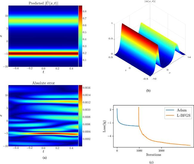
Figure 2. The data-driven parallel two-soliton solution of the nonlocal NLS equation ( |
3.1.3. The two-soliton solution with periodic wave
For the two-soliton solution with periodic wave behavior, we set the free parameters as a1 = 0.25, c1 = 1, α1 = 1, ${\bar{\alpha }}_{1}={\rm{i}}$ and ${\theta }_{1,0}=\frac{1}{5}$:
$\begin{eqnarray}u=\frac{6{\rm{i}}{{\rm{e}}}^{\frac{9{\rm{i}}}{16}t+\frac{7}{4}x+\frac{3}{5}}-3{\rm{i}}{{\rm{e}}}^{\frac{9{\rm{i}}}{16}t-\frac{3}{4}x+\frac{1}{5}}+10{{\rm{e}}}^{\frac{25{\rm{i}}}{16}t-\frac{{x}}{4}+\frac{3}{5}}+5{{\rm{e}}}^{\frac{25{\rm{i}}{t}}{16}+\frac{5}{4}x+\frac{1}{5}}}{16{{\rm{e}}}^{x+\frac{4}{5}}+2{{\rm{e}}}^{\frac{5}{2}x+\frac{2}{5}}+2{{\rm{e}}}^{-\frac{3}{2}x+\frac{2}{5}}+4}.\end{eqnarray}$
In this case, we take the same network architecture and datasets generation approach as described in the previous subsection. The intervals of computational domain [x0, x1] and [t0, t1] are chosen to be [−9.0, 9.0] and [−10.0, 10.0], respectively. The number of initial-boundary points is Nb = 1800 randomly acquired from datasets and the number of collocation points is Nf = 20000 sampled through the LHS approach. The weight parameters ${W}_{{ \mathcal I }{ \mathcal B }}$ and ${W}_{{ \mathcal F }}$ in the loss function remain fixed at 1. When two parallel line solitons approaching each other, they exhibit periodic interactions, resulting in a breathing behavior as demonstrated in figure 3. As can be seen from figure 3(a), unlike the previous line soliton solutions, this periodic wave solution possesses local sharp areas which can affect the training effect. To perform the comparison, we first apply the PINN algorithm without the priori information sample points (${W}_{{ \mathcal P }}=0$) directly to train such solutions. After 26348 iterations, we obtain the training results with the relative L2 error of 6.891e−1. It appears that the original PINN performs poorly for this type of periodic wave solution. To address this problem, we incorporate a priori information within these sharp regions (marked by black forks in the figure) to enhance the accuracy of the training outcomes. Thus, the weight parameter ${W}_{{ \mathcal P }}$ is adjusted to 1, indicating that the priori information sample points are incorporated into the training process. Through 54500 iterations, the network model successfully learned this periodic wave solution, achieving a relative L2 error of 2.383e−3 after approximately 8715 seconds. figure 3(a) shows the predicted solution and the absolute error between the predicted and exact values, demonstrating a high prediction accuracy. figures 3(b) and (c) exhibit the three-dimensional plot that graphically illustrates the collision dynamics between two solitons and the corresponding loss curve during the training process.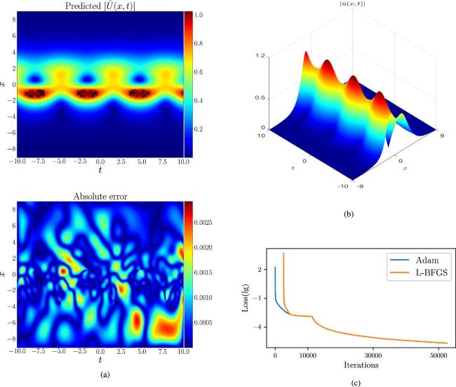
Figure 3. The data-driven bright periodic wave soliton solution of the nonlocal NLS equation ( |
3.2. The four-soliton solution
In this section, we consider the data-driven four-soliton solutions of the nonlocal NLS equation (5 ). To this end, we take M = 2 in equation (14 ) and obtain four-soliton solutions in determinant form: 15 ). The four-soliton solution represents the superposition of two pairs of solitons, and due to the distinct characteristics of each pair, there exists abundant interaction dynamics between two pairs of solitons. For the data-driven experiments, we focus here only on the soliton cases with linear solitary wave and periodic wave.
$\begin{eqnarray}u=\frac{\,\rm{g}\,}{f},\quad f=\left|\begin{array}{cc}{{\boldsymbol{A}}}_{2} & {{\boldsymbol{B}}}_{2}\\ {{\boldsymbol{C}}}_{2} & {{\boldsymbol{D}}}_{2}\end{array}\right|,\quad \,\rm{g}\,=\left|\begin{array}{ccc}{{\boldsymbol{A}}}_{2} & {{\boldsymbol{B}}}_{2} & {{\boldsymbol{\phi }}}_{1}^{(2){\rm{T}}}\\ {{\boldsymbol{C}}}_{2} & {{\boldsymbol{D}}}_{2} & {{\boldsymbol{\phi }}}_{2}^{(2){\rm{T}}}\\ {{\boldsymbol{\psi }}}_{1}^{(2)} & {{\boldsymbol{\psi }}}_{2}^{(2)} & 0\end{array}\right|,\end{eqnarray}$
with $\begin{eqnarray*}\begin{array}{rcl}{{\boldsymbol{A}}}_{2} & = & \left(\begin{array}{cc}{a}_{11} & {a}_{12}\\ {a}_{21} & {a}_{22}\end{array}\right),\ {{\boldsymbol{B}}}_{2}=\left(\begin{array}{cc}{b}_{11} & {b}_{12}\\ {b}_{21} & {b}_{22}\end{array}\right),\\ {{\boldsymbol{C}}}_{2} & = & \left(\begin{array}{cc}{c}_{11} & {c}_{12}\\ {c}_{21} & {c}_{22}\end{array}\right),\ {{\boldsymbol{D}}}_{2}=\left(\begin{array}{cc}{d}_{11} & {d}_{12}\\ {d}_{21} & {d}_{22}\end{array}\right),\\ {{\boldsymbol{\phi }}}_{1}^{(2)} & = & \left({{\rm{e}}}^{{\xi }_{1}},{{\rm{e}}}^{{\xi }_{2}}\right),\ {{\boldsymbol{\phi }}}_{2}^{(2)}=\left({{\rm{e}}}^{{\eta }_{1}},{{\rm{e}}}^{{\eta }_{2}}\right),\ {{\boldsymbol{\psi }}}_{1}^{(2)}=-\left({\bar{\alpha }}_{1},{\bar{\alpha }}_{2}\right),\\ {{\boldsymbol{\psi }}}_{2}^{(2)} & = & -\left({\alpha }_{1}^{* },{\alpha }_{2}^{* }\right),\end{array}\end{eqnarray*}$
where aij, bij, cij, dij, ξi and ηi(i, j = 1, 2) are given by equation (3.2.1. The degenerate three-soliton solution
The degenerate three-soliton solution with linear solitons is a special case of the four-soliton solution, where the parameters in equation (19 ) are chosen as follows: ${\alpha }_{1}={\alpha }_{2}={\bar{\alpha }}_{1}=1$, ${\bar{\alpha }}_{2}=0$, a1 = 1/4, a2 = 2/5, c1 = 2, c2 = 3/2, θ1,0 = −20 and θ2,0 = 4. In order to approximate this exact solution, a PINNs architecture with nine hidden layers and 40 neurons per layer is employed. In the computation domain, the intervals of variables x and t are defined as [−10.0, 15.0] and [−0.3, 0.3], which are subsequently discretized into 800 and 600 grid points to produce the datasets of initial-boundary value. For the sampled dataset, Nb = 1800 points are randomly extracted from the discretized initial-boundary value and Nf = 20000 collocation points are obtained using the LHS method. In the loss function, the weight parameters are taken to be the same as in the case of two linear solitons with ${W}_{{ \mathcal I }{ \mathcal B }}=1$, ${W}_{{ \mathcal F }}=1$ and ${W}_{{ \mathcal P }}=0$. Upon completion of the training, the neural network model achieves a relative L2 error of 9.929e−4 in approximately 8328 seconds, with the number of iterations of 55000. For the training results, the learned solution and the corresponding absolute error plots in figure 4(a) show that the PINNs model is capable of accurately predicting degenerate three-soliton solution with linear solitons in the nonlocal NLS equation (5 ). In figure 4(b), we present the three-dimensional plot of the predicted solution, which depicts three solitons in parallel, consisting of a pair of solitons and a single soliton. The loss curve in figure 4(c) illustrates the convergence behavior of the training process.

Figure 4. The data-driven bright degenerate three-soliton solution of the nonlocal NLS equation ( |
3.2.2. The nondegenerate four-soliton solution
In this subsection, we conduct the data-driven experiment for the nondegenerate four-soliton solution where two pairs of solitons are parallel. For this case, we assign the parameters in equation (19 ) as α1 = α2 = 1, ${\bar{\alpha }}_{1}={\bar{\alpha }}_{2}=0.5$, a1 = 1/4, a2 = 2/5, c1 = 2, c2 = 3/2, θ1,0 = −18 and θ2,0 = 4. The intervals of computational domain [x0, x1] and [t0, t1] are chosen as [−20.0, 15.0] and [−0.3, 0.3], respectively. The datasets of the discretized initial-boundary value are obtained by dividing the spatial and temporal variables into 1000 and 800 points respectively. The neural network architectures, along with the number of initial-boundary points Nb and the number of collocation points Nf, are set identical to those in section 3.2.1 . The weight parameters ${W}_{{ \mathcal I }{ \mathcal B }}$, ${W}_{{ \mathcal F }}$ and ${W}_{{ \mathcal P }}$ in the loss function (9 ) are also set equal to 1, 1 and 0. After 56000 training iterations, the neural network achieved a L2 relative error of 3.517e−3 in approximately 8335s. The training results are illustrated in figure 5, the density plot of the predicted solution and the corresponding absolute error plot are displayed in figure 5(a) visually. figure 5(b) exhibits the three-dimensional plot of four solitons propagating in parallel, which confirms the ability of the established PINNs model to accurately capture the dynamics of the nondegenerate four-soliton solution. figure 5(c) lists the corresponding loss curve during the training process, highlighting the convergence of the network model.
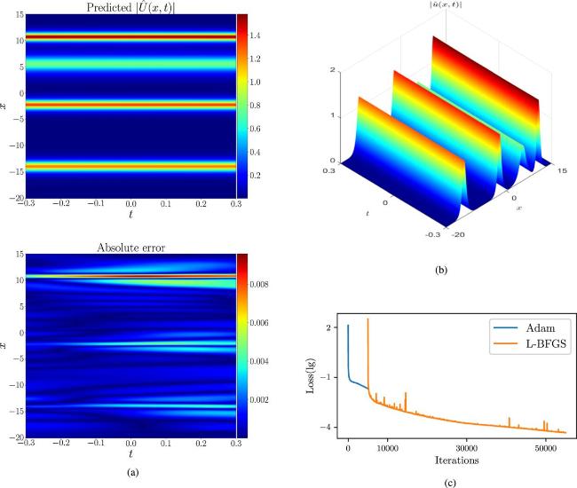
Figure 5. The data-driven parallel four-soliton solution of the nonlocal NLS equation ( |
3.2.3. The four-soliton solution with periodic wave
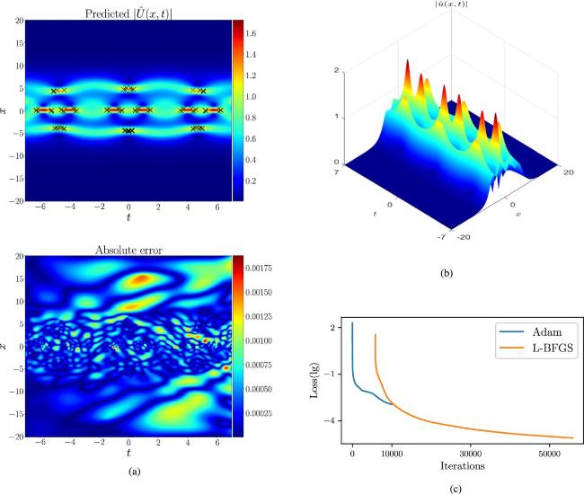
Similar to the periodic wave behavior of two-soliton solutions in section 3.1.3 , the interaction phenomena of two periodic waves will appear in the four-soliton solutions under special parameters. For the purpose of illustration, two examples of data-driven simulations are provided below. In two cases, the parameters in equation (19 ) are chosen to be α1 = ${\alpha }_{2}={\bar{\alpha }}_{1}$ = 1, ${\bar{\alpha }}_{2}=0$, a1 = 1/4, a2 = 2/5, c1 = 3/2, c2 = 1, θ1,0 = 0, θ2,0 = 0 and α1 = α2 = 1, ${\bar{\alpha }}_{1}$ = ${\bar{\alpha }}_{2}=0.5$, a1 = 1/4, a2 = 2/5, c1 = 2, c2 = 3/2, θ1,0 = −20, θ2,0 = 4, respectively. The PINNs architecture and dataset generation method remain unchanged from those outlined in the preceding subsection. For two examples, the computational domain [x0, x1] × [t0, t1] are selected as [−10.0, 7.0] × [−7.0, 7.0] and [−20.0, 20.0] × [−7.0, 7.0], respectively. By splitting the spatial and temporal variables into 1000 and 800 points, respectively, a discretized initial-boundary value dataset is generated. The sampled dataset consisting of the randomly discretized initial-boundary value Nb = 1800 and collocation points Nf = 20000 is obtained in the same manner as in the last subsection. As the periodic wave behavior occurring in two-soliton solutions, the emergence of local sharp regions adversely affects the fitting accuracy of the training. To improve training efficiency, we incorporate prior information from these sharp regions into the training dataset. Hence, the weight parameters of the loss function (9 ) in this case are modified into ${W}_{{ \mathcal I }{ \mathcal B }}={W}_{{ \mathcal F }}={W}_{{ \mathcal P }}=1$. Through optimization of the training parameters to minimize the loss function, we achieve the L2 relative errors of 1.851e−3 and 1.339e−3 for two examples, requiring 55000 and 46228 iterations with training times of 8767 and 7166s, respectively. figures 6 and 7 illustrate the learned four-soliton exhibiting periodic wave behavior, including density plots, absolute error plots and three-dimensional plots as well as the loss curves during the training process. From these numerical results, the complicated wave patterns that indicates the superposed periodic waves can be captured with high accuracy, demonstrating of the robustness of the PINNs model designed for the nonlocal NLS equation (5 ).

Figure 6. The data-driven three-soliton solution with periodic wave for the nonlocal NLS equation ( |
Figure 7. The data-driven three-soliton solution with periodic wave for the nonlocal NLS equation ( |
4. Data-driven parameters discovery of the nonlocal reverse-time NLS equation
In this section, we will study the parameters discovery problem of the nonlocal reverse-time NLS equation (5 ) through the PINNs algorithm, by identifying the parameters of the model from known data. By rewriting the parameters in equation (4 ), it is replaced by the following form 6 ) and (7 ) are modified as follows 5 ), we need to introduce the known information from exact solutions within the domain into the PINNs model to determine the unknown parameters λi. Hence, this gives rise to an additional loss term defined as 9 ) is changed into
$\begin{eqnarray}\begin{array}{l}{\rm{i}}{u}_{t}(x,t)+{u}_{xx}(x,t)+[{\lambda }_{1}{\left|u(x,t)\right|}^{2}\\ \,+{\lambda }_{2}{\left|u(x,-t)\right|}^{2}]u(x,t)=0,\end{array}\end{eqnarray}$
where λi with i = 1, 2 are unknown real coefficients. Therefore, the corresponding real-valued PINNs models ( $\begin{eqnarray}\begin{array}{rcl}{f}_{p} & := & {\hat{p}}_{t}(x,t)+{\hat{q}}_{xx}(x,t)+[{\lambda }_{1}| \hat{p}(x,t){| }^{2}+{\lambda }_{1}| \hat{q}(x,t){| }^{2}\\ & & +{\lambda }_{2}| \hat{p}(x,-t){| }^{2}+{\lambda }_{2}| \hat{q}(x,-t){| }^{2}]\hat{q}(x,t),\end{array}\end{eqnarray}$
$\begin{eqnarray}\begin{array}{rcl}{f}_{q} & := & {\hat{q}}_{t}(x,t)+{\hat{p}}_{xx}(x,t)+[{\lambda }_{1}| \hat{p}(x,t){| }^{2}+{\lambda }_{1}| \hat{q}(x,t){| }^{2}\\ & & +{\lambda }_{2}| \hat{p}(x,-t){| }^{2}+{\lambda }_{2}| \hat{q}(x,-t){| }^{2}]\hat{p}(x,t).\end{array}\end{eqnarray}$
For the parameters discovery problem of equation ( $\begin{eqnarray}\begin{array}{l}{{\rm{Loss}}}_{IN}=\frac{1}{{N}_{IN}}\\ \times \displaystyle \sum _{i=1}^{{N}_{IN}}(| \hat{p}({x}_{IN}^{i},{t}_{IN}^{i})-{p}_{IN}^{i}{| }^{2}+| \hat{q}({x}_{IN}^{i},{t}_{IN}^{i})-{q}_{IN}^{i}{| }^{2}),\end{array}\end{eqnarray}$
where (${x}_{IN}^{i}$, ${t}_{IN}^{i}$) with i = 1, 2, ⋯ , NIN represents a set of random internal points, and $[{p}_{IN}^{i},{q}_{IN}^{i}]$ = $[p({x}_{IN}^{i},{t}_{IN}^{i}),q({x}_{IN}^{i},{t}_{IN}^{i})]$ correspond to the true values of exact solution at these discretized points. Therefore, the loss function ( $\begin{eqnarray}{\rm{Loss}}={W}_{{ \mathcal I }{ \mathcal B }}{{\rm{Loss}}}_{{ \mathcal I }{ \mathcal B }}+{W}_{{ \mathcal F }}{{\rm{Loss}}}_{{ \mathcal F }}+{W}_{IN}{{\rm{Loss}}}_{IN},\end{eqnarray}$
where WIN denotes the weight of the internal information loss term.As demonstrated in the previous section, the PINNs model for solving the forward problem performs higher accuracy and faster convergence for predicting simple soliton solutions. Here we select three types of simpler soliton solutions, including degenerate single soliton, two and four linear soliton solutions as test cases for the inverse problem. For these three cases, we built a network architecture consisting of 9 hidden layers, with 40 neurons per layer and the weights ${W}_{{ \mathcal I }{ \mathcal B }}$, ${W}_{{ \mathcal F }}$ and WIN are all set to 1. In the training process, we first conduct a 5000-step Adam optimization with a default learning rate of 10−3, followed by an L-BFGS optimization with a maximum number of 50000 iterations.
For the data-driven experiments involving three types of solutions, the unknown nonlinear coefficients λi are initialized to λi = 0 and the relative error of these unknown parameters are defined as $\frac{| {\hat{\lambda }}_{i}-{\lambda }_{i}| }{{\lambda }_{i}}$ with i = 1, 2, where ${\hat{\lambda }}_{i}$ and λi represent the predicted and true values, respectively. The computational domains for the degenerate single soliton, parallel linear two- and four-soliton solutions are consistent with those described sections 3.1.1 , 3.1.2 and 3.2.2 , respectively. To generate the discretized datasets of exact solutions including the initial-boundary value and the internal true value, we employ a grid of 800 × 600 points in each spatio-temporal region. For the training datasets, we randomly sample Nb = 1800 initial-boundary points, Nf = 20000 collocation points and NIN = 10000 internal data points by using the LHS method. After optimizing the training parameters in the PINNs model, the learned values of the unknown parameters and their corresponding relative errors are presented in tables 1, 2 and 3 for three types of linear soliton solutions. These results indicate that the PINNs model accurately discovers the unknown parameters, although the relative error increases with the presence of noise. Furthermore, the obtained parameter errors are small regardless of whether the training dataset is affected by noise or not, demonstrating the robustness and effectiveness of the established PINNs model for solving the nonlocal reverse-time NLS equation.
Table 1. The correct nonlocal NLS equation and the identified one with different noise intensity driven by the bright degenerate one-soliton solution ( |
| Nonlocal NLS equation | Item | |
|---|---|---|
| Parameters | Relative errors | |
| Correct | λ1 = 2, λ2 = 2 | λ1: 0%, λ2: 0% |
| Identified (without noise) | λ1 = 1.999653, λ2 = 1.999895 | λ1: 0.01736%, λ2: 0.00538% |
| Identified (with 5% noise) | λ1 = 2.002119, λ2 = 1.997586 | λ1: 0.10593%, λ2: 0.12071% |
| Identified (with 10% noise) | λ1 = 2.002779, λ2 = 1.997199 | λ1: 0.13897%, λ2: 0.14004% |
Table 2. The correct nonlocal NLS equation and the identified one with different noise intensity driven by the parallel two-soliton solution ( |
| Nonlocal NLS equation | Item | |
|---|---|---|
| Parameters | Relative errors | |
| Correct | λ1 = 2, λ2 = 2 | λ1: 0%, λ2: 0% |
| Identified (without noise) | λ1 = 2.006801, λ2 = 1.992423 | λ1: 0.34004%, λ2: 0.37885% |
| Identified (with 5% noise) | λ1 = 2.006532, λ2 = 1.992707 | λ1: 0.32659%, λ2: 0.36466% |
| Identified (with 10% noise) | λ1 = 2.006323, λ2 = 1.992231 | λ1: 0.31613%, λ2: 0.38843% |
Table 3. The correct nonlocal NLS equation and the identified one with different noise intensity driven by the parallel four-soliton solution ( |
| Nonlocal NLS equation | Item | |
|---|---|---|
| Parameters | Relative errors | |
| Correct | λ1 = 2, λ2 = 2 | λ1: 0%, λ2: 0% |
| Identified (without noise) | λ1 = 1.993766, λ2 = 2.005842 | λ1: 0.31171%, λ2: 0.29208% |
| Identified (with 5% noise) | λ1 = 1.976426, λ2 = 2.26032 | λ1: 1.17868%, λ2: 1.30159% |
| Identified (with 10% noise) | λ1 = 1.990758, λ2 = 2.015319 | λ1: 0.46212%, λ2: 0.76593% |
Besides, the internal information points corresponding to actual measured data are crucial to the success of identifying the parameters in inverse problem. Here we conduct the comparison experiments without noise under the different numbers of internal information points and list the result in table 4. It can be seen that the identification accuracy depends on the number of internal information points and the complexity of real solutions.
Table 4. The identified nonlocal NLS equation without noise driven by three types of soliton solutions under different numbers of internal information points. |
| Real solutions | Number of internal information points (NIN) | |||
|---|---|---|---|---|
| 10000 | 5000 | 1000 | 100 | |
| One-soliton ( | λ1: 0.01736% | 0.10909% | 0.12393% | 0.29446% |
| λ2: 0.00538% | 0.05605% | 0.09782% | 0.31192% | |
| | ||||
| Two-soliton ( | λ1: 0.34004% | 0.58463% | 1.24782% | 2.53031% |
| λ2: 0.37885% | 0.66839% | 1.17130% | 2.32259% | |
| | ||||
| Four-soliton ( | λ1: 0.31171% | 1.14817% | 2.30981% | 4.54173% |
| λ2: 0.29208% | 0.96432% | 2.31385% | 4.29937% | |
5. Conclusions and discussions
In this work, we have studied data-driven bright soliton solutions and the parameter identification in the nonlocal NLS equation of reverse-time type through the deep learning framework based on the PINNs algorithm. The training results demonstrate that the established PINNs model with nonlocal constraints is able to accurately simulate two and four-soliton solutions of the nonlocal NLS equations, including the linear solitary wave and the periodic wave. A detailed comparative analysis of the relative and absolute errors between the predicted and exact solutions has been conducted to confirm the performance of the model. More particularly, to pursue the learned solutions with high accuracy, additional prior information is introduced in the training process, particularly in the sharp regions of periodic wave solutions where local variations can significantly impact the training accuracy. In addition, we have also considered the parameter identification problem where the unknown coefficient parameters of nonlinear terms in the nonlocal NLS equations are learned based on the true solutions. The comparative experiments under different noises have been performed to assess the robustness of the proposed PINNs model. However, whether the PINN model can achieve accurate solutions and capture the nonlinear interaction phenomena of different types of nonlinear waves in high-dimensional nonlocal soliton equations deserves further research.