Welcome to visit Communications in Theoretical Physics,
Quantum Physics and Quantum Information

Coherence and entanglement dynamics in Shor’s algorithm

  • Linlin Ye 1 ,
  • Zhaoqi Wu , 1, * ,
  • Shao-Ming Fei 2, 3
Expand
  • 1Department of Mathematics, Nanchang University, Nanchang 330031, China
  • 2School of Mathematical Sciences, Capital Normal University, Beijing 100048, China
  • 3Max Planck Institute for Mathematics in the Sciences, 04103 Leipzig, Germany

Author to whom any correspondence should be addressed.

Received date: 2025-04-16

  Revised date: 2025-07-21

  Accepted date: 2025-07-29

  Online published: 2025-09-12

Supported by

Natural Science Foundation of Jiangxi Province https://doi.org/10.13039/501100004479(20232ACB211003)

National Natural Science Foundation of China https://doi.org/10.13039/501100001809(12075159)

Copyright

© 2025 Institute of Theoretical Physics CAS, Chinese Physical Society and IOP Publishing. All rights, including for text and data mining, AI training, and similar technologies, are reserved.
This article is available under the terms of the IOP-Standard License.

Abstract

Shor’s algorithm outperforms its classical counterpart in efficient prime factorization. We explore the coherence and entanglement dynamics of the evolved states within Shor’s algorithm, showing that the coherence in each step relies on the dimension of register or the order, and discuss the relations between geometric coherence and geometric entanglement. We investigate how unitary operators induce variations in coherence and entanglement, and analyze the variations of coherence and entanglement within the entire algorithm, demonstrating that the overall effect of Shor’s algorithm tends to deplete coherence and produce entanglement. Our research not only deepens the understanding of this algorithm but also provides methodological references for studying resource dynamics in other quantum algorithms.

Cite this article

Linlin Ye , Zhaoqi Wu , Shao-Ming Fei . Coherence and entanglement dynamics in Shor’s algorithm[J]. Communications in Theoretical Physics, 2026 , 78(1) : 015102 . DOI: 10.1088/1572-9494/adf8cc

1. Introduction

Quantum coherence, regarded as a crucial resource, has become a fundamental concept in the field of quantum information processing. It originates from the field of optics and is grounded in the principle of quantum superposition, which is utilized to elucidate the phenomenon of light interference [13]. A foundational framework for quantifying coherence as a resource has been introduced in [4], with an accessible and practical analogous formulation provided in [5]. Based on these frameworks, coherence measures have been presented from the perspective of information [610], such as geometric coherence [11], Tsallis relative α entropy of coherence [12] and l1,p norm of coherence [13]. Quantification of coherence in infinite-dimensional systems has also been considered [14, 15]. On the other hand, coherence manipulation has also attracted much attention and fruitful results have been obtained [1619]. Coherence has found extensive utility across various domains, including biological systems [20, 21], nanoscale physics [22], quantum phase transitions [23] and thermodynamic systems [2428].
The fidelity-based geometric coherence has been established as a full convex coherence monotone [11], offering the advantage of numerical computation through semidefinite programming for finite-dimensional mixed states [29]. Notably, this measure possesses a closed-form expression for single-qubit states, enhancing its practical utility. The lq,p norm [30], which depends solely on the spatial structure of matrices, has been demonstrated to induce a well-defined coherence measure when q = 1 and p ∈ [1, 2] [13], providing a simple closed form incorporating previous norm-induced coherence measures. Regarding entropy-based approaches, Tsallis relative α entropy has been extensively explored as a measure for assessing the purity of a state [31, 32]. Coherence based on it was initially proposed in [33], and later rectified by Zhao and Yu [12] to be a rigorous coherence measure. The Tsallis relative α entropy of coherence and the l1 norm of coherence yield identical ordering for single-qubit pure states [34], suggesting deeper mathematical relationships between seemingly distinct coherence quantifiers.
Entanglement, a unique bond among quantum particles, has been the subject of extensive research over the years. Initially, it was primarily understood as a qualitative aspect of quantum theory, closely related to quantum nonlocality and Bell’s inequality [35, 36]. However, it has also proven to be instrumental in certain contexts like quantum cryptography [37, 38] and is considered as a pivotal resource in quantum computation and information [39, 40]. The geometric entanglement was initially proposed for bipartite pure states [41], and later extended to the multipartite scenario [42] using projectors of varying ranks, which was proven to be an appropriate entanglement quantifier, particularly when dealing with multipartite systems [43]. Furthermore, it is a compelling entanglement measure due to its links with various other measures [44] and the fact that it can be efficiently estimated using quantitative entanglement witnesses, which are suitable for experimental validation [45].
Quantum algorithms can enhance the efficiency of problem-solving on quantum computers [39, 46]. Many quantum algorithms, such as Deutsch–Jozsa algorithm [47, 48], Simon’s algorithm [4951], Grover’s search algorithm [52], Bernstein–Vazirani algorithm [53] and HHL algorithm [54] have been proposed. Shor’s algorithm [55] enables the rapid factorization of large numbers, allowing for the decryption of Rivest–Shamir–Adleman-encrypted communications. The factoring problem can be reduced to a problem of finding the order r, the period of ${x}^{a}{\rm{mod}}\,N$, where N is the number to be factored, and x is an integer coprime to N. Monz [56] utilized a miniature quantum computer comprising five trapped calcium ions to execute a scalable version of Shor’s algorithm. This approach was more efficient than previous implementations and held promise for the design of powerful quantum computers that optimized the use of available resources.
The dynamics of entanglement and coherence within Grover’s algorithm has been the subject of extensive investigation [5765]. Coherence dynamics in Deutsch–Jozsa algorithm, Simon’s quantum algorithm and HHL quantum algorithm have also been investigated in recent years [6569]. Ahnefeld examined a sequential version of Shor’s algorithm that maintains a consistent overall structure, and utilize channel coherence to derive a lower and an upper bound on the success probability of the protocol [70]. Naseri et al [71] investigated the roles of coherence and entanglement as quantum resources in the Bernstein–Vazirani algorithm. In cases where there is no entanglement in the initial and final states of the algorithm, the performance of the algorithm is directly related to the coherence of the initial state. A significant amount of geometric entanglement can prevent the algorithm from achieving optimal performance.
Coherence and entanglement are regarded as the key factors underlying the superior efficiency of quantum algorithms over classical methods in specific computational contexts. By examining the dynamic evolution of quantum resources throughout the algorithms, we can elucidate how quantum superposition and interference facilitate computational speedup, thereby addressing the fundamental question of how quantum resources translate into computational advantages. This analysis not only deepens our theoretical understanding of quantum computation but also provides practical insights for optimizing resource allocation in future quantum algorithmic designs. Our study on quantum coherence and entanglement dynamics in Shor’s algorithm reveals a fundamental relationship between these resources and success probability. The results demonstrate that coherence consumption necessarily precedes probability enhancement, while the algorithm effectively transforms coherence into entanglement critical for quantum speedup.
The remainder of this paper is structured as follows. In section 2, we recall Shor’s algorithm and several coherence and entanglement measures. In section 3, we investigate the coherence and entanglement dynamics in Shor’s algorithm. We explore the variations of coherence and entanglement in Shor’s algorithm in section 4. In section 5, we choose a specific example to illustrate the coherence/entanglement dynamics. Finally, we summarize our results in section 6.

2. Shor’s algorithm and coherence/entanglement quantifiers

In this section, we recall Shor’s algorithm and the quantifiers of coherence and entanglement we use in this paper.

2.1. Shor’s algorithm

The problem of prime factorization is formulated as follows. Given an odd composite positive integer N, the task is to determine its prime factors. It is well known that factoring a composite number N reduces to the order-finding problem. Let N be an integer and x be an integer such that x < N and x is coprime to N. The objective is to find the order r, which is the smallest positive integer satisfying ${x}^{r}=1\,(\mathrm{mod}\,N)$. To deal with this problem the qubit systems comprise a total of n qubits, which are divided into two registers A and B. Register A consists of t qubits with dimension Q = 2t, while register B contains L qubits, where $t=2L+1+\lceil {\mathrm{log}}\,(2+\frac{1}{2\epsilon })\rceil $. Initialize the combined system AB in the state $| 0{\rangle }_{A}^{\otimes t}| 1{\rangle }_{B}$. The main steps of the order-finding algorithm can be summarized as follows [55, 72]:
(i) Apply Hadamard gates ${H}^{\otimes t}=\frac{1}{\sqrt{Q}}{\sum }_{x,y}{(-1)}^{xy}| y\rangle \langle x| $ to the qubits in register A. Then one gets
$\begin{eqnarray}| {\psi }_{1}\rangle =\frac{1}{\sqrt{Q}}\displaystyle \sum _{j=0}^{Q-1}| j\rangle | 1\rangle .\end{eqnarray}$
(ii) Apply the unitary transformation $U={\sum }_{n=0}^{Q-1}| n\rangle \langle n{| }_{A}\otimes {U}_{B}^{n}$ on ∣ψ1⟩, where $U|j\rangle |y\rangle =|j\rangle |{x}^{j}y\,{\rm{mod}}\,N\rangle $ and ${U}_{B}|y{\rangle }_{B}=|xy\,{\rm{mod}}\,N{\rangle }_{B}$. Then one obtains the state
$\begin{eqnarray}| {\psi }_{2}\rangle =\frac{1}{\sqrt{Q}}\displaystyle \sum _{j=0}^{Q-1}| j\rangle | {x}^{j}{\rm{mod}}\,N\rangle .\end{eqnarray}$
Let the eigenvectors of UB be
$\begin{eqnarray}| {u}_{s}\rangle =\frac{1}{\sqrt{r}}\displaystyle \sum _{a=0}^{r-1}{{\rm{e}}}^{-\frac{2\pi {\rm{i}}as}{r}}| {x}^{a}{\rm{mod}}\,N\rangle .\end{eqnarray}$
In particular, one has $\frac{1}{\sqrt{r}}{\sum }_{s=0}^{r-1}|{u}_{s}\rangle =|1\rangle $. The eigenvalues corresponding to ∣us⟩ are ${{\rm{e}}}^{\frac{2\pi {\rm{i}}s}{r}}$. Then we have
$\begin{eqnarray}\begin{array}{rcl}| {\psi }_{2}\rangle & \approx & U\frac{1}{\sqrt{Q}}\displaystyle \sum _{j=0}^{Q-1}| j\rangle | 1\rangle \\ & = & \frac{1}{\sqrt{Q}}\displaystyle \sum _{j=0}^{Q-1}| j\rangle {U}_{B}^{j}\left(\frac{1}{\sqrt{r}}\displaystyle \sum _{s=0}^{r-1}| {u}_{s}\rangle \right)\\ & = & \frac{1}{\sqrt{Qr}}\displaystyle \sum _{s=0}^{r-1}\displaystyle \sum _{j=0}^{Q-1}{{\rm{e}}}^{2\pi {\rm{i}}j\frac{s}{r}}| j\rangle | {u}_{s}\rangle ,\end{array}\end{eqnarray}$
where 0 ≤ sr − 1.
(iii) Applying the inverse Fourier transform F to register A, one has
$\begin{eqnarray}\begin{array}{rcl}| {\psi }_{3}\rangle & = & ({F}^{\dagger }\displaystyle \otimes I)\frac{1}{\sqrt{Qr}}\displaystyle \sum _{s=0}^{r-1}\displaystyle \sum _{j=0}^{Q-1}{{\rm{e}}}^{2\pi {\rm{i}}j\frac{s}{r}}| j\rangle | {u}_{s}\rangle \\ & = & \frac{1}{\sqrt{r}}\displaystyle \sum _{s=0}^{r-1}{F}^{\dagger }\frac{1}{\sqrt{Q}}\displaystyle \sum _{j=0}^{Q-1}{{\rm{e}}}^{2\pi {\rm{i}}j\frac{s}{r}}| j\rangle (I| {u}_{s}\rangle )\\ & = & \frac{1}{\sqrt{r}}\displaystyle \sum _{s=0}^{r-1}| {\psi }_{s}\rangle | {u}_{s}\rangle ,\end{array}\end{eqnarray}$
where $| {\psi }_{s}\rangle ={F}^{\dagger }\frac{1}{\sqrt{Q}}{\sum }_{j=0}^{Q-1}{{\rm{e}}}^{2\pi {\rm{i}}j\frac{s}{r}}| j\rangle =\frac{1}{Q}{\sum }_{j=0}^{Q-1}{\sum }_{k=0}^{Q-1}{{\rm{e}}}^{2\pi {\rm{i}}j(\frac{s}{r}-\frac{k}{Q})}| k\rangle $. We measure the first register to obtain an approximation $\frac{k}{Q}\approx \frac{s}{r}(s\in \{0,1,\ldots ,r-1\})$. ∣k⟩ is a t-bit string that is an estimation of $\frac{s}{r}$ for some s. More specifically, the probability of obtaining measurement outcome k from the first register in step (iii) is given by
$\begin{eqnarray}{p}_{k}=\frac{1}{r}\displaystyle \sum _{s=0}^{r-1}{\left|\frac{1}{Q}\displaystyle \sum _{j=0}^{Q-1}{{\rm{e}}}^{2\pi {\rm{i}}j\Space{0ex}{2.5ex}{0ex}(\frac{s}{r}-\frac{k}{Q}\Space{0ex}{2.5ex}{0ex})}\right|}^{2}.\end{eqnarray}$
Intuitively, the order-finding algorithm randomly selects a value s ∈ {0, 1, …, r − 1} and then returns an approximation to $\frac{s}{r}$ in the form $\frac{k}{Q}$. Finally, by applying the continued fraction algorithm, the order r can be found.

2.2. Measures of coherence and entanglement

The Tsallis relative α entropy is defined as [31, 32]

$\begin{eqnarray}{D}_{\alpha }(\rho \parallel \sigma )=\frac{1}{\alpha -1}\left({f}_{\alpha }(\rho ,\sigma )-1\right),\end{eqnarray}$
where α ∈ (0, 1) ∪ (1, ) and ${f}_{\alpha }(\rho ,\sigma )={\rm{Tr}}({\rho }^{\alpha }{\sigma }^{1-\alpha })$. Note that when α → 1, Dα(ρσ) reduces to ${S}^{{\prime} }(\rho \parallel \sigma )\,={\mathrm{ln}}\,2\cdot S(\rho \parallel \sigma )$, with $S(\rho \parallel \sigma )={\rm{Tr}}(\rho {\mathrm{log}}\,\rho )-{\rm{Tr}}(\rho {\mathrm{log}}\,\sigma )$ representing the standard relative entropy. Here, the logarithm ‘log’ is taken to be base 2.

Let ${\{| i\rangle \}}_{i=1}^{d}$ be an orthonormal basis in a d dimensional Hilbert space H. For α ∈ (0, 1) ∪ (1, 2], the Tsallis relative α-entropy of coherence has been defined by [12]

$\begin{eqnarray}\begin{array}{rcl}{C}_{\alpha }(\rho ) & = & \mathop{\min }\limits_{\sigma \in { \mathcal I }}\frac{1}{\alpha -1}\left({f}_{\alpha }^{\frac{1}{\alpha }}(\rho ,\sigma )-1\right)\\ & = & \frac{1}{\alpha -1}\left[\displaystyle \sum _{i=1}^{d}{\langle i| {\rho }^{\alpha }| i\rangle }^{\frac{1}{\alpha }}-1\right],\end{array}\end{eqnarray}$
and was proven to be a family of bona-fide coherence measures, where ${ \mathcal I }$ denotes the set of incoherent states, which are diagonal matrices in the given basis. Note that when α → 1, Cα(ρ) reduces to ${\mathrm{ln}}\,2\cdot {C}_{r}(\rho )$, where ${C}_{r}(\rho )={\rm{Tr}}(\rho {\mathrm{log}}\,\rho )-{\rm{Tr}}({\rho }_{{\rm{diag}}}{\mathrm{log}}\,{\rho }_{{\rm{diag}}})$ is the relative entropy of coherence [4], with ρdiag denotes the diagonal part of the state ρ. Also, Cα(ρ) reduces to 2Cs(ρ) when $\alpha =\frac{1}{2}$, where ${C}_{s}(\rho )=1-{\sum }_{j=1}^{d}{\langle j| \sqrt{\rho }| j\rangle }^{2}$ is the skew information of coherence [8].

The lq,p norm of a matrix A ∈ Mn is defined as the lq norm of the vector obtained by applying the lp norm to the columns of A, given by [13]

$\begin{eqnarray}{l}_{q,p}(A)={\left(\displaystyle \sum _{j=1}^{n}{l}_{p}{({A}_{j})}^{q}\right)}^{\frac{1}{q}},\end{eqnarray}$
where 1 ≤ p, q, Aj denotes the columns of A, and ${l}_{p}({A}_{j})={\left({\sum }_{i=1}^{n}| {A}_{i,j}{| }^{p}\right)}^{\frac{1}{p}}$, with Ai,j being the entry of the ith row and jth column of matrix A.

Note that lp,p norm is actually the lp norm. The coherence based on lq,p norm is a well-defined coherence measure if and only if q = 1 and p ∈ [1, 2].

The l1,p norm of coherence C1,p of a density operator ρ for p ∈ [1, 2] is defined by [13]

$\begin{eqnarray}\begin{array}{r}\begin{array}{rcl}{C}_{1,p}(\rho ) & = & \mathop{\min }\limits_{\sigma \in { \mathcal I }}{l}_{1,p}(\rho -\sigma )={l}_{1,p}(\rho -{\rho }_{{\rm{diag}}})\\ & = & \displaystyle \sum _{j=1}^{n}{\left(\displaystyle \sum _{i=1}^{n}| {(\rho -{\rho }_{{\rm{diag}}})}_{i,j}{| }^{p}\right)}^{\frac{1}{p}},\end{array}\end{array}\end{eqnarray}$
where ${(\rho -{\rho }_{{\rm{diag}}})}_{i,j}$ is the (i, j)th entry of ρ − ρdiag.

The coherence C1,p introduces a class of coherence measures that hold potential utility and expands the methodological framework for analyzing quantum coherence in multipartite systems. It is worthwhile to note that when p = q = 1, C1,p(ρ) reduces to the l1 norm of coherence ${C}_{{l}_{1}}(\rho )={\sum }_{i\ne j}| {\rho }_{ij}| $ [4].

The fidelity between two quantum states ρ and σ is defined by $F(\rho ,\sigma )={\rm{Tr}}\sqrt{{\rho }^{\frac{1}{2}}\sigma {\rho }^{\frac{1}{2}}}$ [39]. Particularly, when ρ = ∣ψ⟩⟨ψ∣ is a pure state, we have $F(| \psi \rangle ,\sigma )={\rm{Tr}}\sqrt{\langle \psi | \sigma | \psi \rangle }$.

The geometric coherence is defined by [11]

$\begin{eqnarray}{C}_{g}(\rho )=1-{\left[\mathop{\max }\limits_{\delta \in { \mathcal I }}F(\rho ,\delta )\right]}^{2}.\end{eqnarray}$
For a pure state ∣ψ⟩ = ∑iλii⟩, its geometric coherence is given by
$\begin{eqnarray}{C}_{g}(\rho )=1-\mathop{\max }\limits_{i}\{| {\lambda }_{i}{| }^{2}\},\end{eqnarray}$
where ∣λi2 are the diagonal elements of ∣ψ⟩⟨ψ∣.

The geometric entanglement for a state ρ = ∣ψ⟩⟨ψ∣ is defined as the minimum distance to any separable state ∣φ⟩, which corresponds to the maximum overlap between ∣ψ⟩and ∣φ⟩ [41],

$\begin{eqnarray}{E}_{g}(\rho )=1-\mathop{\max }\limits_{| \phi \rangle }| \langle \psi | \phi \rangle {| }^{2},\end{eqnarray}$
where the maximum is taken over all separable states $| \phi \rangle ={\otimes }_{s=1}^{n}| {\phi }_{s}\rangle $, with ∣φs⟩ denoting the single-qubit pure states.

3. Coherence and entanglement dynamics in Shor’s algorithm

In this section, we examine the dynamics of coherence and entanglement in the state resulting from the application of each basic operator within Shor’s algorithm.
Let ρ1 = ∣ψ1⟩⟨ψ1∣ be the density operator of the state ∣ψ1⟩. By employing equations (1), (8), (10) (12) and (13) we have

The l1,p norm of coherence, the Tsallis relative α entropy of coherence, the geometric coherence and the geometric entanglement of the state ρ1 are given by

$\begin{eqnarray}{C}_{1,p}({\rho }_{1})={\left(Q-1\right)}^{\frac{1}{p}},\end{eqnarray}$
$\begin{eqnarray}{C}_{\alpha }({\rho }_{1})=\frac{1}{\alpha -1}\left({Q}^{1-\frac{1}{\alpha }}-1\right),\end{eqnarray}$
$\begin{eqnarray}{C}_{g}({\rho }_{1})=1-\frac{1}{Q},\end{eqnarray}$
and
$\begin{eqnarray}{E}_{g}({\rho }_{1})=0,\end{eqnarray}$
respectively.

According to Theorem 1, the l1,p norm of coherence, the Tsallis relative α entropy of coherence, and the geometric coherence of ρ1 are all dependent on the dimension of register Q, while the entire system represented by ρ1 does not manifest any entanglement. Also, note that

$\begin{eqnarray*}{C}_{g}({\rho }_{1})+{E}_{g}({\rho }_{1})\lt 1.\end{eqnarray*}$

The optimization of the geometric entanglement is achievable for a subset of symmetric separable states ∣ηn, where $| \eta \rangle =\cos \frac{\alpha }{2}| 0\rangle +{{\rm{e}}}^{{\rm{i}}\beta }\sin \frac{\alpha }{2}| 1\rangle $, with α ∈ [0, π], β ∈ [0, 2π] and i the imaginary unit. Since the coefficients of ∣ψ2⟩ are all positive, one sets β = 0. To simplify the analysis, we consider the case where Q = rm with m being a positive integer, which implies that $\unicode{x0230A}\frac{Q-1}{r}\unicode{x0230B}=m-1$. Expressing the index as j = a + br, the state ∣ψ2⟩ can be approximately expressed as $\frac{1}{\sqrt{Q}}{\sum }_{a=0}^{r-1}{\sum }_{b=0}^{m-1}| a+br\rangle | {x}^{a}{\rm{mod}}N\rangle $, where 0 ≤ ar − 1 and 0 ≤ bm − 1. Letting $| {S}_{a}\rangle \,={\sum }_{b=0}^{m-1}| a+br\rangle | {x}^{a}{\rm{mod}}N\rangle $, we can then rewrite ∣ψ2⟩ as
$\begin{eqnarray*}\sqrt{\frac{1}{Q}}\displaystyle \sum _{a=0}^{r-1}| {S}_{a}\rangle .\end{eqnarray*}$
Recall that the Hamming weight of a basis state ∣x⟩ is the number of 1’s in the binary string x ∈ {0, 1}n, and we use ∣x∣ to denote the Hamming weight of ∣x⟩ [58].
Let ρ2 = ∣ψ2⟩⟨ψ2∣ be the density operator of the state ∣ψ2⟩, and the following result then holds.

The Tsallis relative α entropy of coherence, the l1,p norm of coherence and the geometric coherence of the state ρ2 are the same as the ones of ρ1. The geometric entanglement of the state ρ2 is given by

$\begin{eqnarray}\begin{array}{lcl}{E}_{g}({\rho }_{2}) & = & 1-\frac{1}{Q}\\ & & \times \,{\left(\displaystyle \sum _{a=0}^{r-1}\displaystyle \sum _{b=0}^{m-1}{\left(\frac{n-{n}_{a,b}}{n}\right)}^{\frac{n-{n}_{a,b}}{2}}{\left(\frac{{n}_{a,b}}{n}\right)}^{\frac{{n}_{a,b}}{2}}\right)}^{2},\end{array}\end{eqnarray}$
where na,b is the Hamming weight of $| a+br\rangle | {x}^{a}{\rm{mod}}N\rangle (a=0,1,\cdots \,,r-1$ and b = 01,⋯, m − 1).

Direct calculations show that

$\begin{eqnarray*}{C}_{1,p}({\rho }_{1})={C}_{1,p}({\rho }_{2}),\,\,{C}_{\alpha }({\rho }_{1})={C}_{\alpha }({\rho }_{2})\,\,{\rm{and}}\,\,{C}_{g}({\rho }_{2})={C}_{g}({\rho }_{1}).\end{eqnarray*}$
The symmetric n-separable state can be expressed as
$\begin{eqnarray*}|\phi \rangle =|\eta {\rangle }^{\otimes n}=\displaystyle \sum _{x\in {\{0,1\}}^{n}}{\cos }^{n-|x|}\frac{\alpha }{2}{\sin }^{|x|}\frac{\alpha }{2}|x\rangle ,\end{eqnarray*}$
where ∣x∣ represents the Hamming weight of ∣x⟩. According to [57], the overlap between the state ∣ψ2⟩ and the separable state ∣φ⟩ is
$\begin{eqnarray*}\langle {\psi }_{2}| \phi \rangle =\sqrt{\frac{1}{Q}}\displaystyle \sum _{a=0}^{r-1}\left(\displaystyle \sum _{b=0}^{m-1}{\cos }^{n-{n}_{a,b}}\frac{\alpha }{2}{\sin }^{{n}_{a,b}}\frac{\alpha }{2}\right),\end{eqnarray*}$
where na,b is the Hamming weight of $| a+br\rangle | {x}^{a}{\rm{mod}}N\rangle $. Then the maximum overlap between the state ∣ψ2⟩ and the separable state ∣φ⟩ is
$\begin{eqnarray*}\begin{array}{l}\mathop{\max }\limits_{| \phi \rangle }| \langle {\psi }_{2}| \phi \rangle {| }^{2}\\ \quad =\,\mathop{\max }\limits_{\alpha }{\left|\frac{1}{\sqrt{Q}}\displaystyle \sum _{a=0}^{r-1}\displaystyle \sum _{b=0}^{m-1}{\cos }^{n-{n}_{a,b}}\frac{\alpha }{2}{\sin }^{{n}_{a,b}}\frac{\alpha }{2}\right|}^{2}.\end{array}\end{eqnarray*}$
Denote $A(\alpha )={\cos }^{n-{n}_{a,b}}\frac{\alpha }{2}{\sin }^{{n}_{a,b}}\frac{\alpha }{2}$. The maximum of A(α) is
$\begin{eqnarray*}A{(\alpha )}_{\max }={\left(\frac{n-{n}_{a,b}}{n}\right)}^{\frac{n-{n}_{a,b}}{2}}{\left(\frac{{n}_{a,b}}{n}\right)}^{\frac{{n}_{a,b}}{2}}.\end{eqnarray*}$
Therefore, we get
$\begin{eqnarray*}\begin{array}{rcl}\mathop{\max }\limits_{| \phi \rangle }| \langle {\psi }_{2}| \phi \rangle {| }^{2} & = & \frac{1}{Q}\\ & & \times {\left(\displaystyle \sum _{a=0}^{r-1}\displaystyle \sum _{b=0}^{m-1}{\left(\frac{n-{n}_{a,b}}{n}\right)}^{\frac{n-{n}_{a,b}}{2}}{\left(\frac{{n}_{a,b}}{n}\right)}^{\frac{{n}_{a,b}}{2}}\right)}^{2},\end{array}\end{eqnarray*}$
which is attained at $\alpha =2\arccos \sqrt{\frac{n-{n}_{a,b}}{n}}$. From equation (13), we then have
$\begin{eqnarray*}\begin{array}{rcl}{E}_{g}({\rho }_{2}) & = & 1-\frac{1}{Q}\\ & & \times {\left(\displaystyle \sum _{a=0}^{r-1}\displaystyle \sum _{b=0}^{m-1}{\left(\frac{n-{n}_{a,b}}{n}\right)}^{\frac{n-{n}_{a,b}}{2}}{\left(\frac{{n}_{a,b}}{n}\right)}^{\frac{{n}_{a,b}}{2}}\right)}^{2}.\end{array}\end{eqnarray*}$

It can be seen from Theorem 2 that Eg(ρ2) depends on the dimension of register A, the total number of qubits in the system, the Hamming weight of $| a+br\rangle | {x}^{a}{\rm{mod}}N\rangle $and the order r, while both Eg(ρ2) and Cg(ρ2) are less than 1 and dependent on Q. Moreover, we have

$\begin{eqnarray*}{C}_{g}({\rho }_{2})+\frac{1}{\gamma (n,{n}_{a,b})}(1-{E}_{g}({\rho }_{2}))=1,\end{eqnarray*}$
where $\gamma (n,{n}_{a,b})={\left({\sum }_{a=0}^{r-1}{\sum }_{b=0}^{m-1}{\left(\frac{n-{n}_{a,b}}{n}\right)}^{\frac{n-{n}_{a,b}}{2}}{\left(\frac{{n}_{a,b}}{n}\right)}^{\frac{{n}_{a,b}}{2}}\right)}^{2}$ and 0 < γ(nna,b) < Q. It is easy to see that Eg(ρ2) becomes larger if Cg(ρ2) is larger, while Cg(ρ2) > Eg(ρ2) whenγ(nna,b) > 1, Cg(ρ2) < Eg(ρ2) when γ(nna,b) < 1 and Cg(ρ2) = Eg(ρ2) when γ(nna,b) = 1.

For a given s ∈ {0, 1, …, r − 1}, to simplify the analysis, we consider the ideal case in which there exists an integer ks such that $\frac{{k}_{s}}{Q}=\frac{s}{r}$ holds, i.e. ${k}_{s}=\frac{sQ}{r}=sm$. Then the expression for ∣ψs⟩ can be simplified to $| {\psi }_{s}\rangle ={F}^{\dagger }\frac{1}{\sqrt{Q}}{\sum }_{j=0}^{Q-1}{{\rm{e}}}^{2\pi {\rm{i}}j\frac{{k}_{s}}{Q}}| j\rangle =| {k}_{s}\rangle $, and thus ∣ψ3⟩ can be rewritten as
$\begin{eqnarray}\begin{array}{rcl}| {\psi }_{3}\rangle & = & \frac{1}{\sqrt{r}}\displaystyle \sum _{s=0}^{r-1}| {\psi }_{s}\rangle | {u}_{s}\rangle =\frac{1}{\sqrt{r}}\displaystyle \sum _{s=0}^{r-1}| {k}_{s}\rangle | {u}_{s}\rangle \\ & = & \frac{1}{r}\displaystyle \sum _{s,a=0}^{r-1}{{\rm{e}}}^{-\frac{2\pi {\rm{i}}as}{r}}| {k}_{s}\rangle | {x}^{a}{\rm{mod}}\,N\rangle .\end{array}\end{eqnarray}$
Let ρ3 be the density operator of the state ∣ψ3⟩. We have by direct calculation the following theorem.

The l1,p norm of coherence, the Tsallis relative α entropy of coherence, the geometric coherence and the geometric entanglement of the state ρ3 are given by

$\begin{eqnarray}{C}_{1,p}({\rho }_{3})={\left({r}^{2}-1\right)}^{\frac{1}{p}},\end{eqnarray}$
$\begin{eqnarray}{C}_{\alpha }({\rho }_{3})=\frac{1}{\alpha -1}\left(\Space{0ex}{2.5ex}{0ex}{r}^{2\Space{0ex}{2.5ex}{0ex}(1-\frac{1}{\alpha }\Space{0ex}{2.5ex}{0ex})}-1\Space{0ex}{2.5ex}{0ex}\right),\end{eqnarray}$
$\begin{eqnarray}{C}_{g}({\rho }_{3})=1-\frac{1}{{r}^{2}},\end{eqnarray}$
and
$\begin{eqnarray}\begin{array}{l}{E}_{g}({\rho }_{3})=1-\frac{1}{{r}^{2}}\\ \times {\left(\displaystyle \sum _{a,s=0}^{r-1}{{\rm{e}}}^{-\frac{2\pi {\rm{i}}sa}{r}}{\left(\frac{n-{m}_{a,s}}{n}\right)}^{\frac{n-{m}_{a,s}}{2}}{\left(\frac{{m}_{a,s}}{n}\right)}^{\frac{{m}_{a,s}}{2}}\right)}^{2},\end{array}\end{eqnarray}$
respectively, where ma,s is the Hamming weight of $| {k}_{s}\rangle | {x}^{a}{\rm{mod}}N\rangle $(a, s = 0, 1,⋯, r − 1).

By substituting equation (19) into equations (8), (10) and (12), we obtain equations (20), (21) and (22). Rewrite $| {\psi }_{3}\rangle =\frac{1}{r}{\sum }_{a,s=0}^{r-1}{{\rm{e}}}^{-\frac{2\pi {\rm{i}}sa}{r}}| {k}_{s}\rangle | {x}^{a}{\rm{mod}}N\rangle $ as

$\begin{eqnarray*}\frac{1}{r}\displaystyle \sum _{a,s=0}^{r-1}{{\rm{e}}}^{-\frac{2\pi {\rm{i}}sa}{r}}| {W}_{a,s}\rangle ,\end{eqnarray*}$
where $|{W}_{a,s}\rangle =|{k}_{s}\rangle |{x}^{a}{\rm{mod}}N\rangle $. According to [57], the overlap between the separable state ∣φ⟩ and the state ∣ψ3⟩ is
$\begin{eqnarray*}\langle {\psi }_{3}| \phi \rangle =\frac{1}{r}\displaystyle \sum _{a,s=0}^{r-1}{{\rm{e}}}^{-\frac{2\pi {\rm{i}}sa}{r}}{\cos }^{n-{m}_{a,s}}\frac{\alpha }{2}{\sin }^{{m}_{a,s}}\frac{\alpha }{2},\end{eqnarray*}$
where ma,s is the Hamming weight of $| {k}_{s}\rangle | {x}^{a}{\rm{mod}}N\rangle $. Denote $B(\alpha )={\cos }^{n-{m}_{a,s}}\frac{\alpha }{2}$ ${\sin }^{{m}_{a,s}}\frac{\alpha }{2}$. It is verified that when $\alpha =2\arccos \sqrt{\frac{n-{m}_{a,s}}{n}}$, the maximum value of B(α) is
$\begin{eqnarray*}B{(\alpha )}_{\max }={\left(\frac{n-{m}_{a,s}}{n}\right)}^{\frac{n-{m}_{a,s}}{2}}{\left(\frac{{m}_{a,s}}{n}\right)}^{\frac{{m}_{a,s}}{2}}.\end{eqnarray*}$
Then the maximum of the overlap between the separable state ∣φ⟩ and the state ∣ψ3⟩ is
$\begin{eqnarray*}\begin{array}{r}\begin{array}{l}\mathop{\max }\limits_{| \phi \rangle }| \langle {\psi }_{3}| \phi \rangle {| }^{2}\\ =\,\mathop{\max }\limits_{\alpha }{\left|\frac{1}{r}\displaystyle \sum _{a,s=0}^{r-1}{{\rm{e}}}^{-\frac{2\pi {\rm{i}}sa}{r}}{\cos }^{n-{m}_{a,s}}\frac{\alpha }{2}{\sin }^{{m}_{a,s}}\frac{\alpha }{2}\right|}^{2}\\ =\,\frac{1}{{r}^{2}}{\left(\displaystyle \sum _{a,s=0}^{r-1}{{\rm{e}}}^{-\frac{2\pi {\rm{i}}sa}{r}}{\left(\frac{n-{m}_{a,s}}{n}\right)}^{\frac{n-{m}_{a,s}}{2}}{\left(\frac{{m}_{a,s}}{n}\right)}^{\frac{{m}_{a,s}}{2}}\right)}^{2}.\end{array}\end{array}\end{eqnarray*}$
Hence, according to equation (13) we have
$\begin{eqnarray*}\begin{array}{l}{E}_{g}({\rho }_{3})=1-\frac{1}{{r}^{2}}\\ \times {\left(\displaystyle \sum _{a,s=0}^{r-1}{{\rm{e}}}^{-\frac{2\pi {\rm{i}}sa}{r}}{\left(\frac{n-{m}_{a,s}}{n}\right)}^{\frac{n-{m}_{a,s}}{2}}{\left(\frac{{m}_{a,s}}{n}\right)}^{\frac{{m}_{a,s}}{2}}\right)}^{2}.\end{array}\end{eqnarray*}$

Theorem 3 indicates that the l1,p norm of coherence, the Tsallis relative α entropy of coherence and the geometric coherence of the state ρ3 are all determined by the order r, while the geometric entanglement of the state ρ3 depends on the total number of qubits in the system, the Hamming weight of $| {k}_{s}\rangle | {x}^{a}{\rm{mod}}\,N\rangle $and the order r. Note that both Eg(ρ3) and Cg(ρ3) are less than 1 and depend on r. Besides, it holds that

$\begin{eqnarray*}{C}_{g}({\rho }_{3})+\frac{1}{\gamma (n,{m}_{a,s})}(1-{E}_{g}({\rho }_{3}))=1,\end{eqnarray*}$
where $\gamma (n,{m}_{a,s})={\left({\sum }_{a,s=0}^{r-1}{{\rm{e}}}^{-\frac{2\pi {\rm{i}}sa}{r}}{\left(\frac{n-{m}_{a,s}}{n}\right)}^{\frac{n-{m}_{a,s}}{2}}{\left(\frac{{m}_{a,s}}{n}\right)}^{\frac{{m}_{a,s}}{2}}\right)}^{2}$ and 0 < γ(nma,s) < r2. Similarly, Eg(ρ3) becomes larger if Cg(ρ3) is larger, while Cg(ρ3) > Eg(ρ3) when γ(nma,s) > 1, Cg(ρ3) < Eg(ρ3) when γ(nma,s) < 1 and Cg(ρ3) = Eg(ρ3) when γ(nma,s) = 1.

4. Variations of coherence and entanglement in Shor’s algorithm

In this section, we investigate how unitary operators induce variations in coherence and entanglement, and analyze the variations of coherence and entanglement within the entire algorithm.
Following [58] and [61], we define the variation of coherence and entanglement induced by a unitary operator V on a state ∣ψ⟩ to be
$\begin{eqnarray}{\rm{\Delta }}C(V,\rho )\equiv C(V\rho {V}^{\dagger })-C(\rho ),\end{eqnarray}$
and
$\begin{eqnarray}{\rm{\Delta }}E(V,\rho )\equiv E(V\rho {V}^{\dagger })-E(\rho ),\end{eqnarray}$
respectively, and the variation of coherence and entanglement in Shor’s quantum algorithm to be
$\begin{eqnarray}{\rm{\Delta }}C(\rho )\equiv C({\rho }_{3})-C({\rho }_{1}),\end{eqnarray}$
and
$\begin{eqnarray}{\rm{\Delta }}E(\rho )\equiv E({\rho }_{3})-E({\rho }_{1}),\end{eqnarray}$
respectively.
Combining equations (14)–(17), (20)–(23) and Theorem 2, we have

The variations of coherence and entanglement induced by each operator are

$\begin{eqnarray}{\rm{\Delta }}{C}_{1,p}(U,{\rho }_{1})=0,\end{eqnarray}$
$\begin{eqnarray}{\rm{\Delta }}{C}_{1,p}({F}^{\dagger },{\rho }_{2})={\left({r}^{2}-1\right)}^{\frac{1}{p}}-{\left(Q-1\right)}^{\frac{1}{p}},\end{eqnarray}$
$\begin{eqnarray}{\rm{\Delta }}{C}_{\alpha }(U,{\rho }_{1})=0,\end{eqnarray}$
$\begin{eqnarray}{\rm{\Delta }}{C}_{\alpha }({F}^{\dagger },{\rho }_{2})=\frac{1}{\alpha -1}\left[\Space{0ex}{2.5ex}{0ex}{r}^{2\Space{0ex}{2.5ex}{0ex}(1-\frac{1}{\alpha }\Space{0ex}{2.5ex}{0ex})}-{Q}^{1-\frac{1}{\alpha }}\Space{0ex}{2.5ex}{0ex}\right],\end{eqnarray}$
$\begin{eqnarray}{\rm{\Delta }}{C}_{g}(U,{\rho }_{1})=0,\end{eqnarray}$
$\begin{eqnarray}{\rm{\Delta }}{C}_{g}({F}^{\dagger },{\rho }_{2})=\frac{1}{Q}-\frac{1}{{r}^{2}},\end{eqnarray}$
$\begin{eqnarray}\begin{array}{l}{\rm{\Delta }}{E}_{g}(U,{\rho }_{1})=1-\frac{1}{Q}\\ \times \,{\left(\displaystyle \sum _{a=0}^{r-1}\displaystyle \sum _{b=0}^{m-1}{\left(\frac{n-{n}_{a,b}}{n}\right)}^{\frac{n-{n}_{a,b}}{2}}{\left(\frac{{n}_{a,b}}{n}\right)}^{\frac{{n}_{a,b}}{2}}\right)}^{2}\end{array}\end{eqnarray}$
and
$\begin{eqnarray}\begin{array}{r}\begin{array}{l}{\rm{\Delta }}{E}_{g}({F}^{\dagger },{\rho }_{2})\\ \,=\,\frac{1}{Q}{\left(\displaystyle \sum _{a=0}^{r-1}\displaystyle \sum _{b=0}^{m-1}{\left(\frac{n-{n}_{a,b}}{n}\right)}^{\frac{n-{n}_{a,b}}{2}}{\left(\frac{{n}_{a,b}}{n}\right)}^{\frac{{n}_{a,b}}{2}}\right)}^{2}\\ \,-\,\frac{1}{{r}^{2}}{\left(\displaystyle \sum _{a,s=0}^{r-1}{{\rm{e}}}^{-\frac{2\pi {\rm{i}}sa}{r}}{\left(\frac{n-{m}_{a,s}}{n}\right)}^{\frac{n-{m}_{a,s}}{2}}{\left(\frac{{m}_{a,s}}{n}\right)}^{\frac{{m}_{a,s}}{2}}\right)}^{2},\end{array}\end{array}\end{eqnarray}$
respectively.

In Shor’s algorithm, Q represents the dimension of register A and is specifically chosen to satisfy the constraint N2Q < 2N2. Combining this with the fact that rN, we can derive the inequality Qr2. This relationship leads to ΔC1,p(Fρ2) < 0, ΔCα(Fρ2) < 0, ΔCg(Fρ2) < 0 and ΔEg(Uρ1) ≥ 0. Our analysis further reveals a distinct characterization of the operators’ effects within the algorithm. Specifically, while the operator U preserves the coherence of state ρ1, it simultaneously generates entanglement. In contrast, the operator F demonstrably consumes coherence throughout its application. Furthermore, the behavior of F with respect to entanglement exhibits more nuanced properties and demonstrates condition-dependency, suggesting a complex interplay between different quantum resources during computational processes.
Based on equations (26) and (27) and Theorem 4, we obtain the following result immediately.

The variations of coherence and entanglement in Shor’s algorithm are
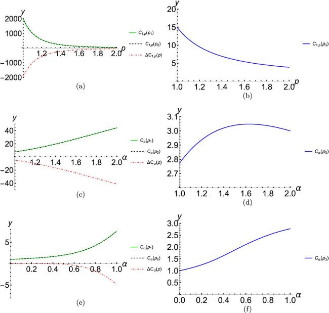
$\begin{eqnarray}{\rm{\Delta }}{C}_{1,p}(\rho )={\left({r}^{2}-1\right)}^{\frac{1}{p}}-{\left(Q-1\right)}^{\frac{1}{p}},\end{eqnarray}$
$\begin{eqnarray}{\rm{\Delta }}{C}_{\alpha }(\rho )=\frac{1}{\alpha -1}\left[\Space{0ex}{2.5ex}{0ex}{r}^{2\Space{0ex}{2.5ex}{0ex}(1-\frac{1}{\alpha }\Space{0ex}{2.5ex}{0ex})}-{Q}^{1-\frac{1}{\alpha }}\Space{0ex}{2.5ex}{0ex}\right],\end{eqnarray}$
$\begin{eqnarray}{\rm{\Delta }}{C}_{g}(\rho )=\frac{1}{Q}-\frac{1}{{r}^{2}}\end{eqnarray}$
and
$\begin{eqnarray}\begin{array}{l}{\rm{\Delta }}{E}_{g}(\rho )=1-\frac{1}{{r}^{2}}\\ \times {\left(\displaystyle \sum _{a,s=0}^{r-1}{{\rm{e}}}^{-\frac{2\pi {\rm{i}}sa}{r}}{\left(\frac{n-{m}_{a,s}}{n}\right)}^{\frac{n-{m}_{a,s}}{2}}{\left(\frac{{m}_{a,s}}{n}\right)}^{\frac{{m}_{a,s}}{2}}\right)}^{2},\end{array}\end{eqnarray}$
respectively.

Combining this with the inequality Qr2, we can derive that ΔC1,p(ρ) < 0, ΔCα(ρ) < 0 and ΔCg(ρ) < 0. Corollary 1 reveals a fundamental resource redistribution in Shor’s algorithm, which indicates that coherence is depleted throughout the computation. In contrast, ΔEg(ρ) > 0 suggests that entanglement is actively generated. This dual behavior reflects a resource conversion process, where coherence is consumed to fuel entanglement production. Such dynamics highlight the interplay between coherence and entanglement as key factors in the algorithm’s efficiency. This provides a critical insight for optimizing quantum algorithms: by strategically managing coherence depletion and entanglement generation, it may be possible to enhance computational efficiency while minimizing resource costs.

5. Example

In this section, we present an example to elucidate the characters of coherence and entanglement in the state after the application of each basic operator within Shor’s algorithm.

Let N = 15 and x = 7 that is coprime to N. The initial quantum state is ∣0⟩t∣1⟩, where the number t of qubits in register A is related to the precision. Here, we set t = 11, which ensures that the probability of error is less than one quarter. The number L of qubits in register B needs to accommodate the binary representation of the integer N, that is, L = 4 and n = 15.

(i) Applying t Hadamard gates to register A yields the state $| {\psi }_{1}\rangle =\frac{1}{\sqrt{{2}^{11}}}{\sum }_{j=0}^{{2}^{11}-1}| j\rangle | 1\rangle $. Let ρ1 = ∣ψ1⟩⟨ψ1∣, from Theorem 1, we have ${C}_{1,p}({\rho }_{1})={\left({2}^{11}-1\right)}^{\frac{1}{p}}$, ${C}_{\alpha }({\rho }_{1})=\frac{1}{\alpha -1}$ $\left({2}^{11(1-\frac{1}{\alpha })}-1\right)$, Cg(ρ1) ≈ 0.9995 and Eg(ρ1) = 0.

(ii) The quantum state resulting from the application of the unitary transformation U is $| {\psi }_{2}\rangle =\frac{1}{\sqrt{{2}^{11}}}{\sum }_{j=0}^{{2}^{11}-1}| j\rangle | {7}^{j}{\rm{mod}}15\rangle $. $| {7}^{j}{\rm{mod}}15\rangle $ takes on one of the four states ∣1⟩, ∣7⟩, ∣4⟩ and ∣13⟩.

Letting ρ2 = ∣ψ2⟩⟨ψ2∣, by Theorem 2, we have C1,p(ρ2) = C1,p(ρ1), Cα(ρ2) = Cα(ρ1), Cg(ρ2) = Cg(ρ1) ≈ 0.9995 and
$\begin{eqnarray*}\begin{array}{rcl}{E}_{g}({\rho }_{2}) & = & 1-\frac{1}{{2}^{11}}\\ & & \times {\left(\displaystyle \sum _{a=0}^{3}\displaystyle \sum _{b=0}^{511}{\left(\frac{15-{n}_{a,b}}{15}\right)}^{\frac{15-{n}_{a,b}}{2}}{\left(\frac{{n}_{a,b}}{15}\right)}^{\frac{{n}_{a,b}}{2}}\right)}^{2}\\ & \approx & 0.8445,\end{array}\end{eqnarray*}$
where na,b is the Hamming weight of $| a+4b\rangle | {7}^{a}{\rm{mod}}15\rangle $. (iii) After applying the inverse Fourier transform F to the register A, from Theorem 3, we can obtain ${C}_{1,p}({\rho }_{3})=1{5}^{\frac{1}{p}}$, ${C}_{\alpha }({\rho }_{3})=\frac{1}{\alpha -1}\left(1{6}^{1-\frac{1}{\alpha }}-1\right)$, Cg(ρ3) = 0.9375 and
$\begin{eqnarray*}\begin{array}{l}{E}_{g}({\rho }_{3})=1-\frac{1}{16}\\ \,\times \,{\left(\displaystyle \sum _{a=0}^{3}\displaystyle \sum _{s=0}^{3}{{\rm{e}}}^{\frac{-2\pi {\rm{i}}sa}{4}}{\left(\frac{15-{m}_{a,s}}{15}\right)}^{\frac{15-{m}_{a,s}}{2}}{\left(\frac{{m}_{a,s}}{15}\right)}^{\frac{{m}_{a,s}}{2}}\right)}^{2}\\ \,\approx \,0.9876,\end{array}\end{eqnarray*}$
where ma,s is the Hamming weight of $| {2}^{9}s\rangle | {7}^{a}{\rm{mod}}15\rangle $.
(iv) The variations of coherence based on the l1,p norm and the Tsallis relative α entropy during the Shor’s algorithm are given by ${\rm{\Delta }}{C}_{1,p}(\rho )=1{5}^{\frac{1}{p}}-{\left({2}^{11}-1\right)}^{\frac{1}{p}}$ and
$\begin{eqnarray*}{\rm{\Delta }}{C}_{\alpha }(\rho )=\frac{1}{\alpha -1}\left[1{6}^{1-\frac{1}{\alpha }}-{2}^{11(1-\frac{1}{\alpha }\Space{0ex}{2.5ex}{0ex})}\right],\end{eqnarray*}$
respectively. Also, we have ΔCg(ρ) = −0.062 and ΔEg(ρ) = 0.9876.
In step (ii), if register B measurement yields ∣4⟩ from $| {7}^{j}{\rm{mod}}15\rangle $, then the state of register A becomes $\sqrt{\frac{4}{{2}^{t}}}[| 2\rangle +| 6\rangle +| 10\rangle +| 14\rangle +\ldots ]$. After applying F, measurement will yield one of four states: ∣0⟩, ∣512⟩, ∣1024⟩ or ∣1536⟩. If ∣1536⟩ is measured, then $\frac{1536}{2048}=\frac{3}{4}$ gives r = 4. Since ${7}^{2}{\rm{mod}}15\ne \pm 1$, we obtain (72 − 1, 15) = 3 and (72 + 1, 15) = 5 as non-trivial factors of N = 15.
For H, U and F operations, coherence based on the l1,p norm decreases with increasing p, while its variation increases. Based on Tsallis relative α entropy, coherence for H and U increases with α, while variation decreases within α ∈ (0, 1) ∪ (1, 2]. F exhibits more complex behavior: when α ∈ (1, 2], coherence peaks at α* ≈ 1.629; when α ∈ (0, 1), coherence consistently increases with α (see figure 1).
Figure 1. Subfigures (a) and (b) ((c), (d), (e) and (f)) are for the case that the coherence based on the l1,p norm (Tsallis relative α entropy). (a), (b) The coherence with respect to H (green), U (black dashed), F (blue) and the variations of coherence based on the l1,p norm (red dot-dashed). (c), (d) The coherence with respect to H (green), U (black dashed), F (blue) and the variations of coherence based on the Tsallis relative α entropy (red dot-dashed), where α ∈ (1, 2]. (e), (f) The coherence with respect to H (green), U (black dashed), F (blue) and the variations of coherence based on the Tsallis relative α entropy (red dot-dashed), where α ∈ (0, 1).

6. Conclusions and discussions

We have investigated how coherence and entanglement impact on the Shor’s algorithm, by calculating how they change during each step of the algorithm. We have studied the variations of coherence and entanglement during Shor’s algorithm and found that, irrespective of the employed coherence quantifier, coherence tends to deplete, while entanglement is generated throughout the process. Furthermore, the behavior of F in Shor’s algorithm can either consume or generate entanglement, depending on the order r, the Hamming weight, and the dimensions of each register.
Entanglement dynamics exhibit scale invariance for large n in Grover’s search algorithm [59], implying that the geometric entanglement does not depend on the number of qubits n and is solely determined by the ratio of iteration k to the total number of iterations. Here we show that the geometric entanglement is not always scale invariant, but relies on the dimensions of each register, the order r and the Hamming weight of output state in Shor’s algorithm.
It has been observed that in Shor’s algorithm, the coherence is always depleted regardless of the coherence measures employed, which is somewhat analogous to the role of quantum coherence in Grover’s search algorithm [63]. However, the coherence in HHL algorithm maybe consumed or produced [68], which is determined by the explicit linear system of equations under consideration, and the coherence could be produced or depleted during the application of Simon’s algorithm, depending on the dimensionality of the system involved [69].
These findings provide new theoretical support for understanding the efficiency of Shor’s algorithm while offering novel perspectives on the role of quantum resources (such as coherence and entanglement) in quantum algorithms. Our approach can be employed to analyze coherence and entanglement dynamics in various quantum algorithms. Furthermore, this framework establishes theoretical foundations for optimizing quantum algorithm design, which may contribute significantly to advancing the field of quantum computing.

The authors would like to thank the referees for their valuable suggestions which greatly improved the paper. This work was supported by National Natural Science Foundation of China (Grant Nos. 12161056, 12075159, 12171044); Natural Science Foundation of Jiangxi Province (Grant No. 20232ACB211003); Beijing Natural Science Foundation (Grant No. Z190005); the specific research fund of the Innovation Platform for Academicians of Hainan Province.

The authors declared no potential conflicts of interest with respect to the research, authorship, and/or publication of this article.

1
Sudarshan E C G 1963 Equivalence of semiclassical and quantum mechanical descriptions of statistical light beams Phys. Rev. Lett. 10 277

DOI

2
Glauber R J 1963 Coherent and incoherent states of the radiation field Phys. Rev. 131 2766

DOI

3
Scully M O, Zubairy M S 1997 Quantum Optics Cambridge University Press

4
Baumgratz T, Cramer M, Plenio M B 2014 Quantifying coherence Phys. Rev. Lett. 113 140401

DOI

5
Yu X, Zhang D, Xu G, Tong D 2016 Alternative framework for quantifying coherence Phys. Rev. A 94 060302

DOI

6
Rana S, Parashar P, Lewenstein M 2016 Trace-distance measure of coherence Phys. Rev. A 93 012110

DOI

7
Shao L, Li Y, Luo Y, Xi Z 2017 Quantum coherence quantifiers based on Rényi relative entropy Commun. Theor. Phys. 67 631

DOI

8
Yu C 2017 Quantum coherence via skew information and its polygamy Phys. Rev. A 95 042337

DOI

9
Zhu X, Jin Z, Fei S 2019 Quantifying quantum coherence based on the generalized αz-relative Rényi entropy Quantum Inf. Process. 18 179

DOI

10
Xu J 2020 Coherence measures based on sandwiched Rényi relative entropy Chin. Phys. B 29 010301

DOI

11
Streltsov A, Singh U, Dhar H S, Bera M N, Gerardo A 2015 Measuring quantum coherence with entanglement Phys. Rev. Lett. 115 020403

DOI

12
Zhao H, Yu C 2018 Coherence measure in terms of the Tsallis relative α entropy Sci. Rep. 8 299

DOI

13
Jing Y, Li C, Poon E, Zhang C 2021 Coherence measures induced by norm functions J. Math. Phys. 62 042202

DOI

14
Xu J 2016 Quantifying coherence of Gaussian states Phys. Rev. A 93 032111

DOI

15
Zhang Y, Shao L, Li Y, Fan H 2016 Quantifying coherence in infinite-dimensional systems Phys. Rev. A 93 012334

DOI

16
Du S, Bai Z, Guo Y 2015 Conditions for coherence transformations under incoherent operations Phys. Rev. A 91 052120

DOI

17
Du S, Bai Z, Qi X 2019 Coherence manipulation under incoherent operations Phys. Rev. A 100 032313

DOI

18
Du S, Bai Z 2022 Conversion of Gaussian states under incoherent Gaussian operations Phys. Rev. A 105 022412

DOI

19
Du S, Bai Z 2023 Incoherent Gaussian equivalence of m-mode Gaussian states Phys. Rev. A 107 012407

DOI

20
Huelga S F, Plenio M B 2013 Vibrations, quanta and biology Contemp. Phys. 54 181

DOI

21
Lloyd S 2011 Quantum coherence in biological systems J. Phys. Conf. Ser. 302 012037

DOI

22
Karlström O, Linke H, Karlström G, Wacker A 2011 Increasing thermoelectric performance using coherent transport Phys. Rev. B 84 113415

DOI

23
Chen J, Cui J, Zhang Y, Fan H 2016 Coherence susceptibility as a probe of quantum phase transitions Phys. Rev. A 94 022112

DOI

24
Lostaglio M, Jennings D, Rudolph T 2015 Description of quantum coherence in thermodynamic processes requires constraints beyond free energy Nat. Commun. 6 6383

DOI

25
Lostaglio M, Korzekwa K, Jennings D, Rudolph T 2015 Quantum coherence, time-translation symmetry, and thermodynamics Phys. Rev. X 5 021001

DOI

26
Narasimhachar V, Gour G 2015 Low-temperature thermodynamics with quantum coherence Nat. Commun. 6 7689

DOI

27
Horodecki M, Oppenheim J 2013 Fundamental limitations for quantum and nanoscale thermodynamics Nat. Commun. 4 2059

DOI

28
Kammerlander P, Anders J 2016 Coherence and measurement in quantum thermodynamics Sci. Rep. 6 22174

DOI

29
Zhang Z, Dai Y, Dong Y, Zhang C 2020 Numerical and analytical results for geometric measure of coherence and geometric measure of entanglement Sci. Rep. 10 12122

DOI

30
Klaus A L, Li C K 1995 Isometries for the vector (p, q) norm and the induced (p, q) norm Linear Multilinear A 38 315

DOI

31
Abe S 2003 Nonadditive generalization of the quantum Kullback–Leibler divergence for measuring the degree of purification Phys. Rev. A 68 032302

DOI

32
Abe S 2003 Monotonic decrease of the quantum nonadditive divergence by projective measurements Phys. Rev. A 312 336

DOI

33
Rastegin A E 2016 Quantum-coherence quantifiers based on the Tsallis relative α entropies Phys. Rev. A 93 032136

DOI

34
Zhang F, Shao L, Luo Y, Li Y 2017 Ordering states with Tsallis relative α-entropies of coherence Quantum Inf. Process. 16 31

DOI

35
Ballentine L E 1987 Resource letter IQM-2: foundations of quantum mechanics since the Bell inequalities Am. J. Phys. 55 785

DOI

36
Bell J S 1964 On the Einstein Podolsky Rosen paradox Physics 1 195

DOI

37
Bennett C H, Wiesner S J 1992 Communication via one-and two-particle operators on Einstein–Podolsky–Rosen states Phys. Rev. Lett. 69 2881

DOI

38
Ekert A K 1991 Quantum cryptography based on Bell’s theorem Phys. Rev. Lett. 67 661

DOI

39
Nielsen M A, Chuang I L 2000 Quantum Computation and Quantum Information Cambridge University Press

40
Bruß D 2002 Characterizing entanglement J. Math. Phys. 43 4237

DOI

41
Shimony A 1995 Degree of entanglement Ann. NY. Acad. Sci. 755 675

DOI

42
Barnum H, Linden N 2001 Monotones and invariants for multi-particle quantum states J. Phys. A: Math. Gen. 34 6787

DOI

43
Wei T, Goldbart P M 2003 Geometric measure of entanglement and applications to bipartite and multipartite quantum states Phys. Rev. A 68 042307

DOI

44
Cavalcanti D 2006 Connecting the generalized robustness and the geometric measure of entanglement Phys. Rev. A 73 044302

DOI

45
Gühne O, Reimpell M, Werner R F 2007 Estimating entanglement measures in experiments Phys. Rev. Lett. 98 110502

DOI

46
Zhou N-R, Zhang T-F, Xie X-W, Wu J-Y 2023 Hybrid quantum-classical generative adversarial networks for image generation via learning discrete distribution Sig. Process. Image 110 116891

DOI

47
Deutsch D, Jozsa R 1992 Rapid solution of problems by quantum computation Proc. R. Soc. Lond. A 439 553

DOI

48
Collins D, Kim K W, Holton W C 1998 Deutsch–Jozsa algorithm as a test of quantum computation Phys. Rev. A 58 R1633

DOI

49
Simon D R 1997 On the power of quantum computation SIAM J. Comput. 26 1474

DOI

50
Tame M S, Bell B A, Di Franco C, Wadsworth W J, Rarity J G 2014 Experimental realization of a one-way quantum computer algorithm solving Simon’s problem Phys. Rev. Lett. 113 200501

DOI

51
Ghosh S, Sebati P 2021 Breaking tweakable enciphering schemes using Simon’s algorithm Des. Codes Cryptogr. 89 1907

DOI

52
Grover L K 1997 Quantum mechanics helps in searching for a needle in a Haystack Phys. Rev. Lett. 79 325

DOI

53
Du J, Shi M, Zhou X, Fan Y, Ye B, Han R, Wu J 2001 Implementation of a quantum algorithm to solve the Bernstein–Vazirani parity problem without entanglement on an ensemble quantum computer Phys. Rev. A 64 042306

DOI

54
Harrow A W, Hassidim A, Lloyd S 2009 Quantum algorithm for linear systems of equations Phys. Rev. Lett. 103 150502

DOI

55
Shor P W 1997 Polynomial-time algorithms for prime factorization and discrete logarithms on a quantum computer SIAM J. Comput. 26 1484

DOI

56
Monz T 2016 Realization of a scalable Shor algorithm Science 351 1068

DOI

57
Pan M, Qiu D, Zheng S 2017 Global multipartite entanglement dynamics in Grover’s search algorithm Quantum Inf. Process. 16 211

DOI

58
Pan M, Qiu D, Mateus P, Gruska J 2019 Entangling and disentangling in Grover’s search algorithm Theor. Comput. Sci. 773 138 152

DOI

59
Rossi M, Bruß D, Macchiavello C 2013 Scale invariance of entanglement dynamics in Grover’s quantum search algorithm Phys. Rev. A 87 022331

DOI

60
Shi H, Liu S, Wang X, Yang W-L, Yang Z-Y, Fan H 2017 Coherence depletion in the Grover quantum search algorithm Phys. Rev. A 95 032307

DOI

61
Pan M, Qiu D 2019 Operator coherence dynamics in Grover’s quantum search algorithm Phys. Rev. A 100 012349

DOI

62
Pan M, Situ H, Zheng S 2022 Complementarity between success probability and coherence in Grover search algorithm Europhys. Lett. 138 48002

DOI

63
Ye L, Wu Z, Fei S M 2023 Tsallis relative α entropy of coherence dynamics in Grover’s search algorithm Commun. Theor. Phys. 75 085101

DOI

64
Sun Y 2024 Decoherence in Grover search algorithm Quantum Inf. Process. 23 183

DOI

65
Feng C, Chen L, Zhao L J 2023 Coherence and entanglement in Grover and Harrow–Hassidim–Lloyd algorithm Physica A 626 129048

DOI

66
Hillery M 2016 Coherence as a resource in decision problems: the Deutsch–Jozsa algorithm and a variation Phys. Rev. A 93 012111

DOI

67
Liu Y, Shang J, Zhang X 2019 Coherence depletion in quantum algorithms Entropy 21 260

DOI

68
Ye L, Wu Z, Fei S M 2023 Coherence dynamics in quantum algorithm for linear systems of equations Phys. Scr. 98 125104

DOI

69
Ye L, Wu Z, Fei S M 2023 Coherence dynamics in Simon’s quantum algorithm Europhys. Lett. 144 18001

DOI

70
Ahnefeld F, Theurer T, Egloff D, Matera J M, Plenio M B 2022 Coherence as a resource for Shor’s algorithm Phys. Rev. Lett. 129 120501

DOI

71
Naseri M, Kondra T V, Goswami S, Fellous-Asiani M, Streltsov A 2022 Entanglement and coherence in the Bernstein–Vazirani algorithm Phys. Rev. A 106 062429

DOI

72
Qiu D 2023 Fundamentals of Quantum Computing Theory Tsinghua University Press

Outlines

/