


1. Introduction
Magnetic monopoles have long been a focus of interest, starting with P.A.M. Dirac who introduced the concept into Maxwell’s theory [1, 2]. This idea was extended by Wu and Yang [3–5] to non-Abelian gauge theories, although both the Dirac and Wu-Yang monopoles featured infinite energy due to singularities at their cores. A significant advance was made when ’t Hooft and Polyakov [6–8] independently found a regular monopole solution in SU(2) Yang–Mills–Higgs theory, characterized by a finite energy due to well-defined gauge potential in all space and a mass estimated at about 137 times that of the intermediate vector boson MW. In addition to the spherically symmetric ’t Hooft–Polyakov monopole, the theory also supports various axially symmetric configurations like single n-monopoles [9–14], monopole–antimonopole pairs (MAP), monopole antimonopole chain (MAC), and vortex rings, all with finite energy [15–19]. Recent studies have also identified axially symmetric half-monopole configurations [20, 21] within this framework, which can coexist with the ’t Hooft–Polyakov monopole [22].
The SU(2)×U(1) Weinberg–Salam (WS) theory possesses the electroweak or Cho–Maison monopole [23, 24], a real monopole combining features of Dirac and ’t Hooft–Polyakov monopoles, and involves the W-boson and Higgs field. Despite its inherent infinite energy due to a U(1) singularity, methods have been developed to regularize and estimate its mass within a 4–10 TeV range [25–27], with more recent approach suggesting BPS bound to be 3.75 TeV [28]. Its discovery is crucial for testing the standard model topologically [28], particularly following the Higgs boson discovery, with ongoing searches for magnetic monopoles [29–34]. Additionally, work of Y. Nambu in this theory reveals a finite energy system of a monopole and antimonopole linked by a Z0 field flux string [35]. Further investigations also led to discovering ‘sphalerons’ [36, 37], associated with U(1) field electric currents and possessing unique magnetic and energy properties, although their complex internal structures are not fully understood [38–43].
Recently more magnetic monopole solutions were found in the SU(2)×U(1) WS theory by using a generalized axially symmetric ansatz of that in [23]. These are the MAP, MAC, and vortex-ring configurations with axial symmetry [44]. It was shown explicitly that the MAP/vortex-ring configurations which possess zero net magnetic charge are actually sphaleron (M-A) and sphaleron–antisphaleron pair (M-A-M-A), hence confirming that the sphaleron found by others [38–44] does possess inner structure. The monopole and antimonopole in the sphaleron possess magnetic charges $\pm 4\pi {\sin }^{2}{\theta }_{\,\rm{W}\,}/e$ respectively and they are half Cho–Maison monopole (antimonopole) if one considers Weinberg angle θW = π/4. The MAC/vortex-ring configurations that possess net magnetic charge 4π/e is a sequence of Cho–Maison monopole (with antimonopole) chain. The single Cho–Maison monopole [23, 24] is the first member of this sequence of solutions. Additionally, in [45], a numerical solution is presented for a pair of Cho–Maison monopole and antimonopole in the SU(2)×U(1) WS theory. The monopoles are separated by a finite distance with each pole carrying a magnetic charge of ±4π/e. The positive pole is located in the upper hemisphere, while the negative pole resides in the lower hemisphere.
We recently reported a generalized half-dyon solution in SU(2) YMH theory [21] by expanding the work from [20]. There are two types of solutions, Type I and Type II. Type I solution features a half-dyon with positive magnetic charge (2nπ/g), where n is the φ-winding number and g is the gauge coupling constant, that extends along the negative z-axis. On the contrary, Type II solution has negative magnetic charge (−2nπ/g) positioned along the positive z-axis. Both Type I and Type II half-dyon configurations appear to be the reflection of each other about the $\rho =\sqrt{{x}^{2}+{y}^{2}}$ plane. Our study also detailed fundamental properties like total energy, electric charge, and magnetic dipole moment for both configurations.
In this paper, we extend the work in [21] to construct generalized Type I and Type II half-dyon solutions in SU(2)×U(1) WS theory. Here we consider φ-winding number 1 ≤ n ≤ 3, physical Weinberg angle ${\sin }^{2}{\theta }_{\,\rm{W}\,}=0.2229$, Higgs self-coupling constant β = 0.778 188 33, and electric charge parameter η valued from zero up to a critical ηc. Numerical solutions exist only when 0 ≤ η ≤ ηc and they cease to exist when η > ηc. The half-dyon carries the word ‘half’ because they carry the base magnetic charge of half the value of the magnetic charge of Cho–Maison monopole. To be more precise, the half-dyon solutions possess magnetic charges of ±2nπ/e, hence they can be considered as half Cho–Maison monopoles when n = 1 and full Cho–Maison monopole when n = 2. These novel axially symmetric, tear-drop shaped Type I and Type II half-dyon solutions, are closely related to finitely separated Cho–Maison MAP described in [45], suggesting that Cho–Maison monopoles (or dyons) may occur in pairs with opposite magnetic charges. However there exists structural difference between our results and that of [45]. The poles of Cho–Maison MAP in [45] are spherically symmetric while our poles are axially symmetric with a teardrop shape.
The paper is organized as follows. In section 2 we briefly discuss the WS theory. The numerical method used to acquire the solutions will be discussed in section 3 , which includes the axially symmetric ansatz used to obtain the reduced equations of motion. In section 4 , we present some formulations of the solutions’ fundamental properties, i.e. electromagnetic, neutral fields etc. The half-dyon solutions are analyzed and discussed in section 5 . We end with some comments in section 6 .
2. The standard Weinberg–Salam theory
We consider the SU(2)×U(1) WS Lagrangian as
$\begin{eqnarray}{{ \mathcal L }}_{M}=-\frac{1}{4}{F}_{\mu \nu }^{a}{F}^{a\mu \nu }-\frac{1}{4}{G}_{\mu \nu }{G}^{\mu \nu }-{\left({{ \mathcal D }}_{\mu }\phi \right)}^{\dagger }\,{{ \mathcal D }}^{\mu }\phi -V\left(\phi \right),\end{eqnarray}$
where $\begin{eqnarray}V\left(\phi \right)=\frac{\lambda }{2}{\left({\phi }^{\dagger }\phi -\frac{{\mu }^{2}}{\lambda }\right)}^{2},\end{eqnarray}$
and $\begin{eqnarray}\begin{array}{rcl}{{ \mathcal D }}_{\mu }\phi & = & \left({\partial }_{\mu }-\frac{{\rm{i}}g}{2}{\sigma }^{a}{A}_{\mu }^{a}-\frac{{\rm{i}}{g}^{{\prime} }}{2}{B}_{\mu }\right)\phi \\ & = & \left({D}_{\mu }-\frac{{\rm{i}}{g}^{{\prime} }}{2}{B}_{\mu }\right)\phi ,\end{array}\end{eqnarray}$
in which ${{ \mathcal D }}_{\mu }$ is the covariant derivative of the SU(2)×U(1) group and Dμ is the covariant derivative of the SU(2) group only. The SU(2) gauge coupling constants, potentials and field tensors are given by g, ${A}_{\mu }^{a}$ and ${F}_{\mu \nu }^{a}$, whereas those of the U(1) group are given by ${g}^{{\prime} }$, Bμ and Gμν. The term σa is the Pauli matrices, $\begin{eqnarray}{\sigma }^{a}=\left[\begin{array}{cc}{\delta }_{3}^{a} & {\delta }_{1}^{a}-{\rm{i}}{\delta }_{2}^{a}\\ {\delta }_{1}^{a}+{\rm{i}}{\delta }_{2}^{a} & -{\delta }_{3}^{a}\end{array}\right],\end{eqnarray}$
whereas φ is the complex Higgs doublet and λ is the Higgs self-coupling constant. The mass of the Higgs boson is given by ${m}_{\,\rm{H}\,}=\sqrt{2}\mu $, where ${H}_{0}=\sqrt{2}\mu /\sqrt{\lambda }$ is the Higgs vacuum expectation value.From Lagrangian equation (1 ), the equations of motion are
$\begin{eqnarray}\begin{array}{rcl}{{ \mathcal D }}^{\mu }{{ \mathcal D }}_{\mu }\phi & = & \lambda \left({\phi }^{\dagger }\phi -\frac{{\mu }^{2}}{\lambda }\right)\phi ,\\ {D}^{\mu }{F}_{\mu \nu }^{a} & = & \frac{{\rm{i}}g}{2}\left[{\phi }^{\dagger }{\sigma }^{a}\left({{ \mathcal D }}_{\nu }\phi \right)-{\left({{ \mathcal D }}_{\nu }\phi \right)}^{\dagger }{\sigma }^{a}\phi \right],\\ {\partial }^{\mu }{G}_{\mu \nu } & = & \frac{{\rm{i}}{g}^{{\prime} }}{2}\left[{\phi }^{\dagger }\left({{ \mathcal D }}_{\nu }\phi \right)-{\left({{ \mathcal D }}_{\nu }\phi \right)}^{\dagger }\phi \right].\end{array}\end{eqnarray}$
The Higgs doublet is defined as $\begin{eqnarray}\phi =\frac{{ \mathcal H }}{\sqrt{2}}\xi ,\,\,\left({\phi }^{\dagger }\phi =\frac{{{ \mathcal H }}^{2}}{2},\,\,{\xi }^{\dagger }\xi =1\right),\end{eqnarray}$
where ${ \mathcal H }={ \mathcal H }(r,\theta )$ is the Higgs modulus which will be defined below. We also define the rectangular coordinate system unit vectors as $\begin{eqnarray}\begin{array}{rcl}{\hat{n}}^{a} & = & {h}_{1}\,{\hat{r}}^{a}+{h}_{2}\,{\hat{\theta }}^{a}\\ & = & \cos \left(\alpha -\theta \right)\,{\hat{r}}^{a}+\sin \left(\alpha -\theta \right){\hat{\theta }}^{a}\\ & = & \sin \alpha \cos n\phi \,{\delta }^{a1}+\sin \alpha \sin n\phi \,{\delta }^{a1}+\cos \alpha \,{\delta }^{a3}.\end{array}\end{eqnarray}$
The functions $\cos \alpha $ and $\sin \alpha $ are defined as $\begin{eqnarray}\begin{array}{rcl}\cos \alpha & = & \frac{{{\rm{\Phi }}}_{1}\cos \theta -{{\rm{\Phi }}}_{2}\sin \theta }{\sqrt{{{\rm{\Phi }}}_{1}^{2}+{{\rm{\Phi }}}_{2}^{2}}}={h}_{1}\cos \theta -{h}_{2}\sin \theta ,\\ \sin \alpha & = & \frac{{{\rm{\Phi }}}_{1}\sin \theta +{{\rm{\Phi }}}_{2}\cos \theta }{\sqrt{{{\rm{\Phi }}}_{1}^{2}+{{\rm{\Phi }}}_{2}^{2}}}={h}_{1}\sin \theta +{h}_{2}\cos \theta .\end{array}\end{eqnarray}$
The Higgs field is $\begin{eqnarray}{{\rm{\Phi }}}^{a}={{\rm{\Phi }}}_{1}\,{\hat{r}}^{a}+{{\rm{\Phi }}}_{2}\,{\hat{\theta }}^{a}={ \mathcal H }\,{\hat{{\rm{\Phi }}}}^{a},\end{eqnarray}$
where ${ \mathcal H }=\sqrt{{{\rm{\Phi }}}_{1}^{2}+{{\rm{\Phi }}}_{2}^{2}}$ and the Higgs unit vector can be written as $\begin{eqnarray}{\hat{{\rm{\Phi }}}}^{a}=-{\xi }^{\dagger }{\sigma }^{a}\xi ={\hat{n}}^{a}.\end{eqnarray}$
Our previous works in the SU(2) YMH theory reveal that the angle $\alpha \left(r,\theta \right)\to p\theta $ as r → ∞, where p = 1, 2, 3,.... is a natural number representing the number of magnetic poles (monopoles and antimonopoles) in the configurations. When p is odd, one obtains the MAC solutions and when p is even, we obtain the MAP solution. Monopole solution with half-integer charge arises when p is half-integer, i.e. when p = 1/2, we get the half-monopole solution and when p = 3/2, we obtain the one plus half-monopole solution. Similar phenomena is applicable to the case of WS theory.
3. The numerical method
In this paper we consider the following electrically charged axially symmetric ansatz,
$\begin{eqnarray}\begin{array}{rcl}\phi & = & \frac{{ \mathcal H }}{\sqrt{2}}\,\xi ,\,\,\,\xi ={\rm{i}}\left[\begin{array}{c}\sin \frac{\alpha }{2}\,{{\rm{e}}}^{-{\rm{i}}n\phi }\\ -\cos \frac{\alpha }{2}\end{array}\right],\\ g{A}_{0}^{a} & = & {\tau }_{1}\,{\hat{r}}^{a}+{\tau }_{2}\,{\hat{\theta }}^{a},\\ g{A}_{i}^{a} & = & -\frac{{\psi }_{1}}{r}\,{\hat{\phi }}^{a}{\hat{\theta }}_{i}+\frac{n{P}_{1}}{r\sin \theta }\,{\hat{\theta }}^{a}{\hat{\phi }}_{i}+\frac{{R}_{1}}{r}\,{\hat{\phi }}^{a}{\hat{r}}_{i}\\ & & -\frac{n{P}_{2}}{r\sin \theta }\,{\hat{r}}^{a}{\hat{\phi }}_{i},\\ {g}^{{\prime} }{B}_{0} & = & {\tilde{B}}_{0},\,\,{g}^{{\prime} }{B}_{i}=\frac{n{B}_{s}}{r\sin \theta }\,{\hat{\phi }}_{i}.\end{array}\end{eqnarray}$
Here ψ1, P1, R1, P2, Bs, ${ \mathcal H }$, ${\tilde{B}}_{0}$, τ1 and τ2 are all functions of r and θ. The integer n is the φ-winding number which determines the degree of rotation in internal space. The spatial spherical coordinate unit vectors are $\begin{eqnarray}\begin{array}{rcl}{\hat{r}}_{i} & = & \sin \theta \,\cos \phi \,{\delta }_{i1}+\sin \theta \,\sin \phi \,{\delta }_{i2}+\cos \theta \,{\delta }_{i3},\\ {\hat{\theta }}_{i} & = & \cos \theta \,\cos \phi \,{\delta }_{i1}+\cos \theta \,\sin \phi \,{\delta }_{i2}-\sin \theta \,{\delta }_{i3},\\ {\hat{\phi }}_{i} & = & -\sin \phi \,{\delta }_{i1}+\cos \phi \,{\delta }_{i2},\end{array}\end{eqnarray}$
whereas the isospin coordinate unit vectors are $\begin{eqnarray}\begin{array}{rcl}{\hat{r}}^{a} & = & \sin \theta \,\cos n\phi \,{\delta }_{1}^{a}+\sin \theta \,\sin n\phi \,{\delta }_{2}^{a}+\cos \theta \,{\delta }_{3}^{a},\\ {\hat{\theta }}^{a} & = & \cos \theta \,\cos n\phi \,{\delta }_{1}^{a}+\cos \theta \,\sin n\phi \,{\delta }_{2}^{a}-\sin \theta \,{\delta }_{3}^{a},\\ {\hat{\phi }}^{a} & = & -\sin n\phi \,{\delta }_{1}^{a}+\cos n\phi \,{\delta }_{2}^{a}.\end{array}\end{eqnarray}$
Following equation (5 ), the equations for Higgs field are 14 )–(17 ), which will be solved numerically. To facilitate numerical calculation, we consider the dimensionless coordinate x = MWr, where MW = gH0/2 and the following transformed functions
$\begin{eqnarray}\begin{array}{l}{\partial }^{i}{\partial }_{i}{ \mathcal H }-\frac{\lambda }{2}\left({{ \mathcal H }}^{2}-\frac{2{\mu }^{2}}{\lambda }\right){ \mathcal H }\\ -\,\frac{{ \mathcal H }}{4}\left[{\left(-\frac{{\psi }_{1}}{r}+\frac{\dot{\alpha }}{r}\right)}^{2}+{\left(\frac{{R}_{1}}{r}-{\alpha }^{{\prime} }\right)}^{2}\right]\\ +\,\frac{{ \mathcal H }}{4{r}^{2}}\left[{\left(\frac{{A}_{s}+n}{\sin \theta }\right)}^{2}-{\left(\frac{{A}_{s}-n{B}_{s}}{\sin \theta }\right)}^{2}\right]\\ +\,\frac{{ \mathcal H }}{4{r}^{2}}\left[-{\left(\frac{n{P}_{1}}{\sin \theta }-n\right)}^{2}-{\left(\frac{n{P}_{2}}{\sin \theta }-n\cot \theta \right)}^{2}\right]\\ +\,\frac{{ \mathcal H }}{4}\left[{\left({\tau }_{1}{h}_{2}-{\tau }_{2}{h}_{1}\right)}^{2}+{\left({\tilde{B}}_{0}-{\tau }_{1}{h}_{1}-{\tau }_{2}{h}_{2}\right)}^{2}\right]=0,\end{array}\end{eqnarray}$
and $\begin{eqnarray}\begin{array}{l}\frac{\cot \theta }{{r}^{2}}-\left(\frac{{\partial }^{i}{\partial }_{i}{h}_{1}}{{h}_{2}}-\frac{{\partial }^{i}{h}_{1}{\partial }_{i}{h}_{2}}{{h}_{2}^{2}}\right)\\ -\,\frac{1}{{r}^{2}}\left(\dot{{\psi }_{1}}+{\psi }_{1}\cot \theta \right)+\frac{1}{{r}^{2}}\left(r{R}_{1}^{{\prime} }+{R}_{1}\right)\\ +\,\frac{2}{r}\left({R}_{1}-r\frac{{h}_{1}^{{\prime} }}{{h}_{2}}\right)\frac{{{ \mathcal H }}^{{\prime} }}{{ \mathcal H }}-\frac{2}{{r}^{2}}\left[{\psi }_{1}-\left(1-\frac{\dot{{h}_{1}}}{{h}_{2}}\right)\right]\frac{\dot{{ \mathcal H }}}{{ \mathcal H }}\\ +\,\frac{{n}^{2}\left({B}_{s}+1\right)}{r\sin \theta }\left(\frac{{P}_{1}{h}_{1}+{P}_{2}{h}_{2}}{\sin \theta }-{h}_{1}-{h}_{2}\cot \theta \right)\\ +\,{\tilde{B}}_{0}\left({\tau }_{1}{h}_{2}-{\tau }_{2}{h}_{1}\right)=0.\end{array}\end{eqnarray}$
The equations of motion for SU(2) gauge field are $\begin{eqnarray}\begin{array}{l}\frac{1}{g}{D}^{i}{F}_{ij}^{a}=\frac{1}{g}\left({\partial }^{i}{F}_{ij}^{a}+{\epsilon }^{abc}g{A}^{bi}{F}_{ij}^{c}+{\epsilon }^{abc}g{A}^{b0}{F}_{0j}^{c}\right)\\ =\,\frac{{{ \mathcal H }}^{2}}{4r}\left[\frac{\left({A}_{s}-n{B}_{s}\right)}{\sin \theta }{\hat{n}}^{a}{\hat{\phi }}_{j}\right]\\ +\,\frac{{{ \mathcal H }}^{2}}{4r}\left[n\left(\frac{{P}_{1}{h}_{1}+{P}_{2}{h}_{2}}{\sin \theta }-{h}_{1}-{h}_{2}\cot \theta \right){\hat{n}}_{\perp }^{a}{\hat{\phi }}_{j}\right]\\ +\,\frac{{{ \mathcal H }}^{2}}{4r}\left[\left({R}_{1}+r{\alpha }^{{\prime} }\right){\hat{\phi }}^{a}{\hat{r}}_{j}-\left[{\psi }_{1}-\dot{\alpha }\right]{\hat{\phi }}^{a}{\hat{\theta }}_{j}\right],\end{array}\end{eqnarray}$
and $\begin{eqnarray}\begin{array}{l}\frac{1}{g}{D}^{i}{F}_{i0}^{a}=\frac{1}{g}\left({\partial }^{i}{F}_{i0}^{a}+{\epsilon }^{abc}g{A}^{bi}{F}_{i0}^{c}\right)\\ =\,\frac{{{ \mathcal H }}^{2}}{4r}\left[\left({\tau }_{1}{h}_{1}+{\tau }_{2}{h}_{2}-{\tilde{B}}_{0}\right){\hat{n}}^{a}+\left({\tau }_{2}{h}_{1}-{\tau }_{1}{h}_{2}\right){\hat{n}}_{\perp }^{a}\right],\end{array}\end{eqnarray}$
where $\begin{eqnarray}{\alpha }^{{\prime} }=-\frac{{h}_{1}^{{\prime} }}{{h}_{2}},\,\dot{\alpha }=1-\frac{\dot{{h}_{1}}}{{h}_{2}},\end{eqnarray}$
and the unit vector ${\hat{n}}_{\perp }^{a}=-{h}_{2}\,{\hat{r}}^{a}+{h}_{1}\,{\hat{\theta }}^{a}$ is perpendicular to ${\hat{n}}^{a}$. The equations for U(1) gauge field are $\begin{eqnarray}{\partial }^{i}{\partial }_{i}\left(\frac{n{B}_{s}}{r\sin \theta }\right)-\frac{n}{{r}^{3}{\sin }^{3}\theta }{B}_{s}=\frac{{g{}^{{\prime} }}^{2}}{4r}{{ \mathcal H }}^{2}\frac{\left(n{B}_{s}-{A}_{s}\right)}{\sin \theta },\end{eqnarray}$
and $\begin{eqnarray}{\partial }^{i}{\partial }_{i}{\tilde{B}}_{0}=\frac{{g{}^{{\prime} }}^{2}}{4}{{ \mathcal H }}^{2}\left({\tilde{B}}_{0}-{\tau }_{1}{h}_{1}-{\tau }_{2}{h}_{2}\right).\end{eqnarray}$
Here prime denotes derivative with respect to r, dot denotes derivative with respect to θ and also ${H}_{0}=\sqrt{2}\mu /\sqrt{\lambda }$ is the Higgs vacuum expectation value. The function As is given by $\begin{eqnarray}{A}_{s}=n\left\{{P}_{1}{h}_{2}-{P}_{2}{h}_{1}-\left(1-\cos \alpha \right)\right\}.\end{eqnarray}$
There are all together ten equations of motion in equations ( $\begin{eqnarray}\begin{array}{rcl}H & \to & {H}_{0}H,\,{\tilde{B}}_{0}\to {g}^{{\prime} }{H}_{0}{\tilde{B}}_{0},\\ {\tau }_{1} & \to & g{H}_{0}{\tau }_{1},\,{\tau }_{2}\to g{H}_{0}{\tau }_{2}.\end{array}\end{eqnarray}$
The equations of motion then depend on coupling constant β and Weinberg angle θW, where $\begin{eqnarray}{\beta }^{2}=\frac{\lambda }{{g}^{2}},\,\,\omega =\tan {\theta }_{\,\rm{W}\,}=\frac{{g}^{{\prime} }}{g}.\end{eqnarray}$
Here we consider physical value of ω = 0.535 570 42 by adopting ${\sin }^{2}{\theta }_{W}=0.2229$. Since ${M}_{\,\rm{H}\,}=\sqrt{2}\mu $ and MW = gH0/2, we may put $\begin{eqnarray}\beta =\frac{1}{2}\frac{{M}_{\,\rm{H}}}{{M}_{\rm{W}\,}},\end{eqnarray}$
where by adopting MH = 125.10 GeV and MW = 80.379 GeV, the physical value of β used here is 0.778 188 33.The half-dyon solutions are solved numerically by considering physical Weinberg angle ${\sin }^{2}{\theta }_{\,\rm{W}\,}=0.2229$ and Higgs self coupling constant β = 0.778 188 33, φ-winding number n ranging from n = 1 to n = 3, and electric charge parameter 0 ≤ η ≤ ηc. The value of ηc differs for each case of n, where ηc,n=1 = 0.5001, ηc,n=2 = 0.5005, and ηc,n=3 = 0.1726.
The numerical procedures are also subject to the following boundary condition. At r → ∞, the boundary condition is 25 ) shows that at asymptotic large r region, the time component of the gauge field and Higgs field are parallel in the isospin space. The asymptotic condition at small r is the trivial vacuum solution
$\begin{eqnarray}\begin{array}{rcl}{\psi }_{1} & = & \frac{1}{2},\,\,{P}_{1}=\sin \theta -\frac{1}{2}\left(\sin \frac{\theta }{2}\right)\left(1+\cos \theta \right),\\ {R}_{1} & = & 0,\,\,{P}_{2}=\cos \theta -\frac{1}{2}\left(\cos \frac{\theta }{2}\right)\left(1+\cos \theta \right),\\ {{\rm{\Phi }}}_{1} & = & \cos \frac{\theta }{2},\,\,{{\rm{\Phi }}}_{2}=-\sin \frac{\theta }{2},\\ {\tau }_{1} & = & \eta \cos \frac{\theta }{2},\,\,{\tau }_{2}=-\eta \sin \frac{\theta }{2},\\ {\tilde{B}}_{0} & = & \frac{\eta }{\omega },\,\,n{B}_{s}={A}_{s}=-\frac{n}{2}\left(1-\cos \theta \right).\end{array}\end{eqnarray}$
Equation ( $\begin{eqnarray}\begin{array}{l}{\psi }_{1}\left(0,\theta \right)={P}_{1}\left(0,\theta \right)={R}_{1}\left(0,\theta \right)={P}_{2}\left(0,\theta \right)=0,\\ {B}_{s}\left(0,\theta \right)=0,\,{\partial }_{r}{\tilde{B}}_{0}\left(0,\theta \right)=0,\\ \sin \theta \,{{\rm{\Phi }}}_{1}\left(0,\theta \right)-\cos \theta \,{{\rm{\Phi }}}_{2}\left(0,\theta \right)=0,\\ \sin \theta \,{\tau }_{1}\left(0,\theta \right)-\cos \theta \,{\tau }_{2}\left(0,\theta \right)=0,\\ {\left.\frac{\partial }{\partial r}\left\{\cos \theta \,{{\rm{\Phi }}}_{1}\left(r,\theta \right)-\sin \theta \,{{\rm{\Phi }}}_{2}\left(r,\theta \right)\right\}\right|}_{r=0}=0,\\ {\left.\frac{\partial }{\partial r}\left\{\cos \theta \,{\tau }_{1}\left(r,\theta \right)-\sin \theta \,{\tau }_{2}\left(r,\theta \right)\right\}\right|}_{r=0}=0.\end{array}\end{eqnarray}$
The boundary condition along the positive z-axis at θ = 0 is $\begin{eqnarray}\begin{array}{rcl}{\partial }_{\theta }{\psi }_{1} & = & {R}_{1}={P}_{1}={P}_{2}={\partial }_{\theta }{{\rm{\Phi }}}_{1}={{\rm{\Phi }}}_{2}=0,\\ {\partial }_{\theta }{\tau }_{1} & = & {\tau }_{2}={B}_{s}={\partial }_{\theta }{\tilde{B}}_{0}=0,\end{array}\end{eqnarray}$
whereas along the negative z-axis at θ = π it is $\begin{eqnarray}\begin{array}{rcl}{\partial }_{\theta }{\psi }_{1} & = & {R}_{1}={P}_{1}={\partial }_{\theta }{P}_{2}={{\rm{\Phi }}}_{1}={\partial }_{\theta }{{\rm{\Phi }}}_{2}=0,\\ {\tau }_{1} & = & {\partial }_{\theta }{\tau }_{2}={\partial }_{\theta }{B}_{s}={\partial }_{\theta }{\tilde{B}}_{0}=0.\end{array}\end{eqnarray}$
To obtain Type II solution, the boundary condition considered at r → ∞ is 26 ), is used at r = 0. Along the positive z-axis (θ = 0), the boundary condition is
$\begin{eqnarray}\begin{array}{rcl}{\psi }_{1} & = & \frac{1}{2},\,\,{P}_{1}=\sin \theta -\frac{1}{2}\left(\cos \frac{\theta }{2}\right)(1-\cos \theta ),\\ {R}_{1} & = & 0,\,\,{P}_{2}=\cos \theta +\frac{1}{2}\left(\sin \frac{\theta }{2}\right)(1-\cos \theta ),\\ {{\rm{\Phi }}}_{1} & = & -\sin \frac{\theta }{2},\,\,{{\rm{\Phi }}}_{2}=-\cos \frac{\theta }{2},\\ {\tau }_{1} & = & -\eta \sin \frac{\theta }{2},\,\,{\tau }_{2}=-\eta \cos \frac{\theta }{2},\\ {\tilde{B}}_{0} & = & \frac{\eta }{\omega },\,\,n{B}_{s}={A}_{s}=-\frac{n}{2}\left(1+\cos \theta \right).\end{array}\end{eqnarray}$
The same boundary condition, equation ( $\begin{eqnarray}\begin{array}{rcl}{\partial }_{\theta }{\psi }_{1} & = & {P}_{1}={R}_{1}={\partial }_{\theta }{P}_{2}={{\rm{\Phi }}}_{1}={\partial }_{\theta }{{\rm{\Phi }}}_{2}=0,\\ {\tau }_{1} & = & {\partial }_{\theta }{\tau }_{2}={\partial }_{\theta }{B}_{s}={\partial }_{\theta }{\tilde{B}}_{0}=0,\end{array}\end{eqnarray}$
and along the negative z-axis (θ = π), the boundary condition is $\begin{eqnarray}\begin{array}{rcl}{\partial }_{\theta }{\psi }_{1} & = & {P}_{1}={R}_{1}={P}_{2}={\partial }_{\theta }{{\rm{\Phi }}}_{1}={{\rm{\Phi }}}_{2}=0,\\ {\partial }_{\theta }{\tau }_{1} & = & {\tau }_{2}={B}_{s}={\partial }_{\theta }{\tilde{B}}_{0}=0.\end{array}\end{eqnarray}$
The numerical calculations are mainly carried out using Maple and MATLAB. The ten reduced second order partial differential equations (14 )–(17 ) are first transformed into a system of nonlinear equations by using finite difference approximation, based on the discretization on a non-equidistant grid of size 70 × 60 covering the integration regions $0\,\leqslant \,\tilde{x}\,\leqslant \,1$ and 0 ≤ θ ≤ π. Here $\tilde{x}=x/(x+1)$ is the compactified finite interval coordinate. The partial derivatives with respect to x are then replaced accordingly, i.e. ${\partial }_{x}\to {\left(1-\tilde{x}\right)}^{2}{\partial }_{\tilde{x}}$. The Jacobian sparsity pattern for the system of nonlinear equations is first obtained by Maple and the system are then solved numerically by using MATLAB, subject to good initial guesses. The error in our numerical solutions arises from the central difference approximation method that we used and the associated error is ${ \mathcal O }(1/{M}^{2})$ in r direction and ${ \mathcal O }({\pi }^{2}/{N}^{2})$ in θ direction. In our case, the M and N are 70 and 60 respectively. Hence the error from our numerical results is ${ \mathcal O }(1{0}^{-3})$.
4. Half-Dyon properties
For the electrically charged monopole configuration, the energy density is 22 )–(23 ), we have $\varepsilon =\left({M}_{\,\rm{W}\,}^{2}{H}_{0}^{2}\right)\tilde{\varepsilon }$, where $\tilde{\varepsilon }$ is dimensionless. As the solution is only axially symmetric, the total energy is 34 ) is easily calculated to be $\frac{2\pi {H}_{0}^{2}}{{M}_{\,\rm{W}\,}}\approx 4.9111$ TeV. The weighted energy density ${\varepsilon }_{\,\rm{W}\,}=\tilde{\varepsilon }{x}^{2}\sin \theta $ can be plotted to showcase the density of energy over region of interest.
$\begin{eqnarray}\begin{array}{rcl}\varepsilon & = & {\left({{ \mathcal D }}_{0}\phi \right)}^{\dagger }\left({{ \mathcal D }}_{0}\phi \right)+{\left({{ \mathcal D }}_{i}\phi \right)}^{\dagger }\left({{ \mathcal D }}_{i}\phi \right)+\frac{\lambda }{2}{\left({\phi }^{\dagger }\phi -\frac{{\mu }^{2}}{\lambda }\right)}^{2}\\ & & +\frac{1}{2}{F}_{i0}^{a}{F}_{i0}^{a}+\frac{1}{4}{F}_{ij}^{a}{F}_{ij}^{a}+\frac{1}{2}{G}_{i0}{G}_{i0}+\frac{1}{4}{G}_{ij}{G}_{ij},\end{array}\end{eqnarray}$
and total energy of the dyonic system is $\begin{eqnarray}E={\int }_{V}\varepsilon \,{{\rm{d}}}^{3}x.\end{eqnarray}$
Considering again x = MWr and equations ( $\begin{eqnarray}\begin{array}{rcl}E & = & 2\pi \iint \varepsilon {r}^{2}\sin \theta \,{\rm{d}}r{\rm{d}}\theta \\ & = & \frac{2\pi {H}_{0}^{2}}{{M}_{\,\rm{W}\,}}\iint \tilde{\varepsilon }{x}^{2}\sin \theta \,{\rm{d}}x{\rm{d}}\theta =\frac{2\pi {H}_{0}^{2}}{{M}_{\,\rm{W}\,}}\tilde{E},\end{array}\end{eqnarray}$
where $\tilde{E}$ is dimensionless and will be evaluated numerically. The factor outside the integral of equation (In order to define the electromagnetic and neutral Z0 potential, the gauge potentials ${A}_{\mu }^{a}$ and Higgs field Φa are first gauge transformed to ${A}_{\mu }^{{}^{{\prime} }a}$ and ${{\rm{\Phi }}}^{{a}^{{\prime} }}$ in the unitary gauge, by using the gauge transformation
$\begin{eqnarray}\begin{array}{rcl}U & = & \left[\begin{array}{cc}\cos \frac{\alpha }{2} & \sin \frac{\alpha }{2}{{\rm{e}}}^{-{\rm{i}}n\phi }\\ \sin \frac{\alpha }{2}{{\rm{e}}}^{{\rm{i}}n\phi } & -\cos \frac{\alpha }{2}\end{array}\right]=\cos \frac{{\rm{\Theta }}}{2}+{\rm{i}}{\hat{u}}_{r}^{a}{\sigma }^{a}\sin \frac{{\rm{\Theta }}}{2},\\ {\rm{\Theta }} & = & -\pi ,\\ {\hat{u}}_{r}^{a} & = & \sin \frac{\alpha }{2}\cos n\phi \,{\delta }_{1}^{a}+\sin \frac{\alpha }{2}\cos n\phi \,{\delta }_{2}^{a}+\cos \frac{\alpha }{2}{\delta }_{3}^{a}.\end{array}\end{eqnarray}$
The transformed Higgs column unit vector and the SU(2) gauge potentials in the unitary gauge are $\begin{eqnarray}\begin{array}{l}{\xi }^{{\prime} }=U\xi =\left[\begin{array}{c}0\\ 1\end{array}\right],\\ g{A}_{\mu }^{{a}^{{\prime} }}=-g{A}_{\mu }^{a}-{\partial }_{\mu }\alpha \,{\hat{u}}_{\phi }^{a}-\frac{2n\sin \frac{\alpha }{2}}{r\sin \theta }{\hat{u}}_{\theta }^{a}\,{\hat{\phi }}_{\mu }\\ -\,\frac{2n}{r}\left\{\frac{{P}_{1}\sin \left(\theta -\frac{\alpha }{2}\right)}{\sin \theta }+\frac{{P}_{2}\cos \left(\theta -\frac{\alpha }{2}\right)}{\sin \theta }\right\}{\hat{u}}_{r}^{a}\,{\hat{\phi }}_{\mu }\\ +\,2\left\{{\tau }_{1}\cos \left(\theta -\frac{\alpha }{2}\right)-{\tau }_{2}\sin \left(\theta -\frac{\alpha }{2}\right)\right\}{\hat{u}}_{r}^{a}{\delta }_{\mu }^{0},\end{array}\end{eqnarray}$
which gives $\begin{eqnarray}g{A}_{\mu }^{{3}^{{\prime} }}=\left({\tau }_{1}{h}_{1}+{\tau }_{2}{h}_{2}\right){\delta }_{\mu }^{0}+\frac{{A}_{s}}{r\sin \theta }{\hat{\phi }}_{i}{\delta }_{\mu }^{i}.\end{eqnarray}$
Subsequently the electromagnetic potential ${A}_{\mu }^{\,\rm{em}\,}$ and the neutral potential Zμ are $\begin{eqnarray}\begin{array}{rcl}\left[\begin{array}{c}{A}_{\mu }^{\,\rm{em}\,}\\ {{ \mathcal Z }}_{\mu }\end{array}\right] & = & \frac{1}{\sqrt{{g}^{2}+{g}^{{}^{{\prime} }2}}}\left[\begin{array}{cc}g & {g}^{{\prime} }\\ -{g}^{{\prime} } & g\end{array}\right]\left[\begin{array}{c}{B}_{\mu }\\ {A}_{\mu }^{{3}^{{\prime} }}\end{array}\right]\\ & = & \left[\begin{array}{cc}\cos {\theta }_{\,\rm{W}\,} & \sin {\theta }_{\,\rm{W}\,}\\ -\sin {\theta }_{\,\rm{W}\,} & \cos {\theta }_{\,\rm{W}\,}\end{array}\right]\left[\begin{array}{c}{B}_{\mu }\\ {A}_{\mu }^{{3}^{{\prime} }}\end{array}\right],\end{array}\end{eqnarray}$
where $\cos {\theta }_{\,\rm{W}\,}=g/\sqrt{{g}^{2}+{g{}^{{\prime} }}^{2}}$ and the electric charge is $e=g{g}^{{\prime} }/\sqrt{{g}^{2}+{g{}^{{\prime} }}^{2}}$. Hence the electromagnetic potential and neutral potential can be written as $\begin{eqnarray}\begin{array}{rcl}{A}_{\mu }^{\,\rm{em}\,} & = & \frac{1}{\sqrt{{g}^{2}+{g{}^{{\prime} }}^{2}}}\left({g}^{{\prime} }{B}_{\mu }+g{A}_{\mu }^{{3}^{{\prime} }}\right)\\ & = & \frac{1}{e}\left({\cos }^{2}{\theta }_{\,\rm{W}}{g}^{{\prime} }{B}_{\mu }+{\sin }^{2}{\theta }_{\rm{W}\,}g{A}_{\mu }^{{}^{{\prime} }3}\right),\end{array}\end{eqnarray}$
and $\begin{eqnarray}\begin{array}{rcl}{Z}_{\mu } & = & \frac{1}{\sqrt{{g}^{2}+{g{}^{{\prime} }}^{2}}}\left(-{g}^{{\prime} }{B}_{\mu }+g{A}_{\mu }^{{3}^{{\prime} }}\right)\\ & = & \frac{1}{e}\sin {\theta }_{\,\rm{W}}\cos {\theta }_{\rm{W}\,}\left(-{g}^{{\prime} }{B}_{\mu }+g{A}_{\mu }^{{}^{{\prime} }3}\right),\end{array}\end{eqnarray}$
where $\begin{eqnarray}{g}^{{\prime} }{B}_{\mu }={\tilde{B}}_{0}{\delta }_{\mu }^{0}+\frac{n{B}_{s}}{r\sin \theta }{\hat{\phi }}_{i}{\delta }_{\mu }^{i}.\end{eqnarray}$
The ‘em’ magnetic field can then be calculated as 44 ) is evaluated over the upper half-sphere ${H}_{+}^{2}$ at r → ∞ from θ = 0 to θ = π/2, whereas the second term in equation (44 ) is evaluated over the horizontal disk D2 at θ = π/2 from r = 0 to r = ∞. Similarly the magnetic charge enclosed in lower hemisphere is 45 ) is evaluated over the lower half-sphere ${S}_{-}^{2}$ at r → ∞ from θ = π/2 to θ = π.
$\begin{eqnarray}\begin{array}{rcl}{B}_{i}^{\,\rm{em}\,} & = & -\frac{1}{2}{\epsilon }_{ijk}{F}_{jk}^{\,\rm{em}\,}\\ & = & -\frac{1}{e}{\epsilon }_{ijk}{\partial }_{j}\left\{{\cos }^{2}{\theta }_{\,\rm{W}}{B}_{s}+{\sin }^{2}{\theta }_{\rm{W}\,}{A}_{s}\right\}{\partial }_{k}\phi .\end{array}\end{eqnarray}$
The magnetic field lines can be shown by drawing the lines of constant $\left\{{\cos }^{2}{\theta }_{\,\rm{W}}{B}_{s}+{\sin }^{2}{\theta }_{\rm{W}\,}{A}_{s}\right\}$. The total magnetic charge of the system can be calculated through $\begin{eqnarray}{q}_{m}={\int }_{{S}^{2}}{B}_{i}^{\,\rm{em}\,}{r}^{2}\sin \theta \,{\rm{d}}\theta {\rm{d}}\phi \,{\hat{r}}_{i},\end{eqnarray}$
where S2 is a 2D sphere with radius r centered at the origin. To calculate the magnetic charge enclosed in upper space, we first define a closed surface ${S}_{+}={H}_{+}^{2}\cup {D}^{2}$, where ${H}_{+}^{2}$ is an upper half-sphere with radius r and D2 is a disk with radius r in the x–y plane centered at the origin. The magnetic charge enclosed in upper space then is $\begin{eqnarray}{q}_{m}^{\,\rm{upper}}={\int }_{{S}_{+}^{2}}{B}_{i}^{\rm{em}\,}{r}^{2}\sin \theta \,{\rm{d}}\theta {\rm{d}}\phi \,{\hat{r}}_{i}-{\int }_{{D}^{2}}{B}_{i}^{\,\rm{em}\,}r\,{\rm{d}}r{\rm{d}}\phi \,{\hat{z}}_{i}.\end{eqnarray}$
The first term in equation ( $\begin{eqnarray}{q}_{m}^{\,\rm{lower}}={\int }_{{S}_{-}^{2}}{B}_{i}^{\rm{em}\,}{r}^{2}\sin \theta \,{\rm{d}}\theta {\rm{d}}\phi \,{\hat{r}}_{i}+{\int }_{{D}^{2}}{B}_{i}^{\,\rm{em}\,}r\,{\rm{d}}r{\rm{d}}\phi \,{\hat{z}}_{i},\end{eqnarray}$
where the first term in equation (For the calculation of total electric charge, we consider the time component of gauge potential as 49 ) to calculate total electric charge numerically.
$\begin{eqnarray}g{A}_{0}^{{3}^{{\prime} }}=\left({\tau }_{1}{h}_{1}+{\tau }_{2}{h}_{2}\right),\,{g}^{{\prime} }{B}_{0}={\tilde{B}}_{0},\end{eqnarray}$
which leads to $\begin{eqnarray}{A}_{0}^{\,\rm{em}\,}=\frac{1}{e}\left[{\cos }^{2}{\theta }_{\,\rm{W}\,}{\tilde{B}}_{0}+{\sin }^{2}{\theta }_{\,\rm{W}\,}\left({\tau }_{1}{h}_{1}+{\tau }_{2}{h}_{2}\right)\right].\end{eqnarray}$
Hence the electric field is $\begin{eqnarray}\begin{array}{rcl}{E}_{i}^{\,\rm{em}\,} & = & {F}_{i0}^{\,\rm{em}}={\partial }_{i}{A}_{0}^{\rm{em}}-{\partial }_{0}{A}_{i}^{\rm{em}\,}\\ & = & \frac{1}{e}\left[{\cos }^{2}{\theta }_{\,\rm{W}\,}\,{\partial }_{i}{\tilde{B}}_{0}+{\sin }^{2}{\theta }_{\,\rm{W}\,}\,{\partial }_{i}\left({\tau }_{1}{h}_{1}+{\tau }_{2}{h}_{2}\right)\right],\end{array}\end{eqnarray}$
and the total electric charge of the system is $\begin{eqnarray}{q}_{e}=\int {\partial }^{i}{E}_{i}^{\,\rm{em}\,}\,{\rm{d}}V={\int }_{{S}^{2}}{E}_{i}^{\,\rm{em}\,}{r}^{2}\sin \theta \,{\rm{d}}\theta {\rm{d}}\phi \,{\hat{r}}_{i}.\end{eqnarray}$
We use the surface integration in equation (The ‘magnetic’ and ‘electric’ neutral field can similarly be written as
$\begin{eqnarray}\begin{array}{rcl}{B}_{i}^{\,\rm{neutral}\,} & = & -\frac{1}{e}\cos {\theta }_{\,\rm{W}}\sin {\theta }_{\rm{W}\,}{\epsilon }_{ijk}{\partial }_{j}\left\{-n{B}_{s}+{A}_{s}\right\}{\partial }_{k}\phi ,\\ {E}_{i}^{\,\rm{neutral}\,} & = & \frac{1}{e}\cos {\theta }_{\,\rm{W}}\sin {\theta }_{\rm{W}\,}{\partial }_{i}\left\{-{\tilde{B}}_{0}+{\tau }_{1}{h}_{1}+{\tau }_{2}{h}_{2}\right\}.\end{array}\end{eqnarray}$
The ‘magnetic’ neutral field lines can be shown by drawing the lines of constant $\left\{-n{B}_{s}+{A}_{s}\right\}$. The total ‘magnetic’ and ‘electric’ neutral charge of the system are then given by $\begin{eqnarray}\begin{array}{rcl}{z}_{m} & = & {\displaystyle \int }_{{S}^{2}}{B}_{i}^{\,\rm{neutral}\,}{r}^{2}\sin \theta \,{\rm{d}}\theta {\rm{d}}\phi \,{\hat{r}}_{i},\\ {z}_{e} & = & {\displaystyle \int }_{{S}^{2}}{E}_{i}^{\,\rm{neutral}\,}{r}^{2}\sin \theta \,{\rm{d}}\theta {\rm{d}}\phi \,{\hat{r}}_{i}.\end{array}\end{eqnarray}$
Since the U(1) gauge potential ${g}^{{\prime} }{B}_{i}$ of the solutions here approaches the ’t Hooft gauge potential $g{A}_{i}^{{3}^{{\prime} }}$ at large r, that is ${g}^{{\prime} }{B}_{i}\approx g{A}_{i}^{{3}^{{\prime} }}$, the ‘magnetic’ neutral potential Zi therefore vanishes as r → ∞ and the solution carries zero ‘magnetic’ neutral charge, zm → 0. Also the spatial derivative of ${Z}_{0}=\sin {\theta }_{\,\rm{W}}\cos {\theta }_{\rm{W}\,}\left(-{g}^{{\prime} }{B}_{0}+g{A}_{0}^{{}^{{\prime} }3}\right)/e$ should approaches zero fast enough asymptotically such that ze → 0. Hence asymptotically the solutions should carry net zero zm and ze. We shall discuss this feature in latter section.
We can determine the electromagnetic dipole moment of the half-dyon configurations by considering the electromagnetic gauge potential at large r, 54 ), we can then read the value of magnetic dipole moment μm in unit of 1/e at θ = π/2.
$\begin{eqnarray}{A}_{i}^{\,\rm{em}\,}\to \frac{1}{e}\left({g}^{{\prime} }{B}_{i}\right)=\frac{1}{e}\frac{n{B}_{s}}{r\sin \theta }{\hat{\phi }}_{i}.\end{eqnarray}$
Here we perform an asymptotic expansion $\begin{eqnarray}n{B}_{s}\to -\frac{n}{2}\left(1-\cos \theta \right)+\frac{{\mu }_{m}{\sin }^{2}\theta }{r},\end{eqnarray}$
which leads to $\begin{eqnarray}{\mu }_{m}{\sin }^{2}\theta =r\left\{n{B}_{s}+\frac{n}{2}\left(1-\cos \theta \right)\right\}.\end{eqnarray}$
By plotting numerical results for the r.h.s of equation (Here we also consider the total angular momentum of the dyonic system. First the energy-momentum tensor of the system is 55 ) and following [40] and [42], the total angular momentum (along the z-direction) 5 ) and the symmetry properties of ansatz equation (11 ) as a surface integral at spatial infinity, 57 ) becomes 48 )–(49 ) it can similarly be shown that 60 ) and (61 ), it is obvious that
$\begin{eqnarray}\begin{array}{rcl}{T}_{\mu \nu } & = & {F}_{\mu }^{\beta a}{F}_{\nu \beta }^{a}+{G}_{\mu }^{\beta }{G}_{\nu \beta }\\ & & +2{\left({{ \mathcal D }}_{\mu }\phi \right)}^{\dagger }\left({{ \mathcal D }}_{\nu }\phi \right)+{g}_{\mu \nu }{ \mathcal L }.\end{array}\end{eqnarray}$
From equation ( $\begin{eqnarray}\begin{array}{rcl}{J}_{z} & = & \displaystyle \int {T}_{0i}\,{{\rm{d}}}^{3}x\\ & = & \displaystyle \int \left\{{F}_{0}^{aj}{F}_{ij}^{a}+{G}_{0}^{j}{G}_{ij}+2{\left({{ \mathcal D }}_{0}\phi \right)}^{\dagger }\left({{ \mathcal D }}_{i}\phi \right)\right\}{{\rm{d}}}^{3}x,\end{array}\end{eqnarray}$
can be reexpressed with help of the equations of motion ( $\begin{eqnarray}\begin{array}{rcl}{J}_{z} & = & {\displaystyle \int }_{{S}^{2}}-\left\{\left({A}_{j}^{a}{\hat{\phi }}_{j}r\sin \theta +\frac{n{\delta }_{3}^{a}}{g}\right){F}_{0i}^{a}\right.\\ & & \left.-\left({B}_{j}{\hat{\phi }}_{j}r\sin \theta +\frac{n}{{g}^{{\prime} }}\right){G}_{0i}\right\}{\hat{r}}_{i}{r}^{2}\sin \theta \,{\rm{d}}\theta {\rm{d}}\phi .\end{array}\end{eqnarray}$
By considering that as r → ∞, ${\tau }_{1}(r,\theta )\to \tau (r)\cos (\theta /2)$, ${\tau }_{2}(r,\theta )\to -\tau (r)\sin (\theta /2)$ and ${\tilde{B}}_{0}(r,\theta )\to B(r)$, the total angular momentum equation ( $\begin{eqnarray}{J}_{z}=\frac{2\pi }{{g}^{2}}\mathop{\mathrm{lim}}\limits_{r\to \infty }{r}^{2}{\partial }_{r}\tau \left(r\right)+\frac{2\pi }{{g{}^{{\prime} }}^{2}}\mathop{\mathrm{lim}}\limits_{r\to \infty }{r}^{2}{\partial }_{r}B\left(r\right).\end{eqnarray}$
Now by consider the following expansion at r → ∞, $\begin{eqnarray}B=\tau =\eta -\frac{\chi }{r}+O\left(\frac{1}{{r}^{2}}\right),\end{eqnarray}$
we obtain $\begin{eqnarray}{J}_{z}=2\pi \left(\frac{\chi }{{g}^{2}}+\frac{\chi }{{g{}^{{\prime} }}^{2}}\right)=\frac{2\pi \chi }{{g}^{2}{\sin }^{2}{\theta }_{\,\rm{W}\,}}=\frac{2\pi }{{e}^{2}}\chi .\end{eqnarray}$
For the electric charge, from equations ( $\begin{eqnarray}\begin{array}{rcl}{q}_{e} & = & \frac{4\pi }{e}\left[{\cos }^{2}{\theta }_{\,\rm{W}}\mathop{\mathrm{lim}}\limits_{r\to \infty }{r}^{2}{\partial }_{r}B+\mathop{\mathrm{lim}}\limits_{r\to \infty }{r}^{2}{\sin }^{2}{\theta }_{\rm{W}\,}{\partial }_{r}\tau \right]\\ & = & \frac{4\pi }{e}\chi ,\end{array}\end{eqnarray}$
as r → ∞. Hence by comparing equations ( $\begin{eqnarray}{J}_{z}=\frac{{q}_{e}}{2e},\end{eqnarray}$
indicating that the half-dyon solutions possess kinetic energy of rotation.5. Results and discussion
By employing correct boundary conditions for Type I half-dyon at r → ∞, r = 0 and θ = π/2, analytic calculation of the total magnetic charge from equations (43 )–(45 ) gives
$\begin{eqnarray}{q}_{m}=\frac{2n\pi }{e},\,\,{q}_{m}^{\,\rm{upper}\,}=0,\,\,{q}_{m}^{\,\rm{lower}\,}=\frac{2n\pi }{e}.\end{eqnarray}$
This indicates that the Type I half-dyon configuration possesses magnetic charge of 2nπ/e that resides only in the lower-space. The φ-winding number n runs only from zero to three, as there are no solutions for n > 3. The half-dyon solutions also possess positive electric charge qe that depends on η. In particular the solutions exist from η = 0 up to a critical value ηc, and cease to exist when η > ηc. The critical values for different cases of n are given by ηc,n=1 = 0.5001, ηc,n=2 = 0.5005 and ηc,n=3 = 0.1726. The net neutral charge zm and ze of the system are zero as expected.The Higgs modulus and its contour of the Type I half-dyon solution when n = 1, η = 0.1 are plotted in figure 1. Manifests as an inverted cone, the Higgs modulus shows that the half-dyon resides in lower-space as a finite length object along the negative z-axis. From figure 2, the Higgs modulus contour becomes more elongated (or more blown) along the negative z-axis, indicating the increase of the half-dyon’s length. Hence, the shape of the half-dyon generally remains the same as that of the half-monopole in WS theory [46]. The increase in size of the half-dyon along the negative z-axis as η increases also shares similar picture as that of half-dyon in SU(2) YMH theory [21]. All ten profile functions ψ1, P1, R1, P2, Bs, Φ1, Φ2, ${\tilde{B}}_{0}$, τ1 and τ2 when n = 1, η = 0.1 are also plotted in figure 3.
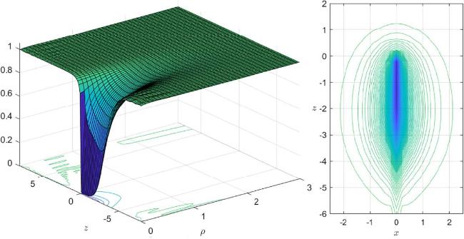
Figure 1. Higgs modulus and its contour of the Type I half-dyon for n = 1 and η = 0.1. |
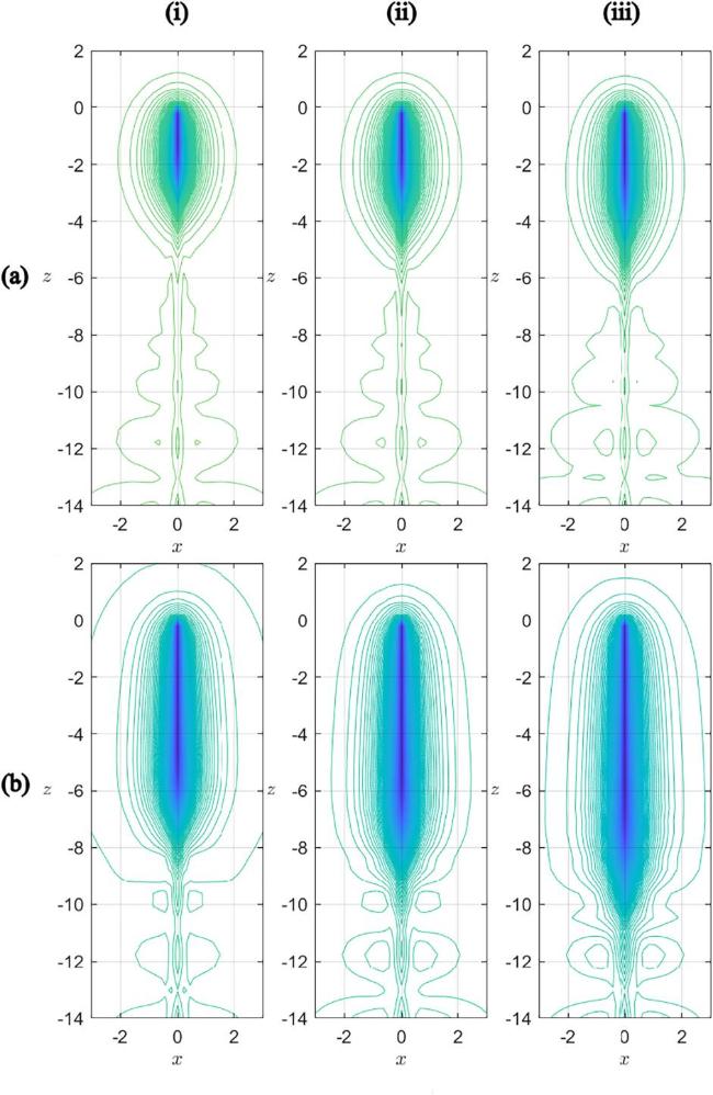
Figure 2. Higgs modulus contour of the Type I half-dyon for (a) n = 1 and (b) n = 2, at (i) η = 0, (ii) η = 0.3, and (iii) η = 0.4. |
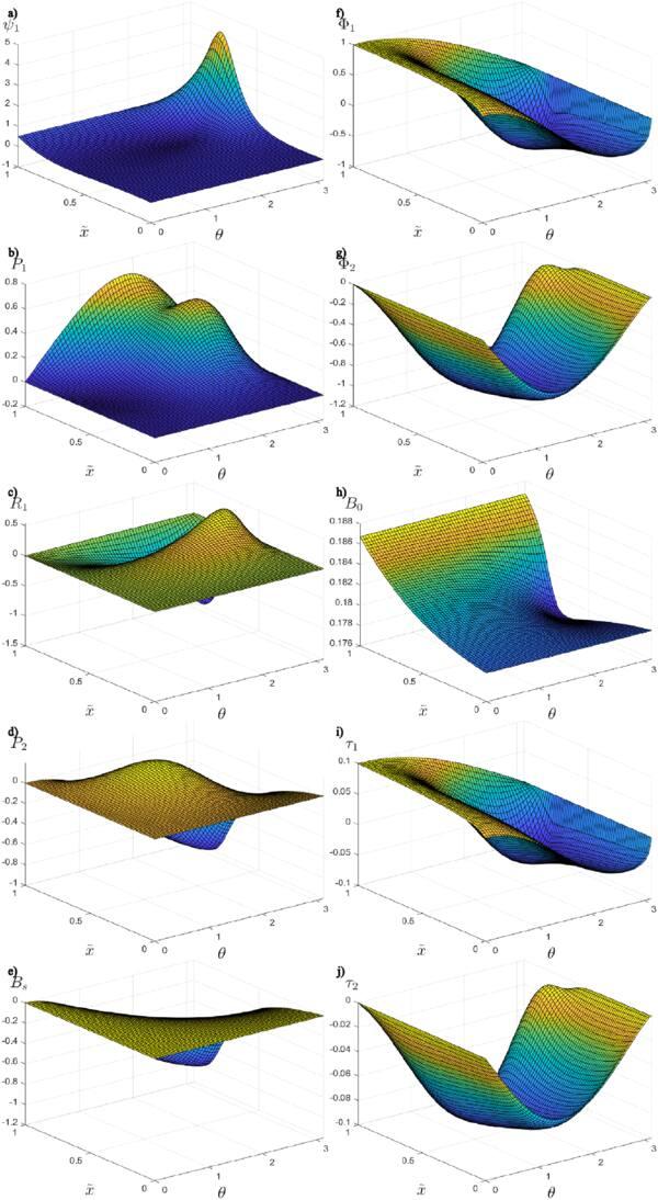
Figure 3. Profile functions (a) ψ1, (b) P1, (c) R1, (d) P2, (e) Bs, (f) Φ1, (g) Φ2, (h) ${\tilde{B}}_{0}$, (i) τ1 and (j) τ2, of Type I half-dyon for n = 1, η = 0.1, over the region of $0\,\leqslant \,\tilde{x}\,\leqslant \,1$, 0 ≤ θ ≤ π. |
The weighted energy density ϵW and its contour of the half-dyon solution when n = 1, η = 0.1 is plotted in figure 4. The weighted energy density shows an elongated balloon with the negative z-axis as its axis of symmetry, been blown from its opening at the origin. The results are in tandem with figure 1 and confirms that the half-dyon is concentrated along the negative z-axis, extending from the origin at r = 0 over a finite length.
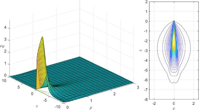
Figure 4. Weighted energy density and its contour of the Type I half-dyon for n = 1 and η = 0.1. |
From figure 5, it is obvious that besides magnetic charge density, the half-dyon carries electric charge density that is concentrated along the negative z-axis near the origin, together with ‘electric’ neutral charge density. The magnetic field lines and ‘magnetic’ neutral field lines of the half-dyon are shown in figure 6. While the magnetic field lines represent that of an object with finite magnetic charge qm along the negative z-axis extending from the origin, the plot of ‘magnetic’ neutral field lines suggests that there are finite zm concentration in the lower space. The upper part possesses positive zm whereas the lower part possesses negative zm adjacently, giving an overall net zero ‘magnetic’ neutral charge for the system.
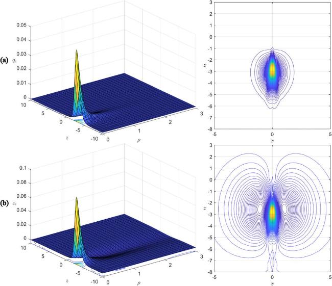
Figure 5. (a) Weighted electric charge density with its contour; and (b) weighted ‘electric’ neutral charge density with its contour, of the half-dyon solutions with n = 1, η = 0.1. |
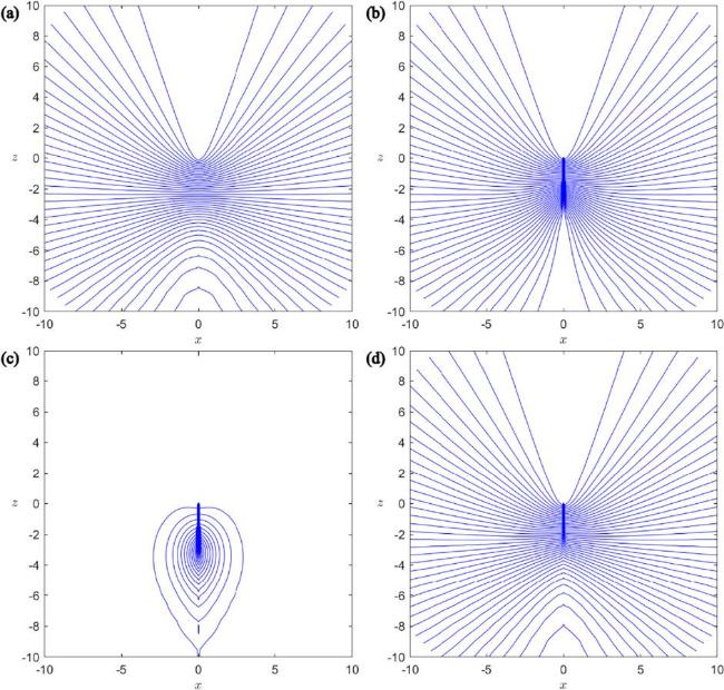
Figure 6. (a) U(1) magnetic field lines, (b) SU(2) magnetic field lines, (c) ‘magnetic’ neutral field lines and (d) ‘em’ magnetic field lines of the half-dyon solutions with n = 1, η = 0.1. |
To confirm the exact picture of the charges, we consider again equations (43 ), (49 ) and (51 ), with the radius of S2 now varies with dimensionless coordinate x. The functions of qm(x), qe(x), zm(x) and ze(x) in units of 4π/e versus x of half-dyon with n = 1 and various η are then plotted in figure 7. As expected, qm and qe rises from zero at x = 0 to 2π/e and maximal qe(max) respectively as x → ∞. For zm and ze, they both rises from zero at x = 0 to a maximal value at intermediate x before declining to zero as x → ∞. This shows that there exists equal amount of positive and negative charges at intermediate x but as x → ∞, zm → 0 and ze → 0. These phenomena are also observed for the case of n = 2, 3 and similar statement are presented in section 4 .
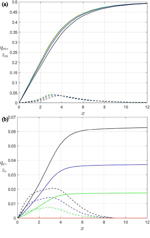
Figure 7. Functions of (a) magnetic charge ${q}_{m}\left(x\right)$ (solid) and ‘magnetic’ neutral charge ${z}_{m}\left(x\right)$ (dash-dotted), and (b) electric charge ${q}_{e}\left(x\right)$ (solid) and ‘electric’ neutral charge ${z}_{e}\left(x\right)$ (dash-dotted) versus x; for the Type I half-dyon solutions with n = 1, η = 0 (red), η = 0.2 (green), η = 0.3 (blue), and η = 0.4 (black). |
From the above statement, this means that the conditions of zm and ze approaching zero at large x do not indicate that the neutral charge densities are zero over all space, but they exist in intermediate region. Again from figure 7, the strength of these neutral charge densities in intermediate region are noticeably small, but not negligible. One may wonder if these are numerical errors but repeated calculations show that they are not. A possible remedy is to increase the accuracy of numerical solutions, i.e. consider a grid size of, say 120 × 110. This will be carried out in another work, but that will mean consumption of gigantic computational resources. In short the occurrence of neutral charge densities in the half-dyon solutions would demand further in-depth investigations.
Hence our solutions indicate that if a monopole undergoes distortion (due to excitation), neutral charge densities (with minute strength) would emerge, but the overall neutral charges would remain zero. There is however a crucial difference between zm and ze. For zm, its positive charge and negative charge are adjacently distributed along the negative z-axis, figure 6(c). For ze, the positive charges are distributed along the negative z-axis extending from the origin, while its negative charge are distributed along a finite tube encircling the positive charge, figure 5(b).
Next, the Type II solution is obtained by applying the boundary conditions (26 ), (29 ), (30 ), and (31 ). We similarly perform analytic calculation of total magnetic charge of Type II solutions using equations (43 )–(45 ) and obtain
$\begin{eqnarray}{q}_{m}=-\frac{2n\pi }{e},\,\,{q}_{m}^{\,\rm{upper}\,}=-\frac{2n\pi }{e},\,\,{q}_{m}^{\,\rm{lower}\,}=0.\end{eqnarray}$
This implies that the Type II half-dyon solution contains magnetic charge of −2nπ/e and distributes along the positive z-axis. Type II solution clearly differs from the Type I solution which has +2nπ/e and lies along the negative z-axis. figure 8 shows the Higgs modulus and its contour of Type II half-dyon solution at n = 1, η = 0.1. We also show the three-dimensional models of both the Type I and Type II half-dyons for comparison in figure 9. Both the magnetic and ‘magnetic’ neutral charges of Type II half-dyons are plotted in figure 10 which confirms our analysis that the magnetic charges are negative-valued.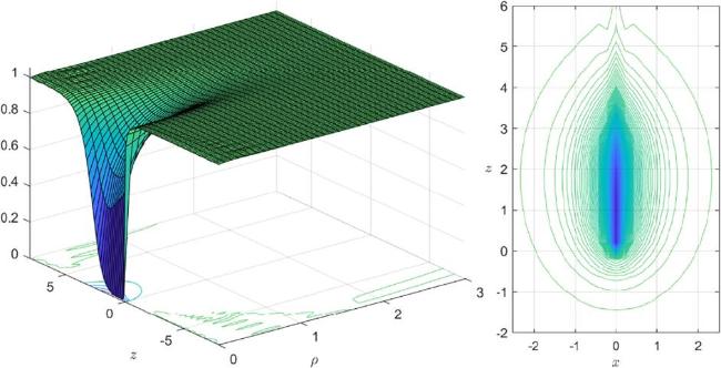
Figure 8. Higgs modulus and its contour of the Type II half-dyon for n = 1 and η = 0.1. |
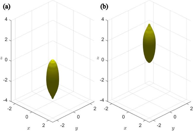
Figure 9. Three-dimensional models of the (a) Type I and (b) Type II half-dyons for n = 1 and η = 0.1. |
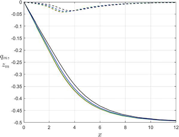
Figure 10. Functions of magnetic charge ${q}_{m}\left(x\right)$ (solid) and ‘magnetic’ neutral charge ${z}_{m}\left(x\right)$ (dash-dotted) for the Type II half-dyon solutions with n = 1, η = 0 (red), η = 0.2 (green), η = 0.3 (blue), and η = 0.4 (black). |
The Type II solutions have the exact same critical value ηc as their corresponding Type I solutions, which are 0.5001, 0.5005 and 0.1726 for n = 1, 2 and 3 respectively. Despite the opposite magnetic charge, both types of solutions share identical values for electric qe and ‘electric’ neutral ze charges. Comparison of figures 1 and 8 demonstrates that, in terms of structure, Type II half-dyons are perfect mirror images of Type I half-dyons across the $\rho =\sqrt{{x}^{2}+{y}^{2}}$ plane. These findings imply that the emergence of magnetic monopoles (or dyons) may occur in pairs, hinting at the potential for monopole pair production.
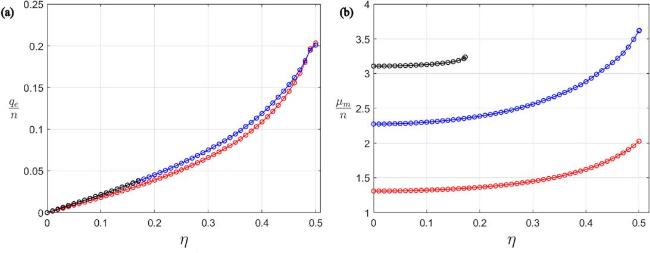
The plots of total electric charge per n, qe/n and magnetic dipole moment per n (μm/n) versus η are shown in figure 11. In general, the solutions possess a minimum value for qe/n and μm/n when η = 0, followed by an (approximately) quadratic increase until they reach their critical values at η = ηc. Hence overall the half-dyon solutions in WS theory possess almost similar pattern as the half-dyon in SU(2) YMH theory [21]. This is not surprising since the WS theory contains the SU(2) group. Selected values of qe and μm/n for the Type I half-dyon configurations are tabulated in table 1 for n = 1 to n = 3. For Type II half-dyon, it has exactly the same electric charge, ‘electric’ netural charge, and magnetic dipole moment as Type I half-dyon. Hence giving the same graphical behavior. table 1 also shows that qe(max) for n = 1, 2 and 3 are 0.2167, 0.4195 and 0.1141 respectively.
Figure 11. Plots of (a) qe/n (in unit of 4π/e) versus η, (b) μm/n (in unit of 1/e) versus η; of the Type I half-dyon solutions for n = 1 (red), n = 2 (blue) and n = 3 (black). |
Table 1. Selected values for electric charge qe in unit of 4π/e and magnetic dipole moment per n (μm/n) in unit of 1/e of the Type I half-dyon solution at physical Weinberg angle ${\sin }^{2}{\theta }_{\,\rm{W}\,}=0.2229$ and Higgs self-coupling constant β = 0.778 188 33 for φ-winding number 1 ≤ n ≤ 3. |
| n = 1 | |||||||||||
| | |||||||||||
| η | 0 | 0.05 | 0.10 | 0.15 | 0.20 | 0.25 | 0.30 | 0.35 | 0.40 | 0.45 | 0.5001 |
| qe | 0 | 0.0089 | 0.0181 | 0.0280 | 0.0388 | 0.0511 | 0.0658 | 0.0842 | 0.1088 | 0.1455 | 0.2167 |
| μm/n | 1.3101 | 1.3131 | 1.3225 | 1.3389 | 1.3637 | 1.3991 | 1.4488 | 1.5187 | 1.6196 | 1.7718 | 2.0291 |
| | |||||||||||
| n = 2 | |||||||||||
| | |||||||||||
| η | 0 | 0.05 | 0.10 | 0.15 | 0.20 | 0.25 | 0.30 | 0.35 | 0.40 | 0.45 | 0.5005 |
| qe | 0 | 0.0203 | 0.0412 | 0.0632 | 0.0871 | 0.1138 | 0.1449 | 0.1825 | 0.2306 | 0.2989 | 0.4195 |
| μm/n | 2.2744 | 2.2811 | 2.3014 | 2.3364 | 2.3878 | 2.4589 | 2.5594 | 2.6960 | 2.8816 | 3.1617 | 3.6229 |
| | |||||||||||
| n = 3 | |||||||||||
| | |||||||||||
| η | 0 | 0.05 | 0.10 | 0.15 | 0.1726 | ||||||
| qe | 0 | 0.0310 | 0.0627 | 0.0961 | 0.1141 | ||||||
| μm/n | 3.1107 | 3.1157 | 3.1329 | 3.1739 | 3.2407 | ||||||
Here we also elaborate on the Type I half-dyon solution with η = 0, n = 2, which is basically an electrically neutral monopole system that possesses magnetic charge 4π/e. The half-monopole is considered as an excited state of Cho–Maison monopole, hence sharing the same topological stability as Cho–Maison monopole. Because it is an excited state, it is expected to eventually lose energy to reach the lower energy state of a spherically symmetric Cho–Maison monopole. In comparison with the spherically symmetric Cho–Maison monopole [23] (which also possesses magnetic charge 4π/e), our solution with axial symmetry can be viewed as a superposition of two half-monopoles (hereon denoted as two-half-monopole). Besides symmetry, there exists some differences between the two-half-monopole and the Cho–Maison monopole. First the Cho–Maison monopole has absolutely no neutral charge (‘electric’ and ‘magnetic’). The two-half-monopole here possesses net zero neutral charge, as dictated by the boundary condition (25 ). However at finite r there are neutral charge densities which consists of equal amount of positive and negative neutral charge. In terms of physical structure, the two half-monopole has a distorted teardrop shape while Cho–Maison monopole possesses spherical symmetry. This indicates that the distortion of Cho–Maison monopole might lead to emergence of neutral charge density, though asymptotically the total neutral charge is zero.
6. Conclusions
Building from the ground work of generalized Type I and Type II half-dyon in SU(2) YMH theory [21], we study in this paper generalized Type I and Type II half-dyon in WS theory. By considering correct dimensions of the theory with physical Weinberg angle ${\sin }^{2}{\theta }_{\,\rm{W}\,}=0.2229$, Higgs self-coupling constant β = 0.778 188 33, φ-winding number 1 ≤ n ≤ 3 and electric charge parameter 0 ≤ η ≤ ηc, our analysis thoroughly explores fundamental properties such as magnetic charge, neutral charge, and magnetic dipole moment for the half-dyon solutions. These generalized half-dyon in WS theory are quite similar to the generalized half-dyon in SU(2) YMH theory, but with 1 ≤ n ≤ 4. Nevertheless, generalized half-dyon in WS theory does possess extra properties that are not present in their counterpart in SU(2) YMH theory.
The Type I half-dyon solution is a finite length object distributed along the negative z-axis extending from the origin. It possesses net magnetic charge 2nπ/e, electric charge 0 ≤ qe ≤ qe(max) and zero net neutral (electric and magnetic) charge. Structure wise, the Type II half-dyon is similar to Type I but distributed along the positive z-axis with a net magnetic charge of −2nπ/e. The electric charge qe and zero net neutral (electric and magnetic) charge of Type II half-dyon solutions are the same as their Type I counterparts under identical conditions. Although the generalized half-dyon solutions possess net zero neutral (electric and magnetic) charge, calculations reveal the presence of neutral (electric and magnetic) charge densities at intermediate regions, albeit with notably small strengths, prompting a need for further extensive investigations.
The generalized half-dyon solutions in this paper possess important distinctive properties as compared to the Cho–Maison MAP solutions in [45]. The Cho–Maison MAP are separate entities with finite separation, where the positive pole (+4π/e) is situated in the upper hemisphere and the negative pole (−4π/e) in the lower hemisphere. Although the Cho–Maison MAP systems are axially symmetrical, the poles themselves has spherical shape indicating they are fundamentally spherically symmetric Cho–Maison monopoles [23]. The novel Type I and Type II half-dyon system here are single entities situated near the origin with magnetic charge +2nπ/e (Type I) and −2nπ/e (Type II). The special case of n = 2 corresponding to an axially symmetric full Cho–Maison monopole, shows for the first time that a full Cho–Maison monopole can undergo distortion and possesses a tear-drop shape. The presence of both Type I and Type II half-dyon solutions supports the idea that Cho–Maison monopoles (or dyons) could appear in pairs, a concept further supported by the results of Cho–Maison MAP with finite separation in [45]. These two results signify the possibility of magnetic monopole pair production.