


1. Introductions
The gauge/gravity duality is believed to be a giant leap in understanding quantum gravity [1–3]. Several important developments were proposed afterward. From the gauge/gravity duality, a holographic interpretation of entanglement entropy in conformal field theory was provided and was soon generalized to black hole entanglement entropy [4–6]. The proposal of a chaos bound has linked black hole horizon physics with quantum chaos [7], i.e.
$\begin{eqnarray}{\lambda }_{L}\leqslant \frac{2\pi {k}_{{\rm{B}}}T}{\hslash },\end{eqnarray}$
where λL is the Lyapunov exponent, T is the temperature of the system, and in the case of a black hole, it corresponds to the Hawking temperature TH. This bound is saturated for theories with anti-de Sitter/conformal field theory duality. Therefore, when this chaos bound is saturated, it is speculated that the system will necessarily have an Einstein gravity dual, or at least be near its horizon [7, 8]. Another famous example of this bound being saturated is the Sachdev-Ye-Kitaev (SYK) model [9–13], and the low-energy properties of the SYK model are dual to Jackiw-Teitelboim gravity [14, 15].In the chaos bound proposal, the authors of [7] introduced a technical tool, the out-of-time-ordered commutator (OTOC), to obtain the Lyapunov exponent, which is characteristic of capturing the quantum chaos behavior. The OTOC is defined by [7]
$\begin{eqnarray}{\tilde{C}}_{T}(t)\equiv -\langle {[W(t),V(0)]}^{2}\rangle ,\end{eqnarray}$
where $\langle \cdot \rangle ={Z}^{-1}{\rm{tr}}[{{\rm{e}}}^{-\beta H}\cdot ]$ denotes the thermal expectation value at temperature T = β−1 and $Z={\rm{tr}}[{{\rm{e}}}^{-\beta H}]$ is the partition function. For fermionic operators, the commutator [W, V] is replaced by the anti-commutator {W, V} [16]. The OTOC can be used to diagnose the effects of serial perturbations V and W. If one chooses V = p and W = q(t), then ${\tilde{C}}_{T}$ becomes the Poisson bracket, and in the classical limit it scales as $\exp ({\lambda }_{L}t)$; it diagnoses the butterfly effect if λL > 0. Originally, the OTOC was introduced by Larkin and Ovchinnikov to reduce the field-current relation in a superconductor to a simpler artificial single-electron problem [17]. In [7], the authors propose to consider $\begin{eqnarray}{C}_{T}(t)=-\langle {[yW(t),yV]}^{2}\rangle ,\end{eqnarray}$
where ${y}^{4}=\frac{1}{Z}{{\rm{e}}}^{-\beta H}$. CT(t) grows as ${{\rm{e}}}^{{\lambda }_{L}t}$ at early times and generally saturates at long times (known as the Ehrenfest time).Ever since the chaos bound proposal, there have been many efforts and attempts to verify it via OTOC. For example, besides the SYK model and Jackiw-Teitelboim gravity, studies have been conducted on the BTZ black hole [18–20], the Kerr-AdS4 black hole [21], and the Myers-Perry-AdS5 black hole [22]. Their chaotic behaviors are diagnosed by OTOC, and holographic dual models are proposed when the chaos bound is saturated.
There is another case: a semiclassical particle moving near the horizon of a Schwarzschild black hole, where the chaos bound may also be saturated [23, 24]. This Lyapunov exponent arises from the classical motion inside an effective inverse harmonic potential near the black hole horizon, and the surface gravity of the black hole, which equals 2πkBTH/ℏ, provides a universal Lyapunov exponent and identical to the upper chaos bound [23]. One may then ask an interesting question: can this hold for quantum particles beyond the semiclassical approximation?
In this article, we shall consider the cases of quantum scalar and spinor fields moving in the background of a Schwarzschild black hole and examine the chaos bound by directly calculating their OTOCs. Here we choose V(0) ≡ p(0) and W(t) ≡ x(t) = eiHtx(0)e−iHt. In the energy representation, the OTOC can be written as [25]
$\begin{eqnarray}{C}_{T}(t)=\displaystyle \sum _{n}{f}_{n}{c}_{n}(t),\end{eqnarray}$
where ${f}_{n}=\frac{1}{{{\rm{e}}}^{{E}_{n}}+1}$ for Fermion and ${f}_{n}=\frac{1}{{{\rm{e}}}^{{E}_{n}}-1}$ for Boson. $\begin{eqnarray}{c}_{n}(t)=\displaystyle \sum _{m}{b}_{nm}(t){b}_{nm}^{* }(t),\end{eqnarray}$
$\begin{eqnarray}\begin{array}{rcl}{b}_{nm}(t) & = & -{\rm{i}}\langle n| [yx(t),yp]| m\rangle \\ & = & -{\rm{i}}\displaystyle \sum _{k}({{\rm{e}}}^{{\rm{i}}{E}_{nk}t-\beta {E}_{nk}/4}{x}_{nk}{{\rm{e}}}^{-\beta {E}_{km}/4}{p}_{km}\\ & & -{{\rm{e}}}^{{\rm{i}}{E}_{km}t-\beta {E}_{km/4}}{p}_{nk}{{\rm{e}}}^{-\beta {E}_{nk}/4}{x}_{km}),\end{array}\end{eqnarray}$
where Enm = En − Em and En is the energy level. xnm ≡ ⟨n∣x∣m⟩, and pnm ≡ ⟨n∣p∣m⟩.By numerically calculating the OTOCs along the radial direction for both the massive scalar field and the spinor field, we find that the Lyapunov exponents for both fields obtained from the OTOCs are below the chaos bound and mainly arise from the bound states near the horizon. Furthermore, the Lyapunov exponent of the spinor field is larger than that of the scalar field.
Besides theoretical simulations for black hole geometry, several promising condensed matter systems for mimicking black hole physics have been proposed. For example, the black hole or curved space analogs have been proposed in transsonic fluid flow [26], Bose–Einstein condensation [27, 28], magnonic systems [29], fractional quantum Hall effects [30–34], graphene [35, 36], deformed crystals [37], Weyl semimetals [38–43], and strange metals [44–46]. Additionally, with progress in measuring OTOCs in cold atom systems [47–49], we believe our results may shed light on the study of quantum chaos behavior in black hole physics and holography.
This paper is organized as follows: In section 2 , we set up the radial equations for massive scalar and spinor fields in Schwarzschild spacetime. The radial equations reduce to effective one-dimensional Schrödinger equations with barrier potentials. In section 3 , we numerically solve the wave functions for the radial equations and calculate the OTOCs for scalar and spinor fields. The temperature dependence, energy cutoff dependence, and rest mass dependence of the Lyapunov exponents in the numerical calculations are also discussed. The last part is devoted to conclusions.
2. Radial equations for massive scalar and spinor fields in the Schwarzschild spacetime
2.1. Massive scalar fields
The standard metric of the Schwarzschild spacetime in Schwarzschild coordinates reads 11 ) becomes an effective one-dimensional Schrödinger equation,
$\begin{eqnarray}{\rm{d}}{s}^{2}=\left(1-\frac{{r}_{0}}{r}\right){\rm{d}}{t}^{2}-\frac{{\rm{d}}{r}^{2}}{1-\frac{{r}_{0}}{r}}-{r}^{2}\left({\rm{d}}{\theta }^{2}+{\sin }^{2}\theta {\rm{d}}{\varphi }^{2}\right),\end{eqnarray}$
where r0 = 2M is the Schwarzschild radius and M is the black hole mass. And the action for a real massive scalar field φ is $\begin{eqnarray}{S}_{\mathrm{sc}}=\int \sqrt{-g}\left(\displaystyle \frac{1}{2}{g}^{\mu \nu }{\partial }_{\mu }\phi {\partial }_{\nu }\phi -\displaystyle \frac{{m}_{SC}^{2}}{2}{\phi }^{2}\right){{\rm{d}}}^{4}x.\end{eqnarray}$
The corresponding equation of motion reads $\begin{eqnarray}\sqrt{-g}{g}^{00}\ddot{\phi }+{\partial }_{i}\left(\sqrt{-g}{g}^{{\rm{i}}j}{\partial }_{j}\phi \right)+{m}_{sc}^{2}\sqrt{-g}\phi =0,\end{eqnarray}$
where $\dot{\phi }={\partial }_{0}\phi $ and msc is the mass of the scalar field. The static solution of φ has the form $\begin{eqnarray}{{\rm{e}}}^{\pm {\rm{i}}Et}{Y}_{{lm}}(\theta ,\varphi ){f}_{l}(E,r),\end{eqnarray}$
where Ylm are the spherical harmonics. And the radial equation becomes $\begin{eqnarray}\begin{array}{l}{E}^{2}\frac{r}{r-{r}_{0}}{f}_{l}(E,r)-{M}^{2}{f}_{l}(E,r)\\ +\frac{1}{{r}^{2}}\frac{{\rm{d}}}{{\rm{d}}r}\left(r(r-{r}_{0})\frac{{\rm{d}}{f}_{l}(E,r)}{{\rm{d}}r}\right)-\frac{l(l+1)}{{r}^{2}}{f}_{l}(E,r)=0.\end{array}\end{eqnarray}$
By redefining several dimensionless variables, $\begin{eqnarray}\begin{array}{rcl}\mu & = & {m}_{\mathrm{sc}}{r}_{0},\quad \epsilon =E{r}_{0},\\ z & = & \displaystyle \frac{r}{{r}_{0}}+{\mathrm{ln}}\,\left(\displaystyle \frac{r}{{r}_{0}}-1\right),\quad {\psi }_{l}(\epsilon ,z)=r{f}_{l}(E,r),\end{array}\end{eqnarray}$
the radial equation ( $\begin{eqnarray}-\frac{{{\rm{d}}}^{2}{\psi }_{l}(\epsilon ,z)}{{\rm{d}}{z}^{2}}+{V}_{l}(z){\psi }_{l}(\epsilon ,z)={\epsilon }^{2}{\psi }_{l}(\epsilon ,z),\end{eqnarray}$
where the potential has the form [51] $\begin{eqnarray}{V}_{l}(z)=\frac{r(z)-{r}_{0}}{r(z)}\left({\mu }^{2}+\frac{l(l+1){r}_{0}^{2}}{{r}^{2}(z)}+\frac{{r}_{0}^{3}}{{r}^{3}(z)}\right).\end{eqnarray}$
We plot several examples of Vl(z) in figure 1. From these examples one can notice that Vl(z) → 0 for z → −∞ and Vl(z) → μ2 for z → +∞ which leads to the following asymptotic behavior of the radial equation,
$\begin{eqnarray}-\frac{{{\rm{d}}}^{2}{\psi }_{l}(\epsilon ,z)}{{\rm{d}}{z}^{2}}+{\mu }^{2}{\psi }_{l}(\epsilon ,z)={\epsilon }^{2}{\psi }_{l}(\epsilon ,z),\,\,\,\,z\to +\infty .\end{eqnarray}$
$\begin{eqnarray}-\frac{{{\rm{d}}}^{2}{\psi }_{l}(\epsilon ,z)}{{\rm{d}}{z}^{2}}={\epsilon }^{2}{\psi }_{l}(\epsilon ,z),\,\,\,\,z\to -\infty .\end{eqnarray}$
For $\left|\epsilon \right|\gt \left|\mu \right|$, it induces the boundary condition $\begin{eqnarray}\begin{array}{rcl}{\psi }_{l}^{(1)}(\epsilon ,z) & = & \cos (\sqrt{{\epsilon }^{2}-{\mu }^{2}}z),\,\,\,\,z\to +\infty .\\ {\psi }_{l}^{(1)}(\epsilon ,z) & = & \cos (\epsilon z),\,\,\,\,z\to -\infty .\end{array}\end{eqnarray}$
$\begin{eqnarray}\begin{array}{rcl}{\psi }_{l}^{(2)}(\epsilon ,z) & = & \sin (\sqrt{{\epsilon }^{2}-{\mu }^{2}}z),\,\,\,\,z\to +\infty .\\ {\psi }_{l}^{(2)}(\epsilon ,z) & = & \sin (\epsilon z),\,\,\,\,z\to -\infty .\end{array}\end{eqnarray}$
There is a pair of orthogonal solutions ${\psi }_{l}^{(1)}$ and ${\psi }_{l}^{(2)}$ for $\left|\epsilon \right|\gt \left|\mu \right|$, which correspond to ${f}_{l}^{(1)}$ and ${f}_{l}^{(2)}$. For the bound states near the horizon, $\left|\epsilon \right|\lt \left|\mu \right|$, it induces the boundary condition
$\begin{eqnarray}\begin{array}{rcl}{\psi }_{l}(\epsilon ,z) & = & 0,\quad z\to +\infty .\\ {\psi }_{l}(\epsilon ,z) & = & \cos (\epsilon z),\quad z\to -\infty .\end{array}\end{eqnarray}$

Figure 1. Examples of Vl(z) for μ = 1. (a) l = 0, and (b) l = 3. |
2.2. Massive spinor fields
The action of a massive spinor field reads 7 ) can be rewritten as 22 ) has the form
$\begin{eqnarray}\begin{array}{l}{S}_{\mathrm{sp}}=\int \sqrt{-g}\\ \left[\displaystyle \frac{{\rm{i}}}{2}\left(\bar{\psi }{\gamma }^{(\nu )}{{\rm{e}}}_{(\nu )}^{\mu }{\nabla }_{\mu }\,\psi -{\nabla }_{\mu }\,\bar{\psi }{{\rm{e}}}_{(\nu )}^{\mu }{\gamma }^{(\nu )}\psi \right)-{m}_{\mathrm{sp}}\bar{\psi }\psi \right]{{\rm{d}}}^{4}x,\end{array}\end{eqnarray}$
where msp is the mass of the spinor field, ${{\rm{e}}}_{(\nu )}^{\mu }$ are the vielbein fields, and ∇μ are the covariant derivatives defined by $\begin{eqnarray}\begin{array}{rcl}{{\rm{\nabla }}}_{\mu }\,\psi & = & \left({\partial }_{\mu }\psi +{\omega }_{\mu }\psi \right),\quad {{\rm{\nabla }}}_{\mu }\,\bar{\psi }=\left({\partial }_{\mu }\bar{\psi }-\bar{\psi }{\omega }_{\mu }\right),\\ {\omega }_{\mu } & = & \frac{1}{8}{\omega }_{(\nu )(\rho )\mu }\left[{\gamma }^{(\nu )},{\gamma }^{(\rho )}\right],\\ {\omega }_{(\nu )(\rho )\mu } & = & {g}_{\sigma \tau }{{\rm{e}}}_{(\nu )}^{\tau }\left({\partial }_{\mu }{{\rm{e}}}_{(\rho )}^{\sigma }+{{\rm{\Gamma }}}_{\mu \lambda }^{\sigma }{{\rm{e}}}_{(\rho )}^{\lambda }\right),\end{array}\end{eqnarray}$
where ω(ν)(ρ)μ are the spin connections and ${{\rm{\Gamma }}}_{\mu \lambda }^{\sigma }$ are the Christoffel symbols. ${{\rm{e}}}_{(\rho )}^{\mu }{{\rm{e}}}_{(\sigma )}^{\nu }\left\{{\gamma }^{(\rho )},{\gamma }^{(\sigma )}\right\}=2{g}^{\mu \nu }$. The Dirac equation in the curved spacetime reads $\begin{eqnarray}{\rm{i}}{\gamma }^{(\nu )}{{\rm{e}}}_{(\nu )}^{\mu }\left({\partial }_{\mu }+{\omega }_{\mu }\right)\psi -{m}_{\mathrm{sp}}\psi =0.\end{eqnarray}$
By introducing [52] $\begin{eqnarray}\begin{array}{rcl}r & = & R+\frac{{M}^{2}}{4R}+M=R+\frac{{r}_{0}^{2}}{16R}+\frac{{r}_{0}}{2},\\ R & = & \sqrt{{x}^{2}+{y}^{2}+{z}^{2}},\end{array}\end{eqnarray}$
the Schwarzschild metric equation ( $\begin{eqnarray}{g}_{00}=\frac{{\left(1-\frac{{r}_{0}}{4R}\right)}^{2}}{{\left(1+\frac{{r}_{0}}{4R}\right)}^{2}},\quad {g}_{ii}=-{\left(1+\frac{{r}_{0}}{4R}\right)}^{4},\end{eqnarray}$
$\begin{eqnarray}{g}_{\mu \nu }=0,\quad \mu \ne \nu ,\end{eqnarray}$
where the Latin coordinate index i corresponds to the spatial coordinates. Then the vielbein fields are $\begin{eqnarray}{{\rm{e}}}_{(0)}^{0}=\frac{1+\frac{{r}_{0}}{4R}}{1-\frac{{r}_{0}}{4R}},\quad {{\rm{e}}}_{(k)}^{k}={\left(1+\frac{{r}_{0}}{4R}\right)}^{-2},\end{eqnarray}$
$\begin{eqnarray}{{\rm{e}}}_{(\nu )}^{\mu }=0,\quad \mu \ne \nu .\end{eqnarray}$
The Christoffel symbols are: $\begin{eqnarray}{{\rm{\Gamma }}}_{\mu \nu }^{0}=\frac{{r}_{0}}{2{R}^{3}}\frac{1}{\left(1-\frac{{r}_{0}}{4R}\right)\left(1+\frac{{r}_{0}}{4R}\right)}\left(\begin{array}{cccc}0 & x & y & z\\ x & 0 & 0 & 0\\ y & 0 & 0 & 0\\ z & 0 & 0 & 0\end{array}\right),\end{eqnarray}$
$\begin{eqnarray}{{\rm{\Gamma }}}_{\mu \nu }^{1}=\frac{{r}_{0}}{2{R}^{3}}\frac{1}{1+\frac{{r}_{0}}{4R}}\left(\begin{array}{cccc}\frac{1-\frac{{r}_{0}}{4R}}{{\left(1+\frac{{r}_{0}}{4R}\right)}^{6}}x & 0 & 0 & 0\\ 0 & -x & -y & -z\\ 0 & -y & x & 0\\ 0 & -z & 0 & x\end{array}\right),\end{eqnarray}$
$\begin{eqnarray}{{\rm{\Gamma }}}_{\mu \nu }^{2}=\frac{{r}_{0}}{2{R}^{3}}\frac{1}{1+\frac{{r}_{0}}{4R}}\left(\begin{array}{cccc}\frac{1-\frac{{r}_{0}}{4R}}{{\left(1+\frac{{r}_{0}}{4R}\right)}^{6}}y & 0 & 0 & 0\\ 0 & y & -x & 0\\ 0 & -x & -y & -z\\ 0 & 0 & -z & y\end{array}\right),\end{eqnarray}$
$\begin{eqnarray}{{\rm{\Gamma }}}_{\mu \nu }^{3}=\frac{{r}_{0}}{2{R}^{3}}\frac{1}{1+\frac{{r}_{0}}{4R}}\left(\begin{array}{cccc}\frac{1-\frac{{r}_{0}}{4R}}{{\left(1+\frac{{r}_{0}}{4R}\right)}^{6}}z & 0 & 0 & 0\\ 0 & z & 0 & -x\\ 0 & 0 & z & -y\\ 0 & -x & -y & -z\end{array}\right).\end{eqnarray}$
And the spin connections read $\begin{eqnarray}{\omega }_{0}=\frac{{r}_{0}}{8{R}^{3}}{\left(1+\frac{{r}_{0}}{4R}\right)}^{-4}\left[{\gamma }^{(0)},\overrightarrow{x}\overrightarrow{\gamma }\right],\end{eqnarray}$
$\begin{eqnarray}{\omega }_{k}=\frac{{r}_{0}}{8{R}^{3}}{\left(1+\frac{{r}_{0}}{4R}\right)}^{-1}\left[{\gamma }^{(k)},\overrightarrow{x}\overrightarrow{\gamma }\right],\end{eqnarray}$
where $\overrightarrow{\gamma }\equiv \left({\gamma }^{(1)},{\gamma }^{(2)},{\gamma }^{(3)}\right)$ and $\overrightarrow{x}\overrightarrow{\gamma }\equiv {x}^{1}{\gamma }^{(1)}+{x}^{2}{\gamma }^{(2)}\,+{x}^{3}{\gamma }^{(3)}=x{\gamma }^{(1)}+y{\gamma }^{(2)}+z{\gamma }^{(3)}$. By choosing the Dirac representation for γ-matrices, the static solution for the Dirac equation ( $\begin{eqnarray}{\psi }_{Ejl{m}_{{\rm{t}}}}\left(t,R,\theta ,\varphi \right)=\left(\begin{array}{c}{F}_{jl}\left(E,R\right){{\rm{\Omega }}}_{jl{m}_{{\rm{t}}}}\left(\theta ,\varphi \right)\\ {\rm{i}}{G}_{{l}^{{\prime} }}\left(E,R\right){{\rm{\Omega }}}_{jl^{\prime} {m}_{{\rm{t}}}}\left(\theta ,\varphi \right)\end{array}\right){{\rm{e}}}^{-{\rm{i}}Et},\end{eqnarray}$
where E is the energy, j is the total angular momentum, mt is its projection; $l=j\pm \frac{1}{2}$ and $l^{\prime} =j\mp \frac{1}{2}$ are the orbital angular momenta, $\begin{eqnarray}{F}_{jl}=\frac{{f}_{jl}}{r{\left(1-\frac{{r}_{0}}{r}\right)}^{\frac{1}{4}}},\quad {G}_{i{l}^{{\prime} }}=\frac{{g}_{jl^{\prime} }}{r{\left(1-\frac{{r}_{0}}{r}\right)}^{\frac{1}{4}}}.\end{eqnarray}$
$\begin{eqnarray}{{\rm{\Omega }}}_{jl{m}_{{\rm{t}}}}\left(\theta ,\varphi \right)=\left(\begin{array}{c}{C}_{l,{m}_{{\rm{t}}}-\frac{1}{2},\frac{1}{2},\frac{1}{2}}^{j{m}_{{\rm{t}}}}{Y}_{l}^{{m}_{{\rm{t}}}-\frac{1}{2}}\left(\theta ,\varphi \right)\\ {C}_{l,{m}_{{\rm{t}}}+\frac{1}{2},\frac{1}{2},-\frac{1}{2}}^{j{m}_{{\rm{t}}}}{Y}_{l}^{{m}_{{\rm{t}}}+\frac{1}{2}}\left(\theta ,\varphi \right)\end{array}\right),\end{eqnarray}$
are the spherical spinors with ${C}_{l,{m}_{{\rm{t}}}\pm \frac{1}{2},\frac{1}{2},\mp \frac{1}{2}}^{j{m}_{{\rm{t}}}}$ been the Clebsch–Gordan coefficients. Then the radial Dirac equation reads $\begin{eqnarray}{H}_{r}(\kappa )\left(\begin{array}{c}{f}_{jl}\\ {g}_{jl^{\prime} }\end{array}\right)=E\left(\begin{array}{c}{f}_{jl}\\ {g}_{jl^{\prime} }\end{array}\right),\end{eqnarray}$
with $\begin{eqnarray}\kappa =l(l+1)-j(j+1)-\frac{1}{4},\end{eqnarray}$
$\begin{eqnarray}\begin{array}{rcl}{H}_{r}(\kappa ) & = & -{\rm{i}}{\sigma }^{(2)}\left(1-\frac{{r}_{0}}{r}\right)\frac{{\rm{d}}}{{\rm{d}}r},\\ & & +{\sigma }^{(1)}\frac{\kappa \sqrt{1-\frac{{r}_{0}}{r}}}{r}+{\sigma }^{(3)}\sqrt{1-\frac{{r}_{0}}{r}}m,\end{array}\end{eqnarray}$
where σ(i) are the Pauli matrices. By omitting the angular momentum indices j, l, ${l}^{{\prime} }$, and introducing the tortoise coordinate $\rho \left(z\right)+{\mathrm{ln}}\,\left(\rho \left(z\right)-1\right)=z$, the dimensionless variables $\rho =\frac{r}{{r}_{0}}$, ϵ = r0E, μ = r0msp, and making the transformation, $\begin{eqnarray}f=\sqrt{1+\frac{\mu }{\varepsilon }\sqrt{1-\frac{1}{\rho \left(z\right)}}}u,\end{eqnarray}$
then the radial equation for f reduces to [52] $\begin{eqnarray}-\frac{{{\rm{d}}}^{2}u}{{\rm{d}}{z}^{2}}+{V}_{\kappa }^{(u)}\left(\varepsilon ,z\right)u={\varepsilon }^{2}u,\end{eqnarray}$
with $\begin{eqnarray}\begin{array}{l}{V}_{\kappa }^{\left(u\right)}\left(\varepsilon ,z\right)=\frac{\mu {\left(\rho \left(z\right)-1\right)}^{\frac{3}{2}}-\kappa \varepsilon \rho \left(z\right)\sqrt{\rho \left(z\right)-1}}{2{\rho }^{\frac{9}{2}}\left(z\right)\left(\varepsilon +\mu \sqrt{\frac{\rho \left(z\right)-1}{\rho \left(z\right)}}\right)}\\ \quad +\frac{{\mu }^{2}\left(\rho \left(z\right)-1\right)-2\mu \varepsilon \sqrt{\left(\rho \left(z\right)-1\right)\rho \left(z\right)}}{16{\rho }^{5}\left(z\right){\left(\varepsilon +\mu \sqrt{\frac{\rho \left(z\right)-1}{\rho \left(z\right)}}\right)}^{2}}\\ \quad +{\mu }^{2}\frac{\rho \left(z\right)-1}{\rho \left(z\right)}+\kappa \frac{{\left(\rho \left(z\right)-1\right)}^{\frac{3}{2}}}{{\rho }^{\frac{7}{2}}\left(z\right)}+{\kappa }^{2}\frac{\rho \left(z\right)-1}{{\rho }^{3}\left(z\right)}.\end{array}\end{eqnarray}$
f and g are related by the transformation $\begin{eqnarray}f\to g,\quad \varepsilon \to -\varepsilon ,\quad \kappa \to -\kappa .\end{eqnarray}$
Therefore by transforming $\begin{eqnarray}g=\sqrt{1+\frac{\mu }{\varepsilon }\sqrt{1-\frac{1}{\rho \left(z\right)}}}v,\end{eqnarray}$
the radial equation for g reduces to $\begin{eqnarray}-\frac{{{\rm{d}}}^{2}v}{{\rm{d}}{z}^{2}}+{V}_{\kappa }^{(v)}\left(\varepsilon ,z\right)v={\varepsilon }^{2}v,\end{eqnarray}$
with $\begin{eqnarray}{V}_{\kappa }^{(v)}\left(\varepsilon ,z\right)={V}_{-\kappa }^{(u)}\left(-\varepsilon ,z\right).\end{eqnarray}$
We plot several examples of ${V}_{\kappa }^{(u)}\left(\varepsilon ,z\right)$ in figure 2.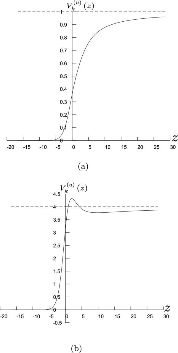
Figure 2. Examples of ${V}_{\kappa }^{(u)}\left(\varepsilon ,z\right)$ for (a) ε = 0.2, κ = −1, and μ = 1; (b) ε = 4, κ = 4, and μ = 2. |
Similar to the massive scalar field case, for ε > 0, ${V}_{\kappa }\left(\varepsilon ,z\right)\to 0$ for z → −∞ and ${V}_{\kappa }\left(\varepsilon ,z\right)\to {\mu }^{2}$ for z → +∞. And the corresponding boundary conditions are
$\begin{eqnarray}-\frac{{{\rm{d}}}^{2}u(\epsilon ,z)}{{\rm{d}}{z}^{2}}+{\mu }^{2}u(\epsilon ,z)={\epsilon }^{2}u(\epsilon ,z),\quad z\to +\infty .\end{eqnarray}$
$\begin{eqnarray}-\frac{{{\rm{d}}}^{2}u(\epsilon ,z)}{{\rm{d}}{z}^{2}}={\epsilon }^{2}u(\epsilon ,z),\quad z\to -\infty .\end{eqnarray}$
Considering the condition $\left|\epsilon \right|\gt \left|\mu \right|$, $\begin{eqnarray}\begin{array}{rcl}{u}^{(1)}(\epsilon ,z) & = & \cos (\sqrt{{\epsilon }^{2}-{\mu }^{2}}z),\quad z\to +\infty .\\ {u}^{(1)}(\epsilon ,z) & = & \cos (\epsilon z),\quad z\to -\infty .\end{array}\end{eqnarray}$
$\begin{eqnarray}\begin{array}{rcl}{u}^{(2)}(\epsilon ,z) & = & \sin (\sqrt{{\epsilon }^{2}-{\mu }^{2}}z),\quad z\to +\infty .\\ {u}^{(2)}(\epsilon ,z) & = & \sin (\epsilon z),\quad z\to -\infty .\end{array}\end{eqnarray}$
There is a pair of orthogonal solutions u(1) and u(2) for $\left|\epsilon \right|\gt \left|\mu \right|$ corresponding to ${F}_{jl}^{(1)}$ and ${F}_{jl}^{(2)}$. For the bound states near the horizon, $\left|\epsilon \right|\lt \left|\mu \right|$, it induces the boundary condition $\begin{eqnarray}\begin{array}{rcl}u(\epsilon ,z) & = & 0,\quad z\to +\infty .\\ u(\epsilon ,z) & = & \cos (\epsilon z),\quad z\to -\infty .\end{array}\end{eqnarray}$
It is the same for v(ε, z) when $\left|\epsilon \right|\gt \left|\mu \right|$; similarly, v(1) and v(2) corresponding to ${G}_{jl}^{(1)}$ and ${G}_{jl}^{(2)}$.3. OTOC and Lyapunov exponents of scalar and spinor fields in the Schwarzschild spacetime
The expectation value of an operator $\hat{O}$ of the radial direction for the scalar field is defined by [50]12 ). And for the spinor field it is defined by [52]35 ). Additionally, we have a pair of orthogonal solutions for the condition of $\left|\epsilon \right|\gt \left|\mu \right|$. For the scalar field 6 ), we consider the radial position $\hat{x}=r$ and the radial momentum $\hat{p}={\rm{i}}\partial /\partial r$. For the scalar field, the matrix elements are
$\begin{eqnarray}\langle m| \hat{O}| n\rangle =\displaystyle \sum _{l}{\int }_{{r}_{0}}^{\infty }\frac{{r}^{3}}{r-{r}_{0}}{f}_{l}^{* }({E}_{m},r)\hat{O}{f}_{l}({E}_{n},r){\rm{d}}r,\end{eqnarray}$
where fl(E, r) and r can be obtained according from equation ( $\begin{eqnarray}\begin{array}{l}\langle m| \hat{O}| n\rangle =\displaystyle \sum _{j}{\displaystyle \int }_{{r}_{0}}^{\infty }\frac{{r}^{2}{\rm{e}}r}{\sqrt{1-\frac{{r}_{0}}{r}}}\\ \left({F}_{jl}^{* }\left({E}_{m},r\right)\hat{O}{F}_{jl}\left({E}_{n},r\right)+{G}_{jl^{\prime} }^{* }\left(E,r\right)\hat{O}{G}_{jl^{\prime} }\left(E^{\prime} ,r\right)\right),\end{array}\end{eqnarray}$
and Fjl and Gjl are obtained from equation ( $\begin{eqnarray}{f}_{l}=\frac{1}{\sqrt{2}}({f}_{l}^{(1)}+{f}_{l}^{(2)}).\end{eqnarray}$
For the spinor field $\begin{eqnarray}\begin{array}{rcl}{F}_{jl} & = & \frac{1}{\sqrt{2}}({F}_{jl}^{(1)}+{F}_{jl}^{(2)}),\\ {G}_{jl} & = & \frac{1}{\sqrt{2}}({G}_{jl}^{(1)}+{G}_{jl}^{(2)}).\end{array}\end{eqnarray}$
Therefore, in the calculation of OTOC equation ( $\begin{eqnarray}{x}_{mn}=\displaystyle \sum _{l}{\int }_{{r}_{0}}^{\infty }\frac{{r}^{4}{\rm{d}}r}{r-{r}_{0}}{f}_{l}^{* }({E}_{m},r){f}_{l}({E}_{n},r),\end{eqnarray}$
$\begin{eqnarray}{p}_{mn}=\displaystyle \sum _{l}-{\rm{i}}{\int }_{{r}_{0}}^{\infty }\frac{{r}^{3}{\rm{d}}r}{r-{r}_{0}}{f}_{l}^{* }({E}_{m},r)\frac{\partial }{\partial r}{f}_{l}({E}_{n},r).\end{eqnarray}$
And for the spinor fields they are $\begin{eqnarray}\begin{array}{rcl}{x}_{mn} & = & \displaystyle \sum _{j}{\displaystyle \int }_{{r}_{0}}^{\infty }\frac{{r}^{3}{\rm{d}}r}{\sqrt{1-\frac{{r}_{0}}{r}}}({F}_{jl}^{* }\left({E}_{m},r\right){F}_{jl}\left({E}_{n},r\right)\\ & & +{G}_{jl^{\prime} }^{* }\left({E}_{m},r\right){G}_{jl^{\prime} }\left({E}_{n},r\right)),\end{array}\end{eqnarray}$
$\begin{eqnarray}\begin{array}{rcl}{p}_{mn} & = & \displaystyle \sum _{j}-{\rm{i}}{\displaystyle \int }_{{r}_{0}}^{\infty }\frac{{r}^{2}{\rm{d}}r}{\sqrt{1-\frac{{r}_{0}}{r}}}({F}_{jl}^{* }\left({E}_{m},r\right)\frac{\partial }{\partial r}{F}_{jl}\left({E}_{n},r\right)\\ & & +{G}_{jl^{\prime} }^{* }\left({E}_{m},r\right)\frac{\partial }{\partial r}{G}_{jl^{\prime} }\left({E}_{n},r\right)).\end{array}\end{eqnarray}$
We numerically solve the normalized wave functions for the radial equations (13 ) and (41 ) with the boundary conditions equation (18 ) for the scalar field and equation (50 ) for the spinor field. The solution of equation (45 ) can be obtained via the transformation equation (43 ).
We plot the typical OTOC diagrams for the scalar and spinor fields respectively in figure 3. The OTOCs for both fields grow exponentially at early times and saturate at large times (the Ehrenfest time) as expected. In the calculations, we have chosen μ = 5 and β = 10, and set ℏ = kB = 1. The Lyapunov exponent is conveniently obtained by taking the logarithm of CT(t); i.e. ${\mathrm{ln}}\,{C}_{T}(t)$ is linear with the slope being the Lyapunov exponent at early times. We find that when β = 10, the Lyapunov exponents for both the scalar and spinor fields are smaller than the chaos bound, which is 2π/β. The Lyapunov exponent of the spinor field is larger than that of the scalar field. Furthermore, the main contribution to the Lyapunov exponent arises from the bound states near the horizon, which is consistent with the semiclassical result that only considers the particle moving near the horizon [23, 24].
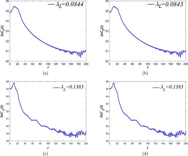
Figure 3. The diagrams of the OTOCs: μ = 5 and β = 10. The energy cutoff is chosen as ${E}_{{\rm{\min }}}=0.5$ and ${E}_{{\rm{\max }}}=100$. The red line regime is nearly linear, and its slope corresponds to the Lyapunov exponent. (a) and (b) are for the scalar fields while (c) and (d) are for the spinor fields. (a) and (c) are the total OTOCs while (b) and (d) only include the contributions of the bound states near the horizon. Therefore, the main part of the Lyapunov exponent arises from the bound states. |
In the numerical calculation, the energy ε is bounded by ${E}_{{\rm{\min }}}\lt \epsilon \lt {E}_{{\rm{\max }}}$, where ${E}_{{\rm{\min }}}$ is the minimum energy cutoff and ${E}_{{\rm{\max }}}$ is the maximum cutoff. For the spinor field, the energy is bounded by ${E}_{{\rm{\min }}}\lt | E| \lt {E}_{{\rm{\max }}}$ (E for the wave functions of Fjl, and −E for Gjl). In both fields, we set ε as a geometric progression from ${E}_{{\rm{\min }}}$ to ${E}_{{\rm{\max }}}$ (300 points for each field). The states with energy $\left|\epsilon \right|\lt \left|\mu \right|$ are identified as the bound states, while states with $\left|\epsilon \right|\gt \left|\mu \right|$ move away from the horizon. l is set as a arithmetic progression from 0 to ${E}_{{\rm{\max }}}$ with the interval of 1 for the scalar field and κ as a arithmetic progression from $-{E}_{{\rm{\max }}}$ to ${E}_{{\rm{\max }}}$ with an interval of 1 for the spinor field. In choosing the cutoff for l and κ, we have tried from $0.5{E}_{{\rm{\max }}}$ to a very large number. We find that the results are already sufficiently clear and almost saturate to determine the Lyapunov exponents when the cutoff is set at ${E}_{{\rm{\max }}}$.
We plot the temperature dependence of the Lyapunov exponents in figures 4(a) and (d), where the dashed line is the chaos bound equation (1 ). We find that the Lyapunov exponents for both the scalar and spinor fields remain below the chaos bound and saturate at large temperatures T. By increasing the energy cutoff ${E}_{{\rm{\max }}}$, the Lyapunov exponent also increases and saturates as shown in figures 4(b) and (e). For larger temperatures, in principle, a larger ${E}_{{\rm{\max }}}$ should be taken into account, but we fixed ${E}_{{\rm{\max }}}$ when plotting figures 4(a) and (d), which may explain the saturating behavior of the Lyapunov exponents.

Figure 4. (a) and (d) show the temperature dependence of the OTOC. The dashed line corresponds to the chaos bound. μ = 5. (b) and (e) show the cutoff ${E}_{{\rm{\max }}}$ dependence of the OTOC. μ = 5. (c) and (f) show the μ dependence of the OTOC. ${E}_{{\rm{\max }}}=100$ and β = 0.01. (a), (b), and (c) are for the scalar field. (d), (e), and (f) are for the spinor field. |
We also consider the μ-dependence of the Lyapunov exponent for a fixed temperature in figures 4(d) and (f). We find that Lyapunov exponents also increase with respect to small μ, indicating that more bound states correspond to a larger Lyapunov exponent. For large μ, the Lyapunov exponent saturates and tends to decrease. This may be related to the numerical method we use. The main contribution of Lyapunov exponent arises from the bound states near ε ∼ μ, while for large μ, the density of bound states near ε ∼ μ decreases for the geometric progression. Therefore, the Lyapunov exponent decreases at large μ.
4. Conclusions
In this article, we numerically calculated the OTOCs for massive scalar and spinor fields in the Schwarzschild spacetime along the radial direction. We find that the Lyapunov exponent of the spinor field is larger than that of the scalar field. The main contribution to the total OTOC comes from the bound states near the horizon, which is consistent with the semiclassical case [23, 24]. However, unlike the semiclassical case, we find that the corresponding Lyapunov exponents are below the chaos bound. Furthermore, the Lyapunov exponent increases with the spin magnitude of the quantum field, which may eventually violate the chaos bound for quantum fields with very large spins and break causality. This is consistent with studies in the conformal field theory literature, where the chaos bound can be violated by higher-spin fields with large central charges [53, 54]. The finite towers of higher spin fields lead to acausality, which aligns with the structure of higher-dimensional gravity.