


1. Introduction
Black holes represent one of the most intriguing phenomena in the universe. Over several decades, the investigation into black hole thermodynamics has opened new windows to obtain a new perspective on gravitational force. This has also led to the study of the thermodynamic properties of black holes with various distinct backgrounds. A notable example is the study of Letelier, which focuses on solutions to the Einstein equations for a black hole surrounded by a cloud of strings and quintessence [1]. He obtained the generalization of the Schwarzschild solution corresponding to the black hole surrounded by a cloud of strings, as well as some other interesting results [2, 3].
In recent years, the thermodynamic properties of black holes in extended phase space have been widely studied. Initially, the phase transitions between large and small black holes in phase space with negative cosmological constants were investigated, and it was found that the anti de Sitter (AdS) black holes have phase transition properties similar to those of the van der Waals systems [4–17]. Subsequently, this study was extended to the de Sitter spacetime described by equivalent thermodynamic quantities, where the black hole horizon and the cosmological horizon coexist and its thermodynamical behavior is similar to the phase transition of AdS black holes [18–24]. Following this, several new phase transition behavior patterns and phase structures of black holes were discovered, such as the foldback phase transition, the isolated critical point, the triple phase point and the superfluid black hole phase [25–33].
Recently, Visser has developed a new version of extended phase space thermodynamics [34], within the framework of AdS/conformal field theory (AdS/CFT) correspondence [35]. Based on Visser’s thermodynamics, which introduced the number of colors and the chemical potential as new variables, the authors of [36] proposed a new formalism for black hole thermodynamics by considering the cosmological constant as fixed while the Newton’s constant was treated as a thermodynamic variable. This formalism, known as restricted phase space thermodynamics (RPST), is free of the dual parameters (P, V), and re-interprets mass as internal energy. Later, this formalism was used in several studies of black holes, including Kerr-AdS black holes [36], Kerr-Sen-AdS black holes [37], NED-AdS black holes [38], 4D-EGB black holes [39], EPYM-AdS black holes [40], Taub-NUT AdS black holes [41], charged AdS black holes in conformal gravity [42] and black holes in higher dimensions and higher curvature gravities [43]. Recently, the holographic thermodynamics [44] and restricted phase space thermodynamics [45] of AdS black holes have been proposed to provide a holographic interpretation of black hole thermodynamics. Conversely, the authors of [46] have presented that, in accordance with the φ-map topological flow theory [47], black hole solutions can be interpreted as topological defects characterized by winding numbers. The corresponding winding number of the local stable black hole is +1, while it is −1 for the local unstable black hole. The global topological nature of a black hole is then determined by the sum of all winding numbers, providing a robust classification scheme for black hole solutions based on their topological numbers. Lately, from a topological perspective, the advantages and potential of investigating thermodynamic phase transitions in black hole spacetimes have been emphasized [48]. And [49] reveals that the Kiselev parameter ω and the f (R, T) gravity parameter γ significantly influence the topological charges of black holes, yielding novel insights into their classification. Additionally, for RN-GB AdS black holes, the role of Gauss–Bonnet coupling in modification of the topological classification has been discussed [50].
Inspired by the above, we will investigate the topological properties of higher-dimensional charged RN-AdS black holes with string clouds and quintessence (HRN-AdSQ) in restricted phase space. The present research is situated within the theoretical framework of Visser’s holographic thermodynamics. In section 2 , a calculation is performed on the thermodynamics of the HRN-AdSQ black holes in restricted phase space. Then, in section 3 , the discussion concerns the topological properties of the HRN-AdSQ black hole in both canonical and grand canonical ensembles. In addition, from the perspective of topology, we analyze the effects of multiple related parameters and spacetime dimensions on the topological numbers. Furthermore, the topological numbers of the same spacetime in two different ensembles is compared. A brief summary is given in section 4 .
2. RPST for the HRN-AdSQ black hole
Under the assumption of [51, 52], the quintessence and cloud of strings have no interaction, and the corresponding spacetime metric of the HRN-AdSQ black hole is given by the general form as follows [51]:
$\begin{eqnarray}\rm{d}\,{s}^{2}=-f(r)\rm{d}\,{t}^{2}+\frac{\,\rm{d}{r}^{2}}{f(r)}+{r}^{2}\,\rm{d}\,{{\rm{\Omega }}}_{d-2}^{2},\end{eqnarray}$
where $\begin{eqnarray}\begin{array}{rcl}f(r) & = & 1-\frac{m}{{r}^{d-3}}-\frac{2{\rm{\Lambda }}{r}^{2}}{(d-1)(d-2)}+\frac{{q}^{2}}{{r}^{2(d-3)}}\\ & & -\frac{\alpha }{{r}^{(d-1)\omega +d-3}}-\frac{2a}{(d-2){r}^{d-4}},\end{array}\end{eqnarray}$
and $\,\rm{d}\,{{\rm{\Omega }}}_{d-2}^{2}$ denotes the metric unit (d − 2)-sphere, Ωd−2 is the volume of unit (d − 2)-sphere, which takes the form [52]: $\begin{eqnarray}\,\rm{d}\,{{\rm{\Omega }}}_{d-2}=\frac{2{\pi }^{\frac{d-1}{2}}}{{\rm{\Gamma }}(d-12)}.\end{eqnarray}$
Here, m and q are integration constants that are proportional to the Arnowitt Deser Misner (ADM) mass M and the black hole charge Q, respectively. There are two related expressions as follows [53]: $\begin{eqnarray}M=\frac{(d-2)}{16\pi }{{\rm{\Omega }}}_{d-2}m,\,\,Q=q\frac{\sqrt{2(d-2)(d-3)}}{8\pi }{{\rm{\Omega }}}_{d-2}.\end{eqnarray}$
Moreover, a in the f(r) is an integration constant related to the presence of a cloud of strings. And a positive normalization factor α is the quintessential parameter, which has a relationship with the energy density for quintessence. The density of quintessence is defined by the equation ${\rho }_{q}=-\frac{\alpha \omega (d-1)(d-2)}{4{r}^{(d-1)(\omega +1)}}$, with the range of the barotropic index: −1 < ω < − 1/3. We will set ω = − (d − 2)/(d − 1) in the numerical analysis when only considering the asymptotically dS behavior.On the black hole horizon r+ that satisfies the expression f(r+) = 0, we can obtain the ADM mass:
$\begin{eqnarray}\begin{array}{rcl}M & = & \frac{(d-2)}{16\pi G}{{\rm{\Omega }}}_{d-2}\left({r}^{d-3}-\frac{2{\rm{\Lambda }}{r}^{d-1}}{(d-1)(d-2)}\right.\\ & & \left.+\frac{32{\pi }^{2}G{Q}^{2}}{(d-2)(d-3){{\rm{\Omega }}}_{d-2}^{2}{r}^{(d-3)}}-\frac{G\alpha }{{r}^{(d-1)\omega }}-\frac{2Gar}{(d-2)}\right).\end{array}\end{eqnarray}$
According to Visser’s idea [34], the central charge C = Ld−2/G of the holographic dual theory has been taken as a new extensive variable, and we consider the mass M as a function of the variables Ad−2, ${G}^{{a}_{i}-1}{\tau }_{i}$ and G, where Ad−2 represents the area of the event horizon. On the basis of varying-G map, the universal expression of the first law for black hole thermodynamics that satisfies the holographic principle and Euler’s equation is [54]:
$\begin{eqnarray}\begin{array}{rcl}\delta M & = & \frac{k}{8\pi }\delta \left(\frac{{A}_{d-2}}{G}\right)+\frac{{\rm{\Theta }}\delta {\rm{\Lambda }}}{8\pi G}+\displaystyle \sum _{i}{A}_{i}\delta ({G}^{{a}_{i}-1}{\tau }_{i})\\ & & -\left[M+\frac{k}{8\pi G}+\displaystyle \sum _{i}{A}_{i}{G}^{{a}_{i}-1}{\tau }_{i}\right]\frac{\delta G}{G},\end{array}\end{eqnarray}$
where ${\rm{\Theta }}=\frac{{\rm{\Lambda }}}{8\pi }$, τi(i = 1, ⋯ n) is a thermodynamic variable of spacetime. Here, Ai is the intensity quantity corresponding to ${G}^{{a}_{i}-1}{\tau }_{i}$.Now, we express the variation of G in terms of the variation of novel variables Ld−2 and Ld−2/G (which will be related to the CFT volume and central charge). This gives:
$\begin{eqnarray}\frac{\rm{d}\,{L}^{d-2}/G}{{L}^{d-2}/G}=\frac{\rm{d}{L}^{d-2}}{{L}^{d-2}}-\frac{\,\rm{d}G}{G}.\end{eqnarray}$
Then, equation (2.6 ) reduces to:
$\begin{eqnarray}\begin{array}{rcl}\delta M & = & \frac{k}{8\pi }\delta \left(\frac{{A}_{d-2}}{G}\right)+\displaystyle \sum _{i}{A}_{i}\delta ({G}^{{a}_{i}-1}{\tau }_{i})+\frac{\,\rm{d}\,{L}^{d-2}/G}{{L}^{d-2}/G}\left[M-\frac{k{A}_{d-2}}{8\pi G}-\displaystyle \sum _{i}{A}_{i}{G}^{{a}_{i}-1}{\tau }_{i}\right]\\ & & -\frac{M}{(d-2)}\frac{\delta {L}^{d-2}}{{L}^{d-2}}+(d-2)\frac{\delta L}{L}\left[\displaystyle \sum _{i}\left[1-{a}_{i}-\frac{{\beta }_{i}}{d-2}\right]{G}^{{a}_{i}-1}{\tau }_{i}{A}_{i}\right].\end{array}\end{eqnarray}$
By combining the second and third terms, equation (2.8 ) can be rewritten as follows:
$\begin{eqnarray}\begin{array}{rcl}\delta M & = & \frac{k}{8\pi }\delta \left(\frac{{A}_{d-2}}{G}\right)+\displaystyle \sum _{i}\frac{{A}_{i}}{{L}^{(d-2)(1-{a}_{i})-{\beta }_{i}}}\delta ({G}^{{a}_{i}-1}{\tau }_{i}{L}^{(d-2)(1-{a}_{i})-{\beta }_{i}})+\frac{\,\rm{d}\,{L}^{d-2}/G}{{L}^{d-2}/G}\\ & & \times \left[M-\frac{k}{8\pi G}-\displaystyle \sum _{i}\frac{{A}_{i}}{{L}^{(d-2)(1-{a}_{i})-{\beta }_{i}}}{G}^{{a}_{i}-1}{\tau }_{i}{L}^{(d-2)(1-{a}_{i})-{\beta }_{i}}\right]-\frac{M}{(d-2)}\frac{\delta {L}^{d-2}}{{L}^{d-2}}.\end{array}\end{eqnarray}$
For the spacetime equation (2.1 ), we take [55]:
$\begin{eqnarray}\begin{array}{l}{a}_{1}=1/2,\,\,{\beta }_{1}=0,\,\,{a}_{2}=1,\,\,{\beta }_{2}=(d-1)\omega -1,\\ {a}_{3}=1,\,\,{\beta }_{3}=-2,\,\,E=M,\,\,\tilde{{\rm{\Phi }}}=\frac{{\rm{\Phi }}\sqrt{G}}{{L}^{(d-2)/2}},\,\,\tilde{Q}=\frac{Q{L}^{(d-2)/2}}{\sqrt{G}},\\ \tilde{B}=B{L}^{(d-1)\omega -1},\,\,\tilde{\alpha }=\alpha {L}^{1-(d-1)\omega },\end{array}\end{eqnarray}$
$\begin{eqnarray}\begin{array}{l}\tilde{A}=\frac{A}{{L}^{2}},\,\,S=\frac{{A}_{d-2}}{4G},\,\,{A}_{d-2}={{\rm{\Omega }}}_{d-2}{r}_{+}^{d-2},\\ T=\frac{\kappa }{2\pi },\,\,V={L}^{d-2},\,\,E=(d-2)PV.\end{array}\end{eqnarray}$
Then, for the dual CFT, equation (2.9 ) can be rearranged in the form:
$\begin{eqnarray}\delta E=T\delta S+\tilde{{\rm{\Phi }}}\delta \tilde{Q}+\tilde{B}\delta \tilde{\alpha }+\tilde{A}\delta \tilde{a}-P\delta V+\mu \delta C.\end{eqnarray}$
Here, $\begin{eqnarray}\begin{array}{rcl}\tilde{{\rm{\Phi }}} & = & {\left(\frac{\partial M}{\partial \tilde{Q}}\right)}_{S,C,\tilde{\alpha },\tilde{a}}={\left(\frac{C}{4S}\right)}^{(d-3)/(d-2)}\frac{4\pi \tilde{Q}}{{L}^{d-3}C(d-3){{\rm{\Omega }}}_{d-2}^{1/(d-2)}},\\ \tilde{B} & = & {\left(\frac{\partial M}{\partial \tilde{\alpha }}\right)}_{S,C,\tilde{Q},\tilde{a}}=-\frac{(d-2)}{16\pi L}{{\rm{\Omega }}}_{d-2}{\left(\frac{{{\rm{\Omega }}}_{d-2}C}{4S}\right)}^{(d-1)\omega /(d-2)},\tilde{A}={\left(\frac{\partial M}{\partial \tilde{a}}\right)}_{S,C,\tilde{Q},\tilde{\alpha }}=-\frac{4S}{8\pi LC},\\ \mu & = & \frac{{{\rm{\Omega }}}_{d-2}}{16\pi L}\left[{C}^{-(d-3)/(d-2)}{\left(\frac{4S}{{{\rm{\Omega }}}_{d-2}}\right)}^{(d-3)/(d-2)}-{\left(\frac{{{\rm{\Omega }}}_{d-2}}{4S}\right)}^{(d-3)/(d-2)}\frac{32{\pi }^{2}{\tilde{Q}}^{2}{C}^{-(d-1)/(d-2)}}{(d-2)(d-3){{\rm{\Omega }}}_{d-2}^{2}}\right.\\ & & -{C}^{-(d-1)/(d-2)}{\left(\frac{4S}{{{\rm{\Omega }}}_{d-2}}\right)}^{(d-1)/(d-2)}\left.-\frac{\tilde{\alpha }(d-1)\omega }{C}{\left(\frac{{{\rm{\Omega }}}_{d-2}C}{4S}\right)}^{(d-1)\omega /(d-2)}+\frac{8\tilde{a}S}{{C}^{2}{{\rm{\Omega }}}_{d-2}}\right],\end{array}\end{eqnarray}$
where μ is defined using the following identity: $\begin{eqnarray}\mu =\frac{1}{C}(E-TS-\tilde{{\rm{\Phi }}}\tilde{Q}-\tilde{B}\tilde{\alpha }-\tilde{A}\tilde{a}).\end{eqnarray}$
When L is a constant, equation (2.12 ), describing RPST for AdS black holes [56], becomes:
$\begin{eqnarray}\delta E=T\delta S+\tilde{{\rm{\Phi }}}\delta \tilde{Q}+\tilde{B}\delta \tilde{\alpha }+\tilde{A}\delta \tilde{a}+\mu \delta C.\end{eqnarray}$
3. Topology of the HRN-AdSQ black hole in the restricted phase space
The following discussion will explore the use of novel thermodynamic quantities in the description of the spacetime thermodynamic properties. Hence, equation (2.5 ) is rewritten as follows:
$\begin{eqnarray}\begin{array}{rcl}M & = & \frac{(d-2)}{16\pi L}{{\rm{\Omega }}}_{d-2}\left[C{\left(\frac{4S}{{{\rm{\Omega }}}_{d-2}C}\right)}^{(d-3)/(d-2)}+{\left(\frac{{{\rm{\Omega }}}_{d-2}C}{4S}\right)}^{(d-3)/(d-2)}\frac{32{\pi }^{2}{\tilde{Q}}^{2}}{C(d-2)(d-3){{\rm{\Omega }}}_{d-2}^{2}}\right.\\ & & +C{\left(\frac{4S}{{{\rm{\Omega }}}_{d-2}C}\right)}^{(d-1)/(d-2)}\left.-\,\tilde{\alpha }{\left(\frac{{{\rm{\Omega }}}_{d-2}C}{4S}\right)}^{(d-1)\omega /(d-2)}-\frac{2\tilde{a}}{(d-2)}{\left(\frac{4S}{{{\rm{\Omega }}}_{d-2}C}\right)}^{1/(d-2)}\right],\end{array}\end{eqnarray}$
$\begin{eqnarray}\begin{array}{rcl}T & = & \frac{1}{4\pi L}{\left(\frac{{{\rm{\Omega }}}_{d-2}C}{4S}\right)}^{1/(d-2)}\left[d-3-\frac{32{\pi }^{2}{\tilde{Q}}^{2}}{(d-2){{\rm{\Omega }}}_{d-2}^{2/(d-2)}{C}^{2}}{\left(\frac{C}{4S}\right)}^{\frac{2(d-3)}{(d-2)}}+(d-1){\left(\frac{4S}{{{\rm{\Omega }}}_{d-2}C}\right)}^{2/(d-2)}\right.\\ & & +\frac{(d-1)\tilde{\alpha }\omega }{C}{\left(\frac{{{\rm{\Omega }}}_{d-2}C}{4S}\right)}^{\frac{d-3+\omega (d-1)}{(d-2)}}-\left.\frac{2\tilde{a}}{(d-2)C}{\left(\frac{{{\rm{\Omega }}}_{d-2}C}{4S}\right)}^{\frac{d-4}{(d-2)}}\right].\end{array}\end{eqnarray}$
If S, $\tilde{Q}$, C, $\tilde{\alpha }$, $\tilde{a}$ are rescaled as $S\to \lambda S,\tilde{Q}\to \lambda $ $\tilde{Q}$, C → λC, $\tilde{\alpha }\to \lambda \tilde{\alpha }$, $\tilde{a}\to \lambda \tilde{a}$, equation (3.1 ) tells us that M will also rescale as M → λM, while equations (3.2 ) and (2.13 ) indicate that T, $\tilde{{\rm{\Phi }}}$, $\tilde{A}$, $\tilde{B}$, μ will not get rescaled. Thus, the first-order homogeneity of M and the zeroth-order homogeneity of T, $\tilde{{\rm{\Phi }}}$, $\tilde{A}$, $\tilde{B}$, μ are crystal clear. Please note that the zeroth-order homogeneous functions are, by definition, intensive.
We will also study phase transitions induced by the presence of the black hole’s electric charge, as in the original formulation of black hole chemistry. The critical quantities are defined by the saddle points of our thermodynamic functions. In this case, it will be convenient to study the T = T(S) that is found in equation (3.2 ) and to solve the following system:
$\begin{eqnarray}{\left(\frac{\partial T}{\partial S}\right)}_{\tilde{Q},C,\tilde{\alpha },\tilde{a}}={\left(\frac{{\partial }^{2}T}{\partial {S}^{2}}\right)}_{\tilde{Q},C,\tilde{\alpha },\tilde{a}}=0.\end{eqnarray}$
From equation (3.3 ), the critical point is characterized by the following equation:
$\begin{eqnarray}\begin{array}{rcl}0 & = & -(d-3)+\frac{(2d-5)32{\pi }^{2}{\tilde{Q}}^{2}{S}^{-2(d-3)/(d-2)}}{(d-2){{\rm{\Omega }}}_{d-2}^{2/(d-2)}{C}^{2}}{\left(\frac{C}{4}\right)}^{\frac{2(d-3)}{(d-2)}}+\,(d-1){S}^{2/(d-2)}{\left(\frac{4}{{{\rm{\Omega }}}_{d-2}C}\right)}^{2/(d-2)}\\ & & -\,[d-2+\omega (d-1)]\frac{(d-1)\tilde{\alpha }\omega }{C}{S}^{-\frac{(d-3)+\omega (d-1)}{(d-2)}}{\left(\frac{{{\rm{\Omega }}}_{d-2}C}{4}\right)}^{\frac{d-3+\omega (d-1)}{(d-2)}}+\,\frac{(d-3)2\tilde{a}{S}^{-\frac{d-4}{(d-2)}}}{(d-2)C}{\left(\frac{{{\rm{\Omega }}}_{d-2}C}{4}\right)}^{\frac{d-4}{(d-2)}},\\ 0 & = & (d-1)(d-3)-\,\frac{(2d-5)(3d-7)32{\pi }^{2}{\tilde{Q}}^{2}{S}^{-2(d-3)/(d-2)}}{(d-2){{\rm{\Omega }}}_{d-2}^{2/(d-2)}{C}^{2}}{\left(\frac{C}{4}\right)}^{\frac{2(d-3)}{(d-2)}}-(d-1)(d-3){S}^{2/(d-2)}{\left(\frac{4}{{{\rm{\Omega }}}_{d-2}C}\right)}^{2/(d-2)}\\ & & +\,[d-2+\omega (d-1)][2(d-2)+\omega (d-1)]\frac{(d-1)\tilde{\alpha }\omega }{C}{S}^{-\frac{(d-3)+\omega (d-1)}{(d-2)}}{\left(\frac{{{\rm{\Omega }}}_{d-2}C}{4}\right)}^{\frac{d-3+\omega (d-1)}{(d-2)}}\\ & & -\,\frac{(d-3)(2d-5)2\tilde{a}{S}^{-\frac{d-4}{(d-2)}}}{(d-2)C}{\left(\frac{{{\rm{\Omega }}}_{d-2}C}{4}\right)}^{\frac{d-4}{(d-2)}}.\end{array}\end{eqnarray}$
3.1. In the canonical ensemble
3.1.1. When $\omega =-\frac{d-2}{d-1}$ and d = 4
The critical point satisfies the equation:
$\begin{eqnarray}\begin{array}{l}-(d-3)+\frac{(2d-5)32{\pi }^{2}{\bar{Q}}^{2}}{(d-2){{\rm{\Omega }}}_{d-2}^{2/(d-2)}}{\left(\frac{1}{4\bar{S}}\right)}^{\frac{2(d-3)}{(d-2)}}+\,(d-1){\left(\frac{4\bar{S}}{{{\rm{\Omega }}}_{d-2}}\right)}^{2/(d-2)}+\,\frac{(d-3)2\bar{a}}{(d-2)}{\left(\frac{{{\rm{\Omega }}}_{d-2}}{4\bar{S}}\right)}^{\frac{d-4}{(d-2)}}=0,\\ (d-1)(d-3)-\frac{(2d-5)(3d-7)32{\pi }^{2}{\bar{Q}}^{2}}{(d-2){{\rm{\Omega }}}_{d-2}^{2/(d-2)}}{\left(\frac{1}{4\bar{S}}\right)}^{\frac{2(d-3)}{(d-2)}}-(d-1)(d-3){\left(\frac{4\bar{S}}{{{\rm{\Omega }}}_{d-2}}\right)}^{2/(d-2)}-\frac{(d-3)(2d-5)2\bar{a}}{(d-2)}{\left(\frac{{{\rm{\Omega }}}_{d-2}}{4\bar{S}}\right)}^{\frac{d-4}{(d-2)}}=0.\end{array}\end{eqnarray}$
Then, when d = 4, the critical thermodynamics become:
$\begin{eqnarray}\begin{array}{rcl}{S}_{c} & = & \frac{\pi C}{6}\left(1-\frac{\tilde{a}}{C}\right),{\tilde{Q}}_{c}^{2}=\frac{{C}^{2}}{36}{\left(1-\frac{\tilde{a}}{C}\right)}^{2},\\ {\bar{S}}_{c} & = & \frac{\pi }{6}\left(1-\bar{a}\right),{\bar{Q}}_{c}^{2}=\frac{1}{36}{\left(1-\bar{a}\right)}^{2},\\ {T}_{c} & = & \frac{1}{2\pi L}{\left(\frac{6}{\left(1-\bar{a}\right)}\right)}^{1/2}\,\left[\frac{2}{3}\left(1-\bar{a}\right)-\bar{\alpha }{\left(\frac{1}{6}\left(1-\bar{a}\right)\right)}^{\frac{1}{2}}\right].\end{array}\end{eqnarray}$
Here, $\bar{\alpha }=\frac{\tilde{\alpha }}{C}$, $\bar{a}=\frac{\tilde{a}}{C}$, $\bar{Q}=\frac{\tilde{Q}}{C}$. When $\bar{S}{S}_{c}=\bar{S}\frac{\pi C}{6}\left(1-\frac{\tilde{a}}{C}\right)=S$, ${\bar{Q}}^{2}{\tilde{Q}}_{c}^{2}={\bar{Q}}^{2}\frac{{C}^{2}}{36}{\left(1-\frac{\tilde{a}}{C}\right)}^{2}={\tilde{Q}}^{2}$, the radiant temperature of spacetime is defined as follows: $\begin{eqnarray}T=\frac{1}{4\pi L}{\left(\frac{6}{\bar{S}\left(1-\bar{a}\right)}\right)}^{1/2}\left[1-\bar{a}-\frac{{\bar{Q}}^{2}}{6\bar{S}}\left(1-\bar{a}\right)\right.\left.+\frac{\bar{S}}{2}\left(1-\bar{a}\right)-2\bar{\alpha }{\left(\frac{\bar{S}}{6}\left(1-\bar{a}\right)\right)}^{1/2}\right].\end{eqnarray}$
For convenience, with equations (3.1 ) and (3.2 ) we introduce the Helmholtz free energy $F=M-TS\,\equiv F(T,\,S,\,\tilde{Q},\,C,\,\tilde{a},\,\tilde{\alpha }$) and the relative parameter of free energy f = F/Fc with ${F}_{c}\,=F({T}_{c},\,{S}_{c},\,{\tilde{Q}}_{c},\,C,\,\tilde{a},\,\tilde{\alpha }$). To construct the thermodynamical topology, we also introduce the relative parameter s = S/Sc, and the vector field mapping φ: $X=\left.(s,\theta )\right|0\lt s\lt \infty ,\,0\lt \theta \lt \pi \to {{\mathbb{R}}}^{2}$ is defined as [57–59]:
$\begin{eqnarray}\phi (s,\theta )=\left(\frac{\partial f}{\partial s},-\cot \theta \csc \theta \right).\end{eqnarray}$
The s becomes the first parameter of the domain of the φ mapping when it is used to characterize the AdS black hole. And another parameter θ serves as an auxiliary function that is utilized to construct the second component of the mapping. The component φθ is divergent at θ =0,π; thus, the direction of the vector points outward there. Obviously, the zero point of φ corresponds to the black hole with the temperature of τ = T−1 as θ = π/2. Therefore, the zero point of the mapping can be used to characterize the black hole solution with a given parameter τ.Using Duan’s φ-mapping topological current theory [47, 60, 61], a topological current can be described as follows:
$\begin{eqnarray}{j}^{\mu }=\frac{1}{2\pi }{\,\rm{e}\,}^{\mu \nu \rho }{\varepsilon }_{ab}{\partial }_{\nu }{n}^{a}{\partial }_{\rho }{n}^{b}.\end{eqnarray}$
The unit vector n reads as n = (ns, nθ), where ${n}^{s}={\phi }^{s}/\parallel \phi \parallel $ and ${n}^{\theta }={\phi }^{\theta }/\parallel \phi \parallel $. It is obvious that the current jμ is identically conserved: ∂μjμ = 0. It transpires that the topological current jμ is of a delta function of the field configuration [60, 61]: $\begin{eqnarray}{j}^{\mu }={\delta }^{2}(\mathop{\phi }\limits^{\rightharpoonup }){J}^{\mu }\left(\frac{\phi }{x}\right),\end{eqnarray}$
where the 3−dimensional Jacobian ${J}^{\mu }\left(\frac{\phi }{x}\right)$ is defined as: ${\varepsilon }^{ab}{J}^{\mu }\left(\frac{\phi }{x}\right)={\varepsilon }^{\mu \nu \rho }{\partial }_{\nu }{\phi }^{a}{\partial }_{\rho }{\phi }^{b}$. It is simple to indicate that jμ equals zero only when φa(xi) = 0. Then, a topological number in a parameter region Σ is calculated as: $\begin{eqnarray}W={\int }_{{\rm{\Sigma }}}{j}^{0}{\,\rm{d}\,}^{2}x=\displaystyle \sum _{i=1}^{\bar{N}}{\beta }_{i}{\eta }_{i}=\displaystyle \sum _{i=1}^{\bar{N}}{w}_{i},\end{eqnarray}$
where ${j}^{0}={\sum }_{i=1}^{\bar{N}}{\beta }_{i}{\eta }_{i}{\delta }^{2}(\overrightarrow{x}-{\overrightarrow{z}}_{i})$ is the density of the current. Here, βi is the Hopf index, which counts the number of the loops that φa makes in the vector φ space when xμ goes around the zero point zi. Clearly, this index is always positive. Meanwhile, ${\eta }_{i}={\rm{sign}}{J}^{0}{(\phi /x)}_{{z}_{i}}=\pm 1$ is the Brouwer degree, wi is the winding number for the ith zero point of the vector in the region and its values are independent of the shape of the region. The black holes can be treated as thermodynamic topological defects and the local topological properties of the spacetime can be reflected by the winding numbers at the defects; meanwhile, the global topological nature can be classified by the topological number, which is the sum of all local winding numbers. The corresponding winding number of the local stable black hole is +1, while it is −1 for the local unstable black hole. The zero points are determined by the expression of φs = 0. So we have: $\begin{eqnarray}\frac{1}{\tau }=\frac{{(1-\bar{a})}^{1/2}\left(1-\frac{{\bar{Q}}^{2}}{6\bar{S}}+\frac{\bar{S}}{2}\right)-2\bar{\alpha }{\left(\frac{\bar{S}}{6}\right)}^{1/2}}{2{\bar{S}}^{1/2}\left[\frac{2}{3}{\left(1-\bar{a}\right)}^{1/2}-\bar{\alpha }{\left(\frac{1}{6}\right)}^{12}\right]}.\end{eqnarray}$
It is obvious that there are two extremes: $\begin{eqnarray}{\tau }_{\min ,\max }=\frac{\frac{2}{3}{(1-\bar{a})}^{1/2}-\bar{\alpha }{\left(\frac{1}{6}\right)}^{\frac{1}{2}}}{\frac{{(1-\bar{a})}^{1/2}(3* (1\mp \sqrt{1-{\bar{Q}}^{2}})-{\bar{Q}}^{2})}{3* (1\mp \sqrt{1-{\bar{Q}}^{2}})}-\bar{\alpha }{\left(\frac{1}{6}\right)}^{\frac{1}{2}}}.\end{eqnarray}$
As Q = 1, ${\tau }_{\max }={\tau }_{\min }={\tau }_{c}=1$. Note that the generation point satisfies the constraint conditions $\frac{\partial \tau }{\partial \bar{S}}=0$, $\frac{{\partial }^{2}\tau }{\partial {\bar{S}}^{2}}\gt 0$, and the annihilation point obeys the conditions $\frac{\partial \tau }{\partial \bar{S}}=0$, $\frac{{\partial }^{2}\tau }{\partial {\bar{S}}^{2}}\lt 0$. The zero points of ${\phi }^{\bar{S}}$ in the diagram of $\bar{S}-\tau $ for the HRN-AdSQ black hole in the canonical ensemble when $\omega =-\frac{d-2}{d-1}$ and d = 4 are displayed in figure 1. Here, ${\tau }_{\min }$ is related to the generation point, and ${\tau }_{\max }$ is of the annihilation point. There are three intersection points for the HRN-AdSQ black hole as ${\tau }_{\min }\lt \tau \lt {\tau }_{\max }$, and for $\tau ={\tau }_{\min ,\max }$, the three intersection points coincide. As delineated in Du’s article [62], there are also three states for the HRN-AdSQ black hole in the canonical ensemble, which are the stable (low-potential), unstable (intermediate-potential), and stable (high-potential) black hole states. The corresponding winding numbers are +1, −1, +1 respectively; therefore, the topological number of the HRN-AdSQ black hole in the canonical ensemble when $\omega =-\frac{d-2}{d-1}$ and d = 4 is W = 1 − 1 + 1 = 1. When $\tau \lt {\tau }_{\min }$ or $\tau \gt {\tau }_{\max }$, the three-branch black holes reduce to the one stable black hole and the topological number is still one. These results are consistent with those in [63].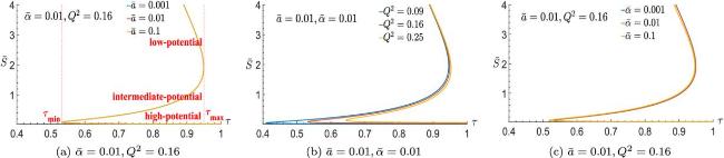
Figure 1. (a)–(c) The zero points of ${\phi }^{\bar{S}}$ in the diagram of $\bar{S}$-τ for the HRN-AdSQ black hole in the canonical ensemble with different values of the parameters $\bar{a}$, $\bar{\alpha }$ and Q2. ($\omega =-\frac{d-2}{d-1},d=4.)$ |
As shown in figure 1, the effects of varying parameters $\bar{a}$, $\bar{\alpha }$ and Q2 on the $\bar{S}-\tau $ curves can be clearly observed. It has been demonstrated that as the charge Q2 in spacetime increases, the interval between high and low potentials concomitantly increases for the same value of τ. Specifically, the region of first-order phase transition is increasing. However, the two parameters $\bar{a}$ and $\bar{\alpha }$ have little effect on $\bar{S}-\tau $ curves.
3.1.2. When d = 4 and ω ≠ − 2/3
From equation (3.4 ), the critical point satisfies the equation as [64]:
$\begin{eqnarray}\begin{array}{l}-1+\frac{3\times 32{\pi }^{2}{\tilde{Q}}^{2}}{8\pi {C}^{2}S}\left(\frac{C}{4}\right)+3S\left(\frac{1}{\pi C}\right)-[2+3\omega ]\frac{3\tilde{\alpha }\omega }{C}{S}^{-\frac{1+3\omega }{2}}{\left(\pi C\right)}^{\frac{1+3\omega }{2}}+\frac{\tilde{a}}{C}=0,\\ \,3-\frac{3\times 5\times 32{\pi }^{2}{\tilde{Q}}^{2}}{8\pi {C}^{2}S}\left(\frac{C}{4}\right)-3S\left(\frac{1}{\pi C}\right)+[2+3\omega ][4+3\omega ]\frac{3\tilde{\alpha }\omega }{C}{S}^{-\frac{1+3\omega }{2}}{\left(\pi C\right)}^{\frac{1+3\omega }{2}}-\frac{3\tilde{a}}{C}=0,\end{array}\end{eqnarray}$
$\begin{eqnarray}\frac{3\pi {\tilde{Q}}^{2}(1-3\omega )}{CS(1+3\omega )}=-\left(1-\frac{\tilde{a}}{C}\right)-\frac{3S}{\pi C}.\end{eqnarray}$
Then, we can obtain:
$\begin{eqnarray}\begin{array}{l}\omega =-\frac{3}{4},{Q}_{c}^{2}=\frac{5{C}^{2}}{12\times 13}{\left(1-\frac{\tilde{a}}{C}\right)}^{2},\,{S}_{c}=\frac{\pi C}{6}\left(1-\frac{\tilde{a}}{C}\right),\\ \omega =-\frac{5}{6},{Q}_{c}^{2}=\frac{{C}^{2}}{28}{\left(1-\frac{\tilde{a}}{C}\right)}^{2},\,{S}_{c}=\frac{\pi C}{6}\left(1-\frac{\tilde{a}}{C}\right).\end{array}\end{eqnarray}$
When $\omega =-\frac{3}{4},\,-\frac{5}{6}$, the critical temperatures are, respectively [65]:
$\begin{eqnarray}{T}_{c}\left(\omega =-\frac{3}{4}\right)=\frac{1}{4\pi L}{\left(\frac{6}{\left(1-\bar{a}\right)}\right)}^{1/2}\left[(1-\bar{a})-\frac{5}{2\times 13}\left(1-\bar{a}\right)+\frac{\left(1-\bar{a}\right)}{2}-\frac{9\bar{\alpha }}{4}{\left(\frac{\left(1-\bar{a}\right)}{6}\right)}^{\frac{5}{8}}\right],\end{eqnarray}$
$\begin{eqnarray}\displaystyle {T}_{c}\left(\omega =-\frac{5}{6}\right)=\frac{1}{4\pi L}{\left(\frac{6}{\left(1-\bar{a}\right)}\right)}^{1/2}\left[\left(1-\bar{a}\right)-\frac{3}{14}\left(1-\bar{a}\right)+\frac{\left(1-\bar{a}\right)}{2}+\,-\frac{5\bar{\alpha }}{2}{\left(\frac{\left(1-\bar{a}\right)}{6}\right)}^{\frac{3}{4}}\right].\end{eqnarray}$
Hence, for ω = $-\frac{3}{4}$, we have
$\begin{eqnarray}\begin{array}{l}t\left(\omega =-\frac{3}{4}\right)=\frac{T}{{T}_{c}}=\frac{{\left(\frac{\pi C}{S}\right)}^{1/2}\left[1-\bar{a}-\frac{4\pi {\tilde{Q}}^{2}}{{C}^{2}}\left(\frac{C}{4S}\right)+3\left(\frac{S}{\pi C}\right)-\frac{9\bar{\alpha }}{4}{\left(\frac{S}{\pi C}\right)}^{\frac{5}{8}}\right]}{{\left(\frac{6}{\left(1-\bar{a}\right)}\right)}^{1/2}\left[1-\bar{a}-\frac{5}{2\times 13}\left(1-\bar{a}\right)+\frac{\left(1-\bar{a}\right)}{2}-\frac{9\bar{\alpha }}{4}{\left(\frac{\left(1-\bar{a}\right)}{6}\right)}^{58}\right]}.\end{array}\end{eqnarray}$
The zero points of ${\phi }^{\bar{S}}$ in the diagram of $\bar{S}-\tau $ with varying parameters $\bar{a}$, $\bar{\alpha }$ and Q2 can be plotted as figure 2 by substituting $\bar{S}{S}_{c}=\bar{S}\frac{\pi C}{6}\left(1-\bar{a}\right)=S$, ${\bar{Q}}^{2}{\tilde{Q}}_{c}^{2}={\bar{Q}}^{2}\frac{5{C}^{2}}{12\times 13}{\left(1-\bar{a}\right)}^{2}={\tilde{Q}}^{2}$ into equation (3.18a ).
Then, for ω = $-\frac{5}{6}$, we have:
$\begin{eqnarray}\displaystyle t\left(\omega =-\frac{5}{6}\right)=\frac{T}{{T}_{c}}=\frac{{\left(\frac{\pi C}{S}\right)}^{1/2}\left[1-\bar{a}-\frac{4\pi {\tilde{Q}}^{2}}{{C}^{2}}\left(\frac{C}{4S}\right)+3\left(\frac{S}{\pi C}\right)-\frac{5\bar{\alpha }}{2}{\left(\frac{S}{\pi C}\right)}^{\frac{3}{4}}\right]}{{\left(\frac{6}{\left(1-\bar{a}\right)}\right)}^{1/2}\left[\left(1-\bar{a}\right)-\frac{3}{14}\left(1-\bar{a}\right)+\frac{\left(1-\bar{a}\right)}{2}+-\frac{5\bar{\alpha }}{2}{\left(\frac{\left(1-\bar{a}\right)}{6}\right)}^{34}\right]}.\end{eqnarray}$
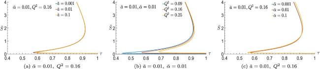
Figure 2. (a)–(c) The zero points of ${\phi }^{\bar{S}}$ in the diagram of $\bar{S}-\tau $ for the HRN-AdSQ black hole in the canonical ensemble with different values of the parameters $\bar{a}$, $\bar{\alpha }$ and Q2. ($d=4,\,\omega =-\frac{3}{4}.)$ |
The zero points of ${\phi }^{\bar{S}}$ in the diagram of $\bar{S}-\tau $ with varying parameters $\bar{a}$, $\bar{\alpha }$ and Q2 can be plotted in figure 3 by substituting $\bar{S}{S}_{c}=\bar{S}\frac{\pi C}{6}\left(1-\bar{a}\right)=S$, ${\bar{Q}}^{2}{\tilde{Q}}_{c}^{2}={\bar{Q}}^{2}\frac{{C}^{2}}{28}{\left(1-\bar{a}\right)}^{2}={\tilde{Q}}^{2}$ into equation (3.18b ).
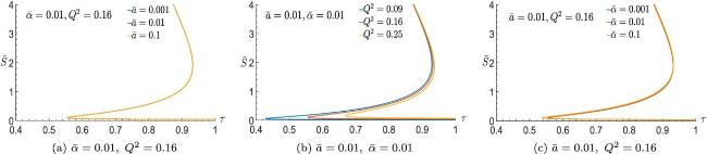
Figure 3. (a)–(c) The zero points of ${\phi }^{\bar{S}}$ in the diagram of $\bar{S}-\tau $ for the HRN-AdSQ black hole in the canonical ensemble with different values of the parameters $\bar{a}$, $\bar{\alpha }$ and Q2. ($d=4,\,\omega =-\frac{5}{6}.)$ |
Furthermore, the zero points of ${\phi }^{\bar{S}}$ in the diagram of $\bar{S}-\tau $ for the HRN-AdSQ black hole in the canonical ensemble are derived as shown in figure 4 with different values of ω and the fixed parameters d = 4, $\bar{a}=0.01$, $\bar{\alpha }=0.01$ and Q2 = 0.16.
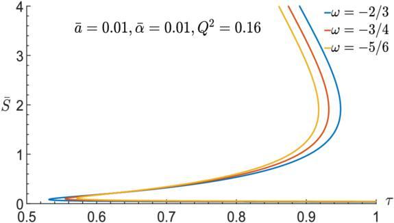
Figure 4. The zero points of ${\phi }^{\bar{S}}$ in the diagram of $\bar{S}$-τ for the HRN-AdSQ black hole in the canonical ensemble with different values of parameter ω. (d = 4, ω=$-\frac{2}{3},-\frac{3}{4},-\frac{5}{6}.$) |
As illustrated in figure 4, the phase transition is shown as a function of ω for the spacetime dimension d = 4, with the specified parameters $\bar{a}$, $\bar{\alpha }$ and Q2. It is evident that the values of ${\tau }_{\max }$ increase, while ${\tau }_{\min }$ decreases in magnitude with increasing ω. Hence, the intervals of ${\tau }_{\min }\lt \tau \lt {\tau }_{\max }$ increase with increasing ω. Specifically, the first-order phase transition interval of the black hole increases with the increase in ω.
3.1.3. When $\omega =-\frac{d-2}{d-1}$ and d = 5, 6
The critical point satisfies the equation: 3.19 ), we can deduce that the critical value is independent of $\bar{\alpha }$. Setting ${\bar{Q}}^{2}={Q}^{2}{y}_{c}\frac{{{\rm{\Omega }}}_{d-2}^{2}}{{\pi }^{2}}$, $\bar{S}={x}_{c}\frac{{{\rm{\Omega }}}_{d-2}}{4}S$, the critical value is obtained in a variety of dimensions d. When $\bar{a}=0$, the critical values for d = 5 are xc = 0.192447; yc = 0.0014, and for d = 6 are xc = 0.202497; yc = 0.0012. Whereas when $\bar{a}$ =0.001, the critical values for d = 5 are xc = 0.192197; yc = 0.0013, and for d = 6 are xc = 0.202197; yc = 9.8215 × 10⁻⁴. The critical temperature Tc of the corresponding parameters can be calculated from the resulting xc and yc. Thus, the zero points of φS in the diagram of S − τ can be plotted for different dimensions d, as shown in figure 5.
$\begin{eqnarray}\begin{array}{l}-(d-3)(3d-7)+(d-1)(d-3)+{\left(\frac{4\bar{S}}{{{\rm{\Omega }}}_{d-2}}\right)}^{2/(d-2)}[(d-1)(3d-7)-(d-1)(d-3)]\\ \,+\,\frac{2\bar{a}}{(d-2)}{\left(\frac{{{\rm{\Omega }}}_{d-2}}{4\bar{S}}\right)}^{\frac{d-4}{(d-2)}}[(d-3)(3d-7)-(d-3)(2d-5)]=0,\\ \,-\,{(d-3)}^{2}+(d-1)(d-2){\left(\frac{4\bar{S}}{{{\rm{\Omega }}}_{d-2}}\right)}^{2/(d-2)}+\bar{a}(d-3){\left(\frac{{{\rm{\Omega }}}_{d-2}}{4\bar{S}}\right)}^{\frac{d-4}{(d-2)}}=0.\end{array}\end{eqnarray}$
From equation (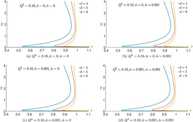
Figure 5. (a)–(d) The zero points of φS in the diagram of S − τ for the HRN-AdSQ black hole in the canonical ensemble with different dimensions d (d = 4, 5, 6). |
As demonstrated in figure 5, the impact of dimension d on the S-τ curve is more pronounced under identical spacetime constraints. Firstly, it is evident that the interval of ${\tau }_{\min }\lt \tau \lt {\tau }_{\max }$ decreases in proportion to the increase in dimension d. Secondly, it is observed that near the annihilation point ($\tau ={\tau }_{\max }$), the value of $\left|\frac{\partial S}{\partial \tau }\right|$ increases as dimension d increases. When $\tau ={\tau }_{\max }-{\rm{\Delta }}\tau $, the increasing dimension d results in an enhancement of the distance between the high and low potentials for a constant Δτ, thereby leading to an expansion of the two-phase coexistence region. Furthermore, it can be demonstrated that the values of $\bar{a}$ and $\bar{\alpha }$ have no effect on the generalization laws of the S − τ curve in the canonical ensemble.
The zero points of the mapping φ can be calculated by φS = 0. In figures 1–5, we can see that there are three states as ${\tau }_{\min }\lt \tau \lt {\tau }_{\max }$; this means the existence of a phase transition in the region of ${\tau }_{\min }\lt \tau \lt {\tau }_{\max }$. The three states are stable (low-potential), unstable (intermediate-potential), and stable (high-potential) black hole states, and the relative winding number is +1, −1, +1, respectively. That is, the topological number of the HRN-AdSQ black hole in a canonical ensemble is always W = +1 −1 + 1 = 1 for the multiple different parameters and higher dimensions. Finally, it is important to note that its topological properties are unaffected by these parameters in a canonical ensemble. These results are consistent with those of RN-AdS black holes [63].
3.2. In the grand canonical ensemble
Now we proceed to investigate the topology of the HRN-AdSQ black hole in the grand canonical ensemble.
3.2.1. When $\omega =-\frac{d-2}{d-1}$ and d = 4
The potential of the black hole is:
$\begin{eqnarray}\displaystyle \tilde{{\rm{\Phi }}}={\left(\frac{\partial M}{\partial \tilde{Q}}\right)}_{S,C,\tilde{\alpha },\tilde{a}}={\left(\frac{C}{4S}\right)}^{(d-3)/(d-2)}\frac{4\pi \tilde{Q}}{{L}^{d-3}C(d-3){{\rm{\Omega }}}_{d-2}^{1/(d-2)}}={\left(\frac{C}{4S}\right)}^{1/2}\frac{2\sqrt{\pi }\tilde{Q}}{LC},\tilde{Q}=\frac{{\rm{\Phi }}LC}{2\sqrt{\pi }}{\left(\frac{4S}{C}\right)}^{1/2},\end{eqnarray}$
when $\begin{eqnarray}\bar{S}{S}_{{\rm{e}}{\rm{x}}{\rm{t}}{\rm{r}}}=\bar{S}\frac{\pi C}{6}\left(1-\frac{\tilde{a}}{C}\right)=S,{\bar{{\rm{\Phi }}}}^{2}{{\rm{\Phi }}}_{{\rm{e}}{\rm{x}}{\rm{t}}{\rm{r}}}^{2}={\bar{{\rm{\Phi }}}}^{2}\frac{\left(1-\bar{a}\right)}{6{L}^{2}}={{\rm{\Phi }}}^{2}.\end{eqnarray}$
Here, ${S}_{{\rm{e}}{\rm{x}}{\rm{t}}{\rm{r}}}=\frac{\pi C}{6}\left(1-\frac{\tilde{a}}{C}\right)$, ${{\rm{\Phi }}}_{{\rm{e}}{\rm{x}}{\rm{t}}{\rm{r}}}^{2}=\frac{\left(1-\bar{a}\right)}{6{L}^{2}}$. Then, the zero points are determined by the expression of φs = 0, so we have: $\begin{eqnarray}\frac{1}{\tau }=\frac{T}{{T}_{c}}=\frac{\left[{(1-\bar{a})}^{1/2}\left(1-\frac{{\bar{{\rm{\Phi }}}}^{2}}{6}+\frac{\bar{S}}{2}\right)-2\bar{\alpha }{\left(\frac{\bar{S}}{6}\right)}^{1/2}\right]}{2{\bar{S}}^{1/2}\left[\frac{2}{3}{\left(1-\bar{a}\right)}^{1/2}-\bar{\alpha }{\left(\frac{1}{6}\right)}^{12}\right]}.\end{eqnarray}$
It is obvious that there is one extreme, when $\bar{S}=2-\frac{{\bar{{\rm{\Phi }}}}^{2}}{3}$, the extreme is: $\begin{eqnarray}\displaystyle {\tau }_{{\rm{e}}{\rm{x}}{\rm{t}}{\rm{r}}}=\frac{2{\bar{S}}^{1/2}\left[\frac{2}{3}{\left(1-\bar{a}\right)}^{1/2}-\bar{\alpha }{\left(\frac{1}{6}\right)}^{\frac{1}{2}}\right]}{\left[{(1-\bar{a})}^{1/2}\left(1-\frac{{\bar{{\rm{\Phi }}}}^{2}}{6}+\frac{\bar{S}}{2}\right)-2\bar{\alpha }{\left(\frac{\bar{S}}{6}\right)}^{1/2}\right]}=\frac{{2}^{3/2}{\left(1-\frac{{\bar{{\rm{\Phi }}}}^{2}}{6}\right)}^{1/2}\left[\frac{2}{3}{\left(1-\bar{a}\right)}^{1/2}-\bar{\alpha }{\left(\frac{1}{6}\right)}^{\frac{1}{2}}\right]}{\left[2{(1-\bar{a})}^{1/2}\left(1-\frac{{\bar{{\rm{\Phi }}}}^{2}}{6}\right)-2\bar{\alpha }{\left(\frac{1}{3}\left(1-\frac{{\bar{{\rm{\Phi }}}}^{2}}{6}\right)\right)}^{1/2}\right]}.\end{eqnarray}$
Thus, the zero points of ${\phi }^{\bar{S}}$ in the diagram of $\bar{S}-\tau $ with varying parameters $\bar{a}$, $\bar{\alpha }$ and ${\overline{{\rm{\Phi }}}}^{2}$ in the grand ensemble are displayed in figure 6. Here, τextr is related to the annihilation point. As τ < τextr, there are two intersection points for the HRN-AdSQ black hole in the grand canonical ensemble. They correspond to the stable (low-potential) and unstable (high-potential) black hole states, respectively, as demonstrated in Du’s article [62]. The corresponding winding numbers are +1 and −1; therefore, the topological number when $\omega =-\frac{d-2}{d-1}$ and d = 4 is W = 1 − 1 = 0 as τ < τextr. For τ = τextr, the two intersection points for the HRN-AdSQ black hole coincide. Furthermore, there is no black hole as τ > τextr.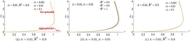
Figure 6. (a)–(b) The zero points of ${\phi }^{\bar{S}}$ in the diagram of $\bar{S}$-τ for the HRN-AdSQ black hole in the grand canonical ensemble with different values of the parameters $\bar{a}$, $\bar{\alpha }$ and ${\overline{{\rm{\Phi }}}}^{2}$. ($d=4,\,\omega =-\frac{d-2}{d-1}.)$ |
As illustrated in figure 6, the impact of parameters $\bar{a}$, $\bar{\alpha }$ and ${\overline{{\rm{\Phi }}}}^{2}$ on the zero points of φS in the diagram of $\bar{S}-\tau $ for the grand canonical ensemble appears to be analogous to their effects in the canonical ensemble.
3.2.2. When d = 4 and ω ≠ − 2/3
From equation (3.4 ), the critical point τ = τextr satisfies the equation:
$\begin{eqnarray}\begin{array}{l}\omega =-\frac{3}{4},{\tilde{Q}}_{{\rm{e}}{\rm{x}}{\rm{t}}{\rm{r}}}^{2}=\frac{5{C}^{2}}{12\times 13}{\left(1-\frac{\tilde{a}}{C}\right)}^{2},{S}_{{\rm{e}}{\rm{x}}{\rm{t}}{\rm{r}}}=\frac{\pi C}{6}\left(1-\frac{\tilde{a}}{C}\right),\,{\tilde{{\rm{\Phi }}}}_{{\rm{e}}{\rm{x}}{\rm{t}}{\rm{r}}}^{2}=\frac{15}{13\times 6{L}^{2}}\left(1-\frac{\tilde{a}}{C}\right),\\ \omega =-\frac{5}{6},{\tilde{Q}}_{{\rm{e}}{\rm{x}}{\rm{t}}{\rm{r}}}^{2}=\frac{{C}^{2}}{28}{\left(1-\frac{\tilde{a}}{C}\right)}^{2},{S}_{{\rm{e}}{\rm{x}}{\rm{t}}{\rm{r}}}=\frac{\pi C}{6}\left(1-\frac{\tilde{a}}{C}\right),\,{{\rm{\Phi }}}_{{\rm{e}}{\rm{x}}{\rm{t}}{\rm{r}}}^{2}=\frac{3}{14{L}^{2}}\left(1-\frac{\tilde{a}}{C}\right).\end{array}\end{eqnarray}$
When ω = $-\frac{3}{4},\,-\frac{5}{6}$, the temperatures at the critical points τ = τextr are, respectively: $\begin{eqnarray}\begin{array}{l}{T}_{{\rm{e}}{\rm{x}}{\rm{t}}{\rm{r}}}(\omega =-\frac{3}{4})=\frac{1}{4\pi L}{\left(\frac{6}{\left(1-\bar{a}\right)}\right)}^{1/2}\left[1-\bar{a}-\frac{5}{2\times 13}\left(1-\bar{a}\right)+\frac{\left(1-\bar{a}\right)}{2}-\frac{9\bar{\alpha }}{4}{\left(\frac{\left(1-\bar{a}\right)}{6}\right)}^{\frac{5}{8}}\right],\\ {T}_{{\rm{e}}{\rm{x}}{\rm{t}}{\rm{r}}}(\omega =-\frac{5}{6})=\frac{1}{4\pi L}{\left(\frac{6}{\left(1-\bar{a}\right)}\right)}^{1/2}\left[\left(1-\bar{a}\right)-\frac{3}{14}\left(1-\bar{a}\right)+\frac{\left(1-\bar{a}\right)}{2}+-\frac{5\bar{\alpha }}{2}{\left(\frac{\left(1-\bar{a}\right)}{6}\right)}^{\frac{3}{4}}\right].\end{array}\end{eqnarray}$
Hence, for ω = −$\frac{3}{4}$, we have:
$\begin{eqnarray}\displaystyle t\left(\omega =-\frac{3}{4}\right)=\frac{T}{{T}_{{\rm{extr}}}}=\frac{{\left(\frac{\pi C}{S}\right)}^{1/2}\left[1-\bar{a}-\frac{4\pi {\tilde{Q}}^{2}}{{C}^{2}}\left(\frac{C}{4S}\right)+3\left(\frac{S}{\pi C}\right)-\frac{9\bar{\alpha }}{4}{\left(\frac{S}{\pi C}\right)}^{\frac{5}{8}}\right]}{{\left(\frac{6}{\left(1-\bar{a}\right)}\right)}^{1/2}\left[1-\bar{a}-\frac{5}{2\times 13}\left(1-\bar{a}\right)+\frac{\left(1-\bar{a}\right)}{2}-\frac{9\bar{\alpha }}{4}{\left(\frac{\left(1-\bar{a}\right)}{6}\right)}^{58}\right]}.\end{eqnarray}$
The zero points of ${\phi }^{\bar{S}}$ in the diagram of $\bar{S}-\tau $ with varying parameters $\bar{a}$, $\bar{\alpha }$ and ${\overline{{\rm{\Phi }}}}^{2}$ can be plotted as shown in figure 7 by substituting $\bar{S}{S}_{{\rm{e}}{\rm{x}}{\rm{t}}{\rm{r}}}=\bar{S}\frac{\pi C}{6}\left(1-\bar{a}\right)=S$, ${\bar{{\rm{\Phi }}}}^{2}{{\rm{\Phi }}}_{{\rm{e}}{\rm{x}}{\rm{t}}{\rm{r}}}^{2}={\bar{{\rm{\Phi }}}}^{2}\frac{15}{13\times 6{L}^{2}}\left(1-\bar{a}\right)={{\rm{\Phi }}}^{2}$ into equation (3.26a ).
Then, for ω = −$\frac{5}{6}$, we have:
$\begin{eqnarray}t\left(\omega =-\frac{5}{6}\right)=\frac{T}{{T}_{{\rm{extr}}}}=\frac{{\left(\frac{\pi C}{S}\right)}^{1/2}\left[1-\bar{a}-\frac{4\pi {\tilde{Q}}^{2}}{{C}^{2}}\left(\frac{C}{4S}\right)+3\left(\frac{S}{\pi C}\right)-\frac{5\bar{\alpha }}{2}{\left(\frac{S}{\pi C}\right)}^{\frac{3}{4}}\right]}{{\left(\frac{6}{\left(1-\bar{a}\right)}\right)}^{1/2}\left[\left(1-\bar{a}\right)-\frac{3}{14}\left(1-\bar{a}\right)+\frac{\left(1-\bar{a}\right)}{2}+-\frac{5\bar{\alpha }}{2}{\left(\frac{\left(1-\bar{a}\right)}{6}\right)}^{34}\right]}.\end{eqnarray}$
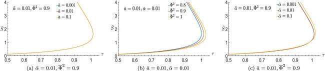
Figure 7. (a)–(c) The zero points of ${\phi }^{\bar{S}}$ in the diagram of $\bar{S}$-τ for the HRN-AdSQ black hole in the grand canonical ensemble with different values of the parameters $\bar{a}$, $\bar{\alpha }$ and ${\overline{{\rm{\Phi }}}}^{2}$. (d = 4, $\omega =-\frac{3}{4}.)$ |
The zero points of ${\phi }^{\bar{S}}$ in the diagram of $\bar{S}-\tau $ with varying parameters $\bar{a}$, $\bar{\alpha }$ and ${\overline{{\rm{\Phi }}}}^{2}$ can be plotted as shown in figure 8 by substituting $\bar{S}{S}_{{\rm{e}}{\rm{x}}{\rm{t}}{\rm{r}}}=\bar{S}\frac{\pi C}{6}\left(1-\bar{a}\right)=S$, ${\bar{{\rm{\Phi }}}}^{2}{{\rm{\Phi }}}_{{\rm{e}}{\rm{x}}{\rm{t}}{\rm{r}}}^{2}={\bar{{\rm{\Phi }}}}^{2}\frac{3}{14{L}^{2}}\left(1-\bar{a}\right)={{\rm{\Phi }}}^{2}$ into equation (3.26b ).
Figure 8. (a)–(c) The zero points of ${\phi }^{\bar{S}}$ in the diagram of $\bar{S}$-τ for the HRN-AdSQ black hole in the grand canonical ensemble with different values of the parameters $\bar{a}$, $\bar{\alpha }$ and ${\overline{{\rm{\Phi }}}}^{2}$. ($d=4,\,\omega =-\frac{5}{6}.)$ |
To conclude, the zero points of ${\phi }^{\bar{S}}$ in the diagram of $\bar{S}-\tau $ for the HRN-AdSQ black hole in the grand canonical ensemble are plotted as shown in figure 9 for varying values of ω, while maintaining fixed values of d = 4, $\bar{a}=0.01$, $\bar{\alpha }=0.01$ and ${\overline{{\rm{\Phi }}}}^{2}=0.9$.
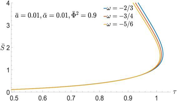
Figure 9. The zero points of ${\phi }^{\bar{S}}$ in the diagram of $\bar{S}$-τ for the HRN-AdSQ black hole in the grand canonical ensemble with different values of parameter ω (d = 4, $\omega =-\frac{2}{3},-\frac{3}{4},-\frac{5}{6}$). |
As illustrated in figure 9, the zero points of ${\phi }^{\bar{S}}$ in the diagram of $\bar{S}-\tau $ for the HRN-AdSQ black hole in the grand canonical ensemble are shown as a function of ω for the spacetime dimension d = 4, with specified parameters $\bar{a}$, $\bar{\alpha }$ and ${\overline{{\rm{\Phi }}}}^{2}$. It is evident that the values of τextr decrease with the decreasing ω.
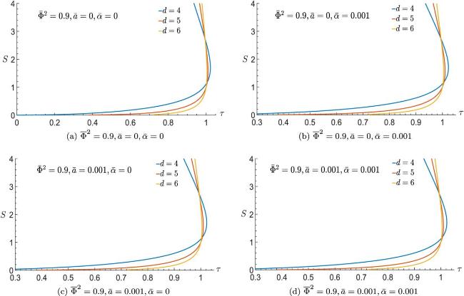
3.2.3. When $\omega =-\frac{d-2}{d-1}$ and d = 5, 6
According to equation (3.3 ), when $\bar{S}=x\frac{{{\rm{\Omega }}}_{d-2}}{4}$, ${\bar{Q}}^{2}={{\rm{\Phi }}}^{2}\frac{{L}^{2}\bar{S}}{\pi }$, ${{\rm{\Phi }}}_{{\rm{e}}{\rm{x}}{\rm{t}}{\rm{r}}}^{2}={y}_{{\rm{e}}{\rm{x}}{\rm{t}}{\rm{r}}}\frac{{{\rm{\Omega }}}_{d-2}}{{L}^{2}}$, as is also the case with the analytical methods in the canonical ensemble. When $\bar{a}=0$, the critical values for d = 5 are xextr = 0.192447; yextr = 0.0092, and for d = 6 are xextr = 0.202497; yextr = 0.0077. Whereas when $\bar{a}=0.001$, the critical values for d = 5 are xextr = 0.192197; yextr = 0.0092, and for d = 6 are xextr = 0.202197; yextr = 0.0077. Setting ${\bar{{\rm{\Phi }}}}^{2}={y}_{{\rm{e}}{\rm{x}}{\rm{t}}{\rm{r}}}\frac{{{\rm{\Omega }}}_{d-2}}{{L}^{2}}{{\rm{\Phi }}}^{2}$, $\bar{S}={x}_{{\rm{extr}}}\frac{{{\rm{\Omega }}}_{d-2}}{4}S$, then the zero points of φS in the diagram of S-τ can be plotted for different $\bar{a}$, $\bar{\alpha }$ and d, as shown in figure 10.
Figure 10. (a)–(d) The zero points of φS in the diagram of S − τ for the HRN-AdSQ black hole in the grand canonical ensemble with different dimensions d (d = 4, 5, 6). |
The zero points of ${\phi }^{\bar{S}}$ in the diagram of $\bar{S}-\tau $(S-τ) in the grand canonical ensemble with multiple related parameters, including $\bar{a}$, $\bar{\alpha }$, ${\overline{{\rm{\Phi }}}}^{2}$, ω and dimension d, are displayed in figures 6–10. As demonstrated in these figures, it is evident that all the specified parameters exert an influence on the $\bar{S}-\tau $(S-τ) curve in the grand canonical ensemble. However, there are always two states, including stable (low-potential) and unstable (high-potential) black hole states; as τ < τextr, the corresponding winding numbers are +1 and −1, respectively. Specifically, the topological number of the HRN-AdSQ black hole in the grand canonical ensemble is always W = 1−1 = 0 for the multiple different parameters and higher dimensions. And most importantly, its topological properties are unaffected by these parameters in the grand canonical ensemble.
4. Discussion and conclusions
In this work, under the restricted phase space frame we investigated the thermodynamical topology of the HRN-AdSQ black hole. We analyzed the effects of varying parameters of spacetime and the higher dimension d on the zero points of ${\phi }^{\bar{S}}$ in the diagram of $\bar{S}-\tau \,(S-\tau $). As demonstrated in section 3 , the multiple spacetime parameters have an influence on the $\bar{S}-\tau \,(S-\tau $) curve; however, they do not exert an influence on the topological number of the spacetime. In addition, the dimension d has no effect on the topology. It can thus be concluded that these topological numbers are universal constants that are independent of the specific parameters of black holes. It is imperative to acknowledge their significance in elucidating the fundamental nature of black holes and gravity. Furthermore, these observations may provide new insights for the development of quantum gravity theory. It is important to acknowledge that the topological number of a black hole is contingent on the external environment in which it is located. That is, the environment is the canonical ensemble of only energy exchange between the black hole and the outside world, or the grand canonical ensemble of both energy exchange and particle exchange between the black hole and the outside world. Specifically, when classifying the thermodynamic properties of black holes according to the topological number, it is necessary to take into account the external environment in which the spacetime is located.