


1. Introduction
Signaling networks incessantly carry out information transmission between cells and the outside world through a series of biochemical pathways, such as enzymatic cascade, gene expression networks, etc [1, 2]. Biochemical reaction networks are usually described with deterministic rate equations and the state of the network is accessed through solving ordinary differential equations (ODEs). This type of description is based on mass action law and valid only when the numbers of reactants are big enough. However, the signaling dynamics is usually highly stochastic [3–6] due to the small numbers of molecules involved in biochemical reactions in a cell. One extreme example is the gene expression where there is only one DNA. Therefore, it is important to study the impact of randomness in cell signaling [3, 5–7], where stochasticity may have an impact on cell size, cell cycle, or anomalies in cell signaling pathways [8–11].
One popular mesoscopic model describing randomness is the chemical master equation (CME), which is a set of ODEs that govern the time evolution of the probability distribution, based on the Markovian assumption and able to accurately characterize the intrinsic randomness of the system. Different numerical or analytical approaches are developed to solve these CMEs. However, the state space dimension of the CME grows exponentially with the number of molecular species, making it infeasible to directly approach high-dimensional systems.
As a result, many numerical algorithms are designed to simulate the stochastic dynamics, the most widely used of which is the Gillespie algorithm [12, 13]. It is an accurate Monte Carlo computation scheme that generates statistically exact trajectories of the CME by sampling each reaction that takes place during the time interval under investigation, which is nevertheless computationally expensive especially for systems with many molecules or large span of time scales. Later development involves various extensions of the algorithm: the tau-leaping algorithm [14], which employs Poisson random numbers to batch multiple reaction events to one step to accelerate the simulation. However, an improper selection of the time step in tau-leaping may lead to negative molecular number (negative population problem). Also, in pathways with very different reaction rates, the computation could become inefficient due to the notoriously well-known stiffness problem. To cope with these caveats, Cao et al proposed improved algorithms for tau-leaping, with optimized stepsize selection schemes [15–19] or the quasi-equilibrium assumptions [20–23]. The explicit, the implicit, or the adaptive tau-selection algorithms [15, 17] did a good job in stepsize selection but unfortunately with much increased computational complexity; the binomial tau-leaping replaces the Poisson distribution with a binomial one to avoid negative numbers [24, 25], but also results in high computational cost. Tang [26] proposed a machine learning scheme using variational autoregressive networks and show flexibility in representing multi-modal distributions but its efficiency needs further investigation.
On the other hand, a clever exploitation of the analytical structure of stochastic dynamics may significantly accelerate its computation and better reveal the underlying principles of cell operation in different conditions [27, 28]. To challenge the dimensionality curse encountered in solving the CME with many molecules, methods such as moment closure or binomial moments [29–33] are designed, which reduce high-dimensional CMEs to a system of ODEs satisfied by low-order moments with the high-order ones being truncated, significantly lowering computational load. However, their performance is highly dependent on factors such as the system’s nonlinearity or complexity of distribution profiles. Therefore, careful selection of truncation schemes is required for a specific system. The generating function method is also employed to transform a large set of CMEs [27, 28, 34] to one partial differential equation (PDE), but its application in the biochemical reaction network is limited due to the difficulty of directly solving PDEs with multiple independent variables. In fact, variational methods [5, 35, 36] were proposed to solve these PDEs but succeeded only in reaction networks with simple molecular distributions.
The key of a successful application of the variational method is the selection of the variational basis functions, including the right basis, which should well capture the probability distribution and the left basis, which provides observable statistical indicators to characterize the distribution. Huang [36] proposed alternative right basis functions to better capture multi-peak distributions in several typical biochemical reaction networks but a systematic approach was still lacking in general situations. Recently, Cai [37] made further improvement and delivered empirical guidelines for constructing the right basis, which is expected to play a role in a wide range of cell signaling networks. However, in all the above approaches, the left basis is a linear combination of differential operators, so high-order derivatives may result when dealing with complex multimodal distributions whose description requires a large number of time-varying parameters, which may greatly decrease the efficiency and even undermine the computation accuracy. To cope with this problem, in the current paper,based on the Fourier analysis and Gaussian distribution, a new selection of the left basis is proposed, which is good at depicting the multimodal or highly localized distributions. A combined utilization of these left basis functions greatly improves the efficiency, which revives the variational approach as a versatile and powerful tool for analyzing the molecular behavior and reaction mechanism in a cell.
In the following, section 2 briefly explains the variational approach of the CME in a generating function formulation. A variational functional is discussed with the setup of test wave functions. In section 3 , three different selections of observables are introduced in sequel including the conventional one based on moments, and our new design involving the Fourier basis and the Gaussian distributions. In section 4 , four classical biochemical reaction models of cell signaling pathways are used to demonstrate the effectiveness of the new scheme. We conclude the article and point out interesting future directions in section 5 .
2. The variational treatment of chemical master equation
In an interesting analogy with the wave function in quantum mechanics [38, 39], the dynamically changing probability distribution in the state space provides a fundamental characterization of the biochemical reaction system. It is possible to describe the evolution of the probability distribution with a variational scheme as is popularly exercised in diverse fields involving the solution of complex wave equations [5, 40, 41]. For example, Eyink [40] developed a variational method that provides an effective approximation for turbulent energy fluctuations. Sasai and Wolynes [5, 41] innovatively applied quantum field theory to model the randomness in gene expression, and effectively handled the dynamics of gene networks with a variational technique. This approach transforms complex many-body evolution equations into a set of finite set of ODEs which enables a description with a few parameters and thus greatly simplifies the computation procedure. Below, a detailed explanation of this framework in a generating function formalism is given starting from an introduction of the CME.
2.1. Chemical master equation and generating function formalism
Biochemical reaction is essentially random, which may mathematically be regarded as a Markov process in the state space. In the CME, the system is typically modeled as a collection of discrete states representing the number of molecules of each species involved in the reaction network and the master equation characterizes the change of states in time with a probability description.
For n molecular species involved in R chemical reactions, the general form of the CME is 1 ) is a set of linear equations defined on the set of all accessible states of the system through the R reactions, which could be a very large set and thus pose considerable difficulty in its solution.
$\begin{eqnarray}\begin{array}{rcl}\frac{{\rm{d}}P({\boldsymbol{m}},t)}{{\rm{d}}t} & = & \displaystyle \sum _{j=1}^{R}{a}_{j}({\boldsymbol{m}}-{w}_{j})P({\boldsymbol{m}}-{w}_{j},t)\\ & & -\displaystyle \sum _{j=1}^{R}{a}_{j}({\boldsymbol{m}})P({\boldsymbol{m}},t),\end{array}\end{eqnarray}$
where ${\boldsymbol{m}}={({m}_{1},{m}_{2},\,\ldots ,\,{m}_{n})}^{t}$ represents the state of the system and P(m, t) is the probability distribution at time t. The variable mi is the molecule number of the ith species and aj is the propensity function for the jth reaction with its stoichiometric coefficients being wj. Equation (As an example, the Schlogl model [42, 43] is a typical biochemical bistable system: ${B}_{1}+2X\mathop{\mathop{\rightleftharpoons }\limits_{{c}_{2}}}\limits^{{c}_{1}}3X$, ${B}_{2}\mathop{\mathop{\rightleftharpoons }\limits_{{c}_{4}}}\limits^{{c}_{3}}X$ with four reaction rates ${\{{c}_{i}\}}_{i=1,2,3,4}$. In many applications, the numbers N1, N2 of reactants B1, B2 are assumed to be constant and the number m of X marks the state of the system. The probability distribution P(m) satisfies the following CME
$\begin{eqnarray}\begin{array}{rcl}\frac{{\rm{d}}P(m)}{{\rm{d}}t} & = & \frac{{c}_{1}{N}_{1}}{2}[(m-1)(m-2)P(m-1)\\ & & -\,m(m-1)P(m)]\\ & & +\,\frac{{c}_{2}}{6}[(m+1)m(m-1)P(m+1)\\ & & -\,m(m-1)(m-2)P(m)]\\ & & +\,{c}_{3}{N}_{2}[P(m-1)-P(m)]\\ & & +\,{c}_{4}[(m+1)P(m+1)-mP(m)],\end{array}\end{eqnarray}$
the solution of which provides all the necessary information to analyze the signaling dynamics. Nevertheless, for each possible state m, there is a dynamical variable P(m) and an equation for it. Hence, there involve a large number of ordinary differential equations if the reactions lead to large quantity of X’s. In this case, though, the reaction topology is quite simple: the dynamics of P(m) depends only on its closest neighbors P(m + 1) and P(m − 1). To compactify this type of information and make it amenable to analytic approximation, we introduce the generating function $\begin{eqnarray}{{\rm{\Psi }}}_{R}(x)=\displaystyle \sum _{m=0}^{\infty }P(m){x}^{m},\end{eqnarray}$
which encodes all the information contained in the probability density P(m). Here, x is a formal variable for the reactant X. For example, by evaluating the function or its derivatives at x = 1, the probability conservation, the first and second moments of the reactant X are conveniently expressed $\begin{eqnarray}\begin{array}{rcl}{{\rm{\Psi }}}_{R}(1) & = & 1,\\ \langle m\rangle & = & \frac{\partial {{\rm{\Psi }}}_{R}}{\partial x}{| }_{x=1},\\ \langle {m}^{2}\rangle & = & \left(\frac{{\partial }^{2}{{\rm{\Psi }}}_{R}}{\partial {x}^{2}}+\frac{\partial {{\rm{\Psi }}}_{R}}{\partial x}\right){| }_{x=1}.\end{array}\end{eqnarray}$
Alternatively, the CME turns to a PDE satisfied by the generating function 2 )) specifically, equation (5 ) is
$\begin{eqnarray}\frac{\partial {{\rm{\Psi }}}_{R}}{\partial t}-{\rm{\Omega }}{{\rm{\Psi }}}_{R}=0,\end{eqnarray}$
where Ω is a linear operator derived from the master equation. For the Schlogl model (equation ( $\begin{eqnarray}\begin{array}{rcl}\frac{\partial {{\rm{\Psi }}}_{R}}{\partial t} & = & ({x}^{3}-{x}^{2})\left(\frac{{c}_{1}{N}_{1}}{2}\frac{{\partial }^{2}}{\partial {x}^{2}}-\frac{{c}_{2}}{6}\frac{{\partial }^{3}}{\partial {x}^{3}}\right){{\rm{\Psi }}}_{R}\\ & & +\,(x-1)\left({N}_{2}{c}_{3}-{c}_{4}\frac{\partial }{\partial x}\right){{\rm{\Psi }}}_{R}.\end{array}\end{eqnarray}$
2.2. The variational function
In order to solve equation (5 ), a variational approach is employed by Eyink [40], Sasai [5, 41] by proposing the following variation functional
$\begin{eqnarray}H[{{\rm{\Psi }}}_{L},{{\rm{\Psi }}}_{R}]={\int }_{0}^{\infty }{\rm{d}}t\left\langle {{\rm{\Psi }}}_{L}| \partial t-{\rm{\Omega }}| {{\rm{\Psi }}}_{R}\right\rangle ,\end{eqnarray}$
where the right test function $\Psi$R = $\Psi$R(x, fi(t)) describes the system state and the left test function ${{\rm{\Psi }}}_{L}={{\rm{\Psi }}}_{L}(\frac{{\rm{d}}}{{\rm{d}}x},{v}_{i}(t))$ represents the conjugate observables. Here, the time-dependent parameters {fi(t)} characterize the distribution and the parameters {vi(t)} are variational coefficients, which give the evolution of {fi(t)} based on the variational principle—minimization of H[$\Psi$L, $\Psi$R].2.3. Construction of the wave functions
The wave function $\Psi$R describes the probability distribution and needs to satisfy the following constraints:
(1) It must satisfy the probability conservation condition, which is the first equation in equation (4 ).
(2) The probability distribution must be positive, meaning that the coefficients of the Taylor series of $\Psi$R at x = 0 should be all non-negative.
(3) According to the variational principle, the evolution equation of the time-dependent parameters {fi(t)} in the wave functions can be conveniently obtained by selecting appropriate left test functions.
In biochemical reaction systems, the simplest one is the linear system, through the analysis of which, we can obtain the exact solution of equation (5 ) with methods of characteristics. The general form of the solution consists in polynomials or exponentials and provides an important reference for us to deal with also nonlinear systems [34, 35, 44].
However, due to the frequent appearance of multiple peaks or skewed distribution profiles in higher-order reactions, multi-nomial or Poisson distributions are not sufficient. Therefore, in a previous article [37], a general form of the right basis function is proposed, which considers the reaction topology and is very flexible in dealing various types of distributions. In the current paper, alternative choices of left observables are introduced and explained such that the variational formalism could be applied to reaction networks with medium or large sizes and with complex probability distributions.
3. Alternative choices of observables
Although only a very low-dimensional subspace is enough to accommodate the function $\Psi$R [36], we still need to find appropriate observables $\Psi$L to determine the evolution of all the parameters {fi(t)}. A good choice of $\Psi$L plays the role of an observer trying to seek and emphasize important features of the actual distribution. In the literature [5, 41], different moments are used, to be explained below. However, as the complexity of the model increases, the number of the parameters {fi(t)} rises sharply. Alternative observable functions need to be designed.
3.1. Observables based on moments
For the cost function equation (7 ), $\Psi$L in Sasai et al [5, 41] is actually a polynomial of differential operators
$\begin{eqnarray}{{\rm{\Psi }}}_{L}=1+\displaystyle \sum _{i=1}^{k}{v}_{i}(t){\left(\frac{{\rm{d}}}{{\rm{d}}x}\right)}^{i},\end{eqnarray}$
where k is the chosen order, being closely related to the number of fi’s. The minimization condition of H($\Psi$L, $\Psi$R) corresponds to $\begin{eqnarray}\frac{{{\rm{d}}}^{i}}{{\rm{d}}{x}^{i}}(\partial t-{\rm{\Omega }}){{\rm{\Psi }}}_{R}{| }_{x=1}=0,i=1,2,3...k,\end{eqnarray}$
indicating that the first k derivatives are all zero in the Taylor expansion around x = 1. Therefore, in the limit k → ∞, the equation ∂t$\Psi$R = Ω$\Psi$R holds identically. If k is finite, this equation becomes approximate which determines the evolution of the parameters {fi}.A close look may be taken to see how this condition is related to the projection to the system’s moments. When we take derivatives of a function $\Psi$R, different polynomials of m results as shown below
$\begin{eqnarray}\begin{array}{rcl}\partial x{{\rm{\Psi }}}_{R} & = & \displaystyle \sum _{m=0}^{\infty }mP(m){x}^{m-1},\\ \partial xx{{\rm{\Psi }}}_{R} & = & \displaystyle \sum _{m=0}^{\infty }m(m-1)P(m){x}^{m-2}.\end{array}\end{eqnarray}$
At x = 1, the above two expressions turn to inner products of these polynomials with the distribution P(m), or alternatively represent projections of P to polynomial basis. Obviously, the first derivative is related to the first moment while the second derivative to a combination of the first and the second moment. Therefore, the condition equation (9 ) requires the vanishment of the low-order moments, which is similar to the Galerkin truncation [45] in numerical PDEs.
Different observables exhibit different characteristics [30, 32, 33]. For example, we may choose to expand at x = 0. For the generating function $\Psi$R(x, t) = f0 + f1x + f2x2 + f3x3..., we have 10 ) has a shrinking factor (0.5)m. When m is large, the weight will be very small, which is thus suitable for describing probability distributions near x = 0.
$\begin{eqnarray}\begin{array}{l}\partial x{{\rm{\Psi }}}_{R}{| }_{x=0}={f}_{1},\\ \frac{1}{2}\partial xx{{\rm{\Psi }}}_{R}{| }_{x=0}={f}_{2},\\ \frac{1}{6}\partial xxx{{\rm{\Psi }}}_{R}{| }_{x=0}={f}_{3},\end{array}\end{eqnarray}$
where the probabilities at m = 1, 2, 3 are obtained, as shown in figure 1, where the horizontal axis NX represents the number of molecules and the vertical axis P(NX) represents the probability. So the expansion at x = 0 seems to produce delta-function like test functions, which describe individual probabilities instead of moments. It is also possible to expand at other x values [32, 33], say at x = 0.5, for which a decaying profile is obtained since now each term of the m-polynomial in equation (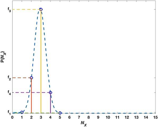
Figure 1. Probability distribution near the origin. |
The above choices of the left observable functions are widely used and quite effective for simple reaction pathways. However, we find two disadvantages popping up in practice. First, no matter around which value of x the generating function is expanded, we have to take as many derivatives as the number of the time-dependent parameters {fi}. For multi-peaked distributions, quite a few such parameters may be needed to describe $\Psi$R while taking many derivatives may lead to enormous number of terms and excessively large numerical values in the expression. Second, in the current scheme with moments, it is not straightforward to map out complex distributions, especially in the presence of multiple molecular species, even when $\Psi$R is properly given. These two difficulties make up one major obstacle for extensive application of the variational approach. In the following sections, we design alternative forms of $\Psi$L that relieve much of the trouble.
3.2. Fourier basis functions
To capture multi-modal distributions, polynomials may not be a good choice for $\Psi$L. For example, a multi-nomial distribution has a very rigid profile: one peak and with the main axis of the level set aligning along the coordinate axis. Instead, Fourier series excels at depicting oscillatory behaviors. With this thought, in the generating function, we put x = eiθ to reach a Fourier transform of the distribution P(m) 14 ) has two terms Explicitly, for the first term, ${\mu }_{1}\,=M({f}_{1}-{f}_{2}+{f}_{1}{f}_{2}),{\sigma }_{1}=M(1+{f}_{2})({f}_{1}-{f}_{1}^{2})$ and for the second term ${\mu }_{2}=M({f}_{3}-{f}_{4}+{f}_{3}{f}_{4}),{\sigma }_{2}=M(1+{f}_{4})({f}_{3}\,-{f}_{3}^{2})$. Many length scales may be invoked for complex distributions.
$\begin{eqnarray}{{\rm{\Psi }}}_{R}({{\rm{e}}}^{{\rm{i}}\theta })=\displaystyle \sum _{m=0}^{M}P(m){{\rm{e}}}^{{\rm{i}}\theta m},\end{eqnarray}$
where M is the maximal number of molecules and θ = 2π/χ is the fundamental frequency with χ usually being a statistical indicator of the sought distribution. In this frame of formulation, we have substantially more choices to extract information from $\Psi$R(x, {fi}) since now x takes values on the unit circle in the complex plane at which the evolution equation (∂t − Ω)$\Psi$R = 0 should identically hold. In the current formulation, $\Psi$R is an approximation with finitely many time-dependent parameters {fi(t)}. For each term in the given expression of $\Psi$R, it is convenient to compute the average position μ and the width σ corresponding to the distribution represented by this term. One convenient choice of χ is χ = μ or χ = σ. For example, in the Schlogl model below, the $\Psi$R given in equation (In this way, we project the probability distribution function into Fourier series containing the position or the width information, and the minimization condition becomes
$\begin{eqnarray}\left(\frac{\partial {{\rm{\Psi }}}_{R}}{\partial t}-{\rm{\Omega }}{{\rm{\Psi }}}_{R}\right){| }_{x={{\rm{e}}}^{{\rm{i}}\theta }}=0,\end{eqnarray}$
which eliminates the need for taking derivatives and thus greatly reduces the computational complexity. Moreover, the above equation may give two real-valued equations since its real and imaginary part should both be zero.As an example, in the Schlogl model mentioned in section 2.1 , if the right test function is selected as
$\begin{eqnarray}\begin{array}{rcl}{{\rm{\Psi }}}_{R}(x,t) & = & {f}_{5}{(1+{f}_{1}(x-1))}^{M+M{f}_{2}}{x}^{-M{f}_{2}}\\ & & +\,(1-{f}_{5}){(1+{f}_{3}(x-1))}^{M+M{f}_{4}}{x}^{-M{f}_{4}},\end{array}\end{eqnarray}$
which contains five time-dependent parameters ${\{{f}_{i}\}}_{i=1,2,3,4,5}$ with M being the maximal number of the reactant X. Here, two terms are present in $\Psi$R since there are two stable fixed points in the corresponding deterministic equation which lead to two Gaussian-like modes. In principle, more terms could be used but they produce similar results. For simplicity, here, we use minimal number of terms.The left test function could be selected as a linear combination of differential operators as usual [5, 41]14 ) as discussed above. The detailed parameter values and numerical results are relegated to section 4.1 .
$\begin{eqnarray}{{\rm{\Psi }}}_{L}={v}_{1}\partial x+{v}_{2}\partial xx+{v}_{3}\partial xxx+{v}_{4}\partial xxxx+{v}_{5}\partial xxxxx,\end{eqnarray}$
where a fifth-order derivative has to be taken to match the number of unknown parameters. If M ∼ 105, a factor of order 1025 will be multiplied after taking the fifth-order derivative, which may devastate the accuracy of the whole computation. If Fourier basis is used instead, higher derivatives are not needed. The condition may be written as $\begin{eqnarray}\begin{array}{rcl}{\partial }_{x}\left(\frac{\partial {{\rm{\Psi }}}_{R}}{\partial t}-{\rm{\Omega }}{{\rm{\Psi }}}_{R}\right){| }_{x=1} & = & 0,\\ \left(\frac{\partial {{\rm{\Psi }}}_{R}}{\partial t}-{\rm{\Omega }}{{\rm{\Psi }}}_{R}\right){| }_{x={{\rm{e}}}^{({\rm{i}}{\theta }_{1})}} & = & 0,\\ \left(\frac{\partial {{\rm{\Psi }}}_{R}}{\partial t}-{\rm{\Omega }}{{\rm{\Psi }}}_{R}\right){| }_{x={{\rm{e}}}^{({\rm{i}}{\theta }_{2})}} & = & 0,\end{array}\end{eqnarray}$
where ${\theta }_{1}=\frac{2\pi }{{\mu }_{1}}$, ${\theta }_{2}=\frac{2\pi }{{\mu }_{2}}$ with μ1, μ2 are the averages corresponding to the distributions of the first and the second term in equation (The time evolution {dfi/dt} has to be computed from equation (16 ). In practice, a numerical matrix inversion is employed by writing equation (16 ) in a matrix form 16 ) are complex, they actually contain four real equations, which together with the first determine the time evolution for the five time-dependent parameters.
$\begin{eqnarray}T\frac{{\rm{d}}f}{{\rm{d}}t}=H,\end{eqnarray}$
since the term {dfi/dt} appear linearly in these equations. As mentioned before, the second and third expressions in equation (The Fourier functions fit well for the waving distributions and save the trouble of taking derivatives. Nevertheless, since it is a global uniform basis, a large number of them may be needed to accurately locate a localized distribution, which is not conducive to an efficient computation, especially in high-dimensional state space with multiple molecular species. Hence, a local basis seems better in reaction networks with multi-modal narrow distributions.
3.3. Gaussian basis functions
To capture multi-modal distributions in high-dimensional state space, Gaussian function is a conventional choice. However, it is not straightforward to do the computation directly with a Gaussian left function since the associated projections in the variational procedure are hard to do within the generating function formalism. Alternatively, we consider the Fourier components of a Gaussian function and choose a finite set of Fourier components to approximate the function. This approximation combines the advantages in both the spatial and the frequency domain to maximally portray the localized profile of the distribution yet keep the convenience of computation with Fourier components.
In general, the Gaussian distribution looks like
$\begin{eqnarray}f(x)=\frac{1}{\sqrt{2\pi }\sigma }\exp \left(-\frac{{\left(x-\mu \right)}^{2}}{2{\sigma }^{2}}\right),\end{eqnarray}$
with the average μ and the width σ, which has a localized Fourier transform $\begin{eqnarray}F(s)=\exp (-2{\pi }^{2}{\sigma }^{2}{s}^{2}+{\rm{i}}2\pi s\mu ).\end{eqnarray}$
See appendix for details of the Fourier transform of the Gaussian distribution. According to equation (19 ), the central frequency of the Gaussian distribution in the frequency domain is s0 = 0, which together with a few nearby frequencies could be used to construct the left test function. For example, the values of F(s) at five frequencies {s0, s1, s2, s3, s4} as shown in figure 2 where ${s}_{1}={s}_{0}-{g}_{1}\frac{1}{\sigma }$, ${s}_{2}={s}_{0}-{g}_{2}\frac{1}{\sigma }$, ${s}_{3}={s}_{0}+{g}_{2}\frac{1}{\sigma }$, ${s}_{4}={s}_{0}+{g}_{1}\frac{1}{\sigma }$ with g1 = 2, g2 = 1 could be chosen to approximate the Gaussian profile. Here, for different terms in $\Psi$R, different position μ and width σ may be computed and used to depict the distributions represented by individual terms Within this approximation and a little abuse of the symbols, the expression ${{\rm{\Psi }}}_{R}(x)={\sum }_{m=0}^{\infty }P(m){x}^{m}$ becomes 19 ). The factor $\exp ({\rm{i}}2\pi s\mu )$ in equation (19 ) transforms the center of the Gaussian profile from x = 0 to x = μ. Of course, if more frequency points are used, the Gaussian profile could be better represented.
$\begin{eqnarray}{{\rm{\Psi }}}_{R}(\mu ,\sigma )=\displaystyle \sum _{j=0}^{4}F({s}_{j}){\rm{\Psi }}({{\rm{e}}}^{{\rm{i}}{s}_{j}}),\end{eqnarray}$
which weighs the distribution P(m) according to equation (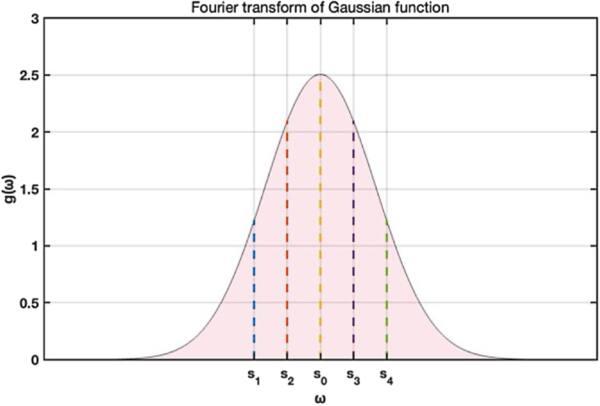
Figure 2. The Fourier spectra of a Gaussian function, where s0 = 0 and a phase factor $\exp ({\rm{i}}2\pi s\mu )$ as in equation ( |
With the Gaussian basis, we used five frequencies to approximate the profile of a Gaussian distribution in each reactant dimension. If there are d reactants, it seems that we need 5d points to mark a Gaussian profile, which indeed leads to the curse of dimensionality if d is large such as in a multi-species network. However, in fact, we do not have to use Gaussian basis in each dimension. They are only used in a few relevant dimensions and averages could be used in other dimensions by setting the formal variables to 1. In other words, we use certain marginal distribution to do the calculation and thus is able to avoid the dimensionality challenge. The relevant reactant dimensions include those involved in slow reactions and with small molecular copies or those having multi-stable states in the deterministic dynamics.
In the above, we extend the popular polynomial basis to the Fourier and the Gaussian basis, which provide a wide range of choices for the left observable functions. In face of a specific problem, we may choose an appropriate basis or even a combination of them according to the context. The deterministic results, the reaction topology and conservation laws are all important factors in this decision.
4. Numerical experiments
In this section, different choices of the left observable functions are applied to four typical examples of cell signaling pathways. In two examples—the Schlogl model and the genetic toggle switch, the deterministic equation gives two stable configurations. In the model of a second-order enzymatic reaction, a complex multimodal distribution emerges although deterministically only one stable state exists. The Heat shock response of Escherichia coli (E. coli) contains quite a few biochemical reactions and the distribution is a deformed Gaussion. Our computation works well and agrees nicely with the benchmark Gillespie (SSA) results but runs much faster.
4.1. The Schlogl model
The reactions of the Schlogl model are displayed in section 2.1 with pertinent parameter values in table 1 below. At the steady state, the probability density function of reactant X is bimodal. We compare the variational computations with different left observables, the moment basis equation (15 ) or a combination with the Fourier basis equation (16 ), where high-order derivatives are replaced by Fourier projections. This not only maintains the convenience of employing low-order moment basis but also avoids possible caveats caused by taking high-order derivatives.
Table 1. The parameter values for the schlogl model. |
| Figure | M | (c1, c2, c3, c4) |
|---|---|---|
| figure 3 | 3.0025 × 10⁵ | (3 × 10⁻⁷, 10−4, 10−3, 3.5) |
The probability distribution of molecule X at t = 1 is plotted in figure 3. The corresponding deterministic dynamics has two stable fixed points which leads to a bimodal distribution for the steady state in the random description. The benchmark is plotted as the gray shaded area while the pink dashed line depicts the result with equation (15 ), which grasped the bimodal profile but has considerable deviations in the position and the width. The solid line decorated with red circles used the Fourier basis, which almost overlaps with the benchmark produced by the stochastic simulation algorithm (SSA). Nevertheless, the variational method seems much more efficient in this example and the precise running time of the two programs is given in table 2 as a reference.
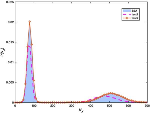
Figure 3. The probability distribution of NX at t = 1 in the Schlogl model from the Gillespie simulation (blue shaded area), the polynomial basis equation ( |
Table 2. Comparison of the running time of the Gillespie algorithm and the variational technique for the Schlogl model. |
| Time | Gillespie algorithm | Variational computation |
|---|---|---|
| t=1 | 4.159 × 10³ s | 10.317 s |
4.2. Genetic toggle switch
The gene switch is a very classical biological model, which is used to study the bistable behavior of gene expression. A simple version consists of two genes GeneA and GeneB, which leads to the production of two proteins A and B. Protein A and B can bind as dimers to each other’s gene promoter region to form bGeneB and bGeneA, inhibiting the respective gene expression. A cartoon genetic toggle switch model is portrayed in figure 4 which is developed by Schultz, Youfang [46–48] et al. The detailed reaction equations are given as follows:
$\begin{eqnarray}\begin{array}{l}{{\bf{R}}}_{{\bf{1}}}:\mathrm{GeneA}\mathop{\longrightarrow }\limits^{{c}_{1}}\mathrm{GeneA}+A,\\ {{\bf{R}}}_{{\bf{2}}}:\mathrm{GeneB}\mathop{\longrightarrow }\limits^{{c}_{2}}\mathrm{GeneB}+B,\\ {{\bf{R}}}_{{\bf{3}}}:{\rm{A}}\mathop{\longrightarrow }\limits^{{c}_{3}}{\rm{\varnothing }},\\ {{\bf{R}}}_{{\bf{4}}}:{\rm{B}}\mathop{\longrightarrow }\limits^{{c}_{4}}{\rm{\varnothing }},\\ {{\bf{R}}}_{{\bf{5}}}:2{\rm{A}}+\mathrm{GeneB}\mathop{\longrightarrow }\limits^{{c}_{5}}\mathrm{bGenB},\\ {{\bf{R}}}_{{\bf{6}}}:2{\rm{B}}+\mathrm{GeneA}\mathop{\longrightarrow }\limits^{{c}_{6}}\mathrm{bGeneA},\\ {{\bf{R}}}_{{\bf{7}}}:\mathrm{bGenB}\mathop{\longrightarrow }\limits^{{c}_{7}}2{\rm{A}}+\mathrm{GeneB},\\ {{\bf{R}}}_{{\bf{8}}}:\mathrm{bGeneA}\mathop{\longrightarrow }\limits^{{c}_{8}}2{\rm{B}}+\mathrm{GeneA},\end{array}\end{eqnarray}$
where c1, c2 are the protein synthesis rates, and c3, c4 the decay rates, while c5, c6 are the binding rates of the proteins with the genes, and c7, c8 denote the dissociation rates. Their values in the current computation are given in table 3.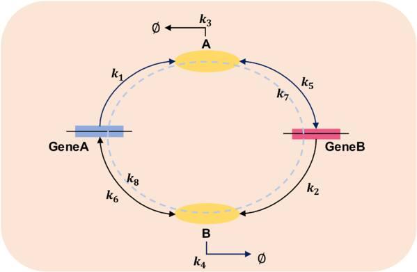
Figure 4. A genetic toggle switch model. |
Table 3. The parameter values for the genetic toggle switch. |
| Figure | (M1, M2, M3, M4) | (c1, c2, c3, c4, c5, c6, c7, c8) |
|---|---|---|
| figure 5 | (120, 80, 80, 80) | (40, 20, 1, 1, 1 × 10⁻⁵, 3.5 × 10⁻⁵, 1, 1) |
Deterministically, the genetic toggle switch network has two stable states since one protein’s presence inhibits the other’s production. Therefore, for the right basis we employ two distribution terms in a variable-separation form
$\begin{eqnarray}\begin{array}{l}{{\rm{\Psi }}}_{R}({x}_{1},{x}_{2},{x}_{3},{x}_{4},t)={f}_{17}{(1+{f}_{1}({x}_{1}-1))}^{{M}_{1}+{M}_{1}{f}_{2}}{x}_{1}^{-{M}_{1}{f}_{2}}\\ \,\times {(1+{f}_{3}({x}_{2}-1))}^{{M}_{2}+{M}_{2}{f}_{4}}{x}_{2}^{-{M}_{2}{f}_{4}}\\ \,\times {(1+{f}_{5}({x}_{3}-1))}^{{M}_{3}+{M}_{3}{f}_{6}}{x}_{3}^{-{M}_{3}{f}_{6}}\\ \,\times {(1+{f}_{7}({x}_{4}-1))}^{{M}_{4}+{M}_{4}{f}_{8}}{x}_{4}^{-{M}_{4}{f}_{8}}\\ \,+(1-{f}_{17}){(1+{f}_{9}({x}_{1}-1))}^{{M}_{1}+{M}_{1}{f}_{10}}{x}_{1}^{-{M}_{1}{f}_{10}}\\ \,\times {(1+{f}_{11}({x}_{2}-1))}^{{M}_{2}+{M}_{2}{f}_{12}}{x}_{2}^{-{M}_{2}{f}_{12}}\\ \,\times {(1+{f}_{13}({x}_{3}-1))}^{{M}_{3}+{M}_{3}{f}_{14}}{x}_{3}^{-{M}_{3}{f}_{14}}\\ \,\times {(1+{f}_{15}({x}_{4}-1))}^{{M}_{4}+{M}_{4}{f}_{16}}{x}_{4}^{-{M}_{4}{f}_{16}},\end{array}\end{eqnarray}$
where x1, x2, x3 and x4 are symbolic variables for molecules A, B, GeneA and GeneB. For the left observable function, we can use a combination of the polynomial basis and the Gaussian basis. The polynomial basis emphasizes the overall averages of molecular numbers, and the cross correlation between molecules, while the Gaussian observable checks the localized profiles in the state space. $\begin{eqnarray}\begin{array}{rcl}{{\rm{\Psi }}}_{L} & = & ({v}_{1}\partial {x}_{1}+{v}_{2}\partial {x}_{2}+{v}_{3}\partial {x}_{3}+{v}_{4}\partial {x}_{4}+{v}_{5}\partial {x}_{1}{x}_{3}\\ & & +\,{v}_{6}\partial {x}_{2}{x}_{3}+{v}_{7}\partial {x}_{2}{x}_{4}+{v}_{8}\partial {x}_{1}{x}_{4})\\ & & \times \left(\frac{\partial {{\rm{\Psi }}}_{R}}{\partial t}-{\rm{\Omega }}{{\rm{\Psi }}}_{R}\right){| }_{{x}_{1}={x}_{2}={x}_{3}={x}_{4}=1}\\ & & +\,{v}_{9}\displaystyle \sum _{j,n}{{\rm{\Pi }}}_{n}F({\theta }_{jn})\left(\frac{\partial {{\rm{\Psi }}}_{R}}{\partial t}-{\rm{\Omega }}{{\rm{\Psi }}}_{R}\right){| }_{\{{x}_{n}={{\rm{e}}}^{{\rm{i}}{\theta }_{jn}}\}}\\ & & +\,{v}_{10}\displaystyle \sum _{l,n}{{\rm{\Pi }}}_{n}F({\tilde{\theta }}_{ln})\left(\frac{\partial {{\rm{\Psi }}}_{R}}{\partial t}-{\rm{\Omega }}{{\rm{\Psi }}}_{R}\right){| }_{\{{x}_{n}={{\rm{e}}}^{{\rm{i}}{\tilde{\theta }}_{ln}}\}}.\end{array}\end{eqnarray}$
More specifically,(j = 0, 1, 2, 3, 4) and {θ0n = 0, θ1n = $\frac{{\mu }_{n}}{2\pi {\sigma }_{n}^{2}}-\frac{2}{{\sigma }_{n}}$, ${\theta }_{2n}=\frac{{\mu }_{n}}{2\pi {\sigma }_{n}^{2}}-\frac{1}{{\sigma }_{n}}$, ${\theta }_{3n}=\frac{{\mu }_{n}}{2\pi {\sigma }_{n}^{2}}+\frac{1}{{\sigma }_{n}}$, ${\theta }_{4n}=\frac{{\mu }_{n}}{2\pi {\sigma }_{n}^{2}}\,+\frac{2}{{\sigma }_{n}}{\}}_{(n=1,2)}$, where sets Gaussian profiles for molecule A and molecule B, so xothers = 1(θothers = 0) for other molecules, μn, σn are the position and the width of each reactant in the first term of equation (22 ). The variables $\{{\tilde{\theta }}_{ln}\}$ have similar expressions but are evaluated for the second term of equation (22 ). In the variable separation form equation (22 ), each factor has two parameters fa and fb defining
$\begin{eqnarray}\begin{array}{rcl}{\mu }_{\cdot } & = & {f}_{a}(M+M{f}_{b})-M{f}_{b},\\ {\sigma }_{\cdot } & = & (M+M{f}_{b})({f}_{a}-{f}_{a}^{2}).\end{array}\end{eqnarray}$
Note that in equation (23 ), we do not have 17 parameters as in equation (22 ) but a regularization condition may be used to give extra equations as explained in [37].
Below, we plot the probability distributions of reactants A and B in figures 5(a), (b) from the Gillespie algorithm (blue shaded areas) and the variational approach (red lines with circles). With the parameter in table 3, both A and B have a bimodal distribution and the results with different methods agree with each other very well. However, the variational approach has a much shorter running tine as is clearly shown in table 4.
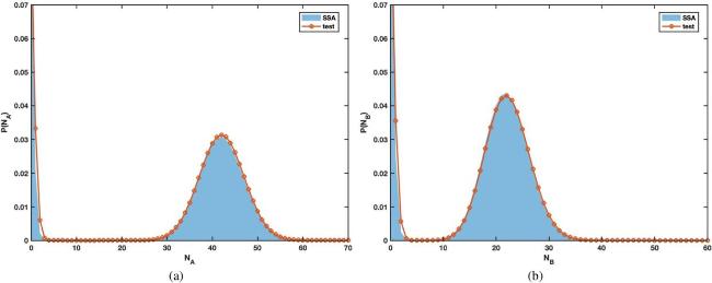
Figure 5. The probability distribution of NA(a) and NB(b) at t = 40 in the genetic Toggle switch model, computed with the Gillespie algorithm (blue shaded areas) or the variational technique (solid lines decorated with red circles). |
Table 4. Comparison of the running time of the Gillespie algorithm and the variational method for the genetic toggle switch model. |
| Time | Gillespie algorithm | Variation computation |
|---|---|---|
| t = 40 | 3.846 × 10⁴ s | 21.379 s |
4.3. Second-order enzymatic cascade
We consider a second-order enzymatic cascade that has applications in many biological processes, including metabolic pathways, signal transduction, and cell regulation [49–51]. With proper parameter values, multimodal distributions appear which constitute a good example to check our algorithm. The model contains the following chemical reactions
$\begin{eqnarray}\begin{array}{l}{{\bf{R}}}_{{\bf{1}}}:R\mathop{\longrightarrow }\limits^{{c}_{1}}{R}^{* },\\ {{\bf{R}}}_{{\bf{2}}}:{R}^{* }\mathop{\longrightarrow }\limits^{{c}_{2}}R,\\ {{\bf{R}}}_{{\bf{3}}}:A+{R}^{* }\mathop{\longrightarrow }\limits^{{c}_{3}}{A}^{* },\\ {{\bf{R}}}_{{\bf{4}}}:{A}^{* }\mathop{\longrightarrow }\limits^{{c}_{4}}A,\end{array}\end{eqnarray}$
where the receptor R is activated to R* at the rate of c1, and R* decays spontaneously to R at the rate of c2. The activated R* acts as an enzyme that catalyzes A to A* at rate c3 and A* decays spontaneously into A at rate c4. The values of the reaction rates in our computation are listed in table 5.From a physical point of view, if the first reaction is fast, the fluctuation in molecular number of R* is also fast, and we may use the average of R* to compute the dynamics of A*. If the first reaction is slow, the fluctuations of molecule R* will greatly affect the reaction A → A*, and the mean value of R* is not enough to characterize the dynamics, especially when this value is small. In that case, a Gaussian-like distribution of A* will be generated for each state of R*, which will be superimposed to make up the multi-modal distribution of A*, as depicted in figure 6.
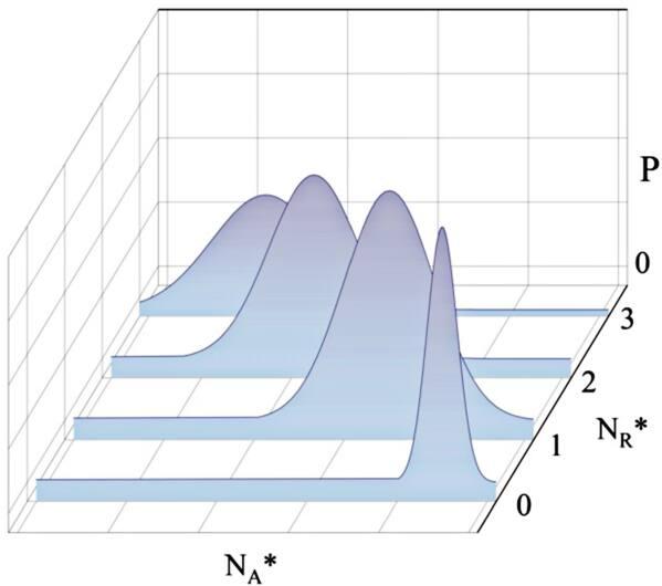
Figure 6. In case of extreme discreteness, the A* molecules reach a near-equilibrium distribution at each discrete state of R*. |
Considering the extreme discreteness of R* with the current parameter values, we use the following right test function [37]27 ), the first and second terms describe the mean number of molecules R* and A*, and the third and fourth terms for their variances. The fifth term depicts the correlation between molecule R* and A* while Gaussian basis captures multimodal distributions in the state space. Therefore, it combines the advantages of the overall statistical features and the individual peaks, accurately depicts the characteristics of the distribution, and at the same time maintains the convenience of the calculation.27 ) brings in the position and width information of the first term in equation (26 ), the third term for the second and the fourth term for the third, respectively. Still, a regularization condition is invoked to balance the number of equations and unknown variables ${\{{f}_{i}\}}_{i=1,\cdots \,,10}$ [37]. figures 7 and 8 respectively display the distribution profiles at different parameter values. In figure 7, when the discreteness of R* is not obvious, the probability distribution of A* is unimodal. In contrast, in figure 8, when the discreteness of R* is visible, a multi-modal distribution of A* is generated. The results compare well with the Gillespie simulation, whether it is unimodal or complex multi-modal. The running time of the two algorithms is shown in table 6.
$\begin{eqnarray}\begin{array}{l}{{\rm{\Psi }}}_{R}(x,t)={f}_{1}{(1+{f}_{5}({x}_{2}-1))}^{M}\\ \,+\,{f}_{2}{x}_{1}^{1}{(1+{f}_{6}({x}_{2}-1))}^{M}+{f}_{3}{x}_{1}^{2}{(1+{f}_{7}({x}_{2}-1))}^{M}\\ \,+\,{f}_{4}{x}_{1}^{3}{[{f}_{9}({x}_{1}{(1+{f}_{10}({x}_{2}-1))}^{M}-1)+1]}^{N}\\ \,\times \,{(1+{f}_{8}({x}_{2}-1))}^{M},\end{array}\end{eqnarray}$
where x1 and x2 mark R* and A*. In the left observable function, we used a combined form of polynomialand Gaussian basis. In the polynomial functions in equation ( $\begin{eqnarray}\begin{array}{rcl}{{\rm{\Psi }}}_{L} & = & ({v}_{1}\partial {x}_{1}+{v}_{2}\partial {x}_{2}+{v}_{3}\partial {x}_{1}{x}_{1}+{v}_{4}\partial {x}_{2}{x}_{2}+{v}_{5}\partial {x}_{1}{x}_{2})\\ & & \times \,\left(\frac{\partial {{\rm{\Psi }}}_{R}}{\partial t}-{\rm{\Omega }}{{\rm{\Psi }}}_{R}\right){| }_{{x}_{1}={x}_{2}=1}\\ & & +\,{v}_{6}\displaystyle \sum _{j,n}{{\rm{\Pi }}}_{n}F({\theta }_{jn})\left(\frac{\partial {{\rm{\Psi }}}_{R}}{\partial t}-{\rm{\Omega }}{{\rm{\Psi }}}_{R}\right){| }_{\{{x}_{n}={{\rm{e}}}^{{\rm{i}}{\theta }_{jn}}\}}\\ & & +\,{v}_{7}\displaystyle \sum _{l,n}{{\rm{\Pi }}}_{n}F({\tilde{\theta }}_{ln})\left(\frac{\partial {{\rm{\Psi }}}_{R}}{\partial t}-{\rm{\Omega }}{{\rm{\Psi }}}_{R}\right){| }_{\{{x}_{n}={{\rm{e}}}^{{\rm{i}}{\tilde{\theta }}_{ln}}\}}\\ & & +\,{v}_{8}\displaystyle \sum _{r,n}{{\rm{\Pi }}}_{n}F({\bar{\theta }}_{rn})\left(\frac{\partial {{\rm{\Psi }}}_{R}}{\partial t}-{\rm{\Omega }}{{\rm{\Psi }}}_{R}\right){| }_{\{{x}_{n}={{\rm{e}}}^{{\rm{i}}{\bar{\theta }}_{rn}}\}},\end{array}\end{eqnarray}$
where (j = 0, 1, 2, 3, 4) and (n = 1, 2), here the variables ${\theta }_{jn},{\tilde{\theta }}_{ln},{\bar{\theta }}_{rn}$ have similar expressions. The second term on the right of equation (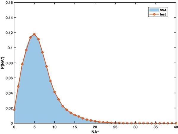
Figure 7. The probability distribution of ${N}_{{A}^{* }}$at t = 100, from the Gillespie algorithm (blue filled areas) or the variational approach (solid lines in red circles). The parameter values are displayed in table 5. |
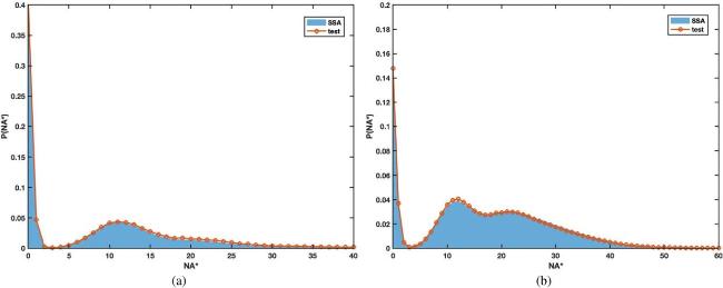
Figure 8. Probability distribution of ${N}_{{A}^{* }}$at t = 40(a) and t = 100(b) in the second-order enzyme cascade (equation ( |
Table 6. Comparison of the running time of the Gillespie algorithm and the variational approach in the second-order enzymatic cascade equation ( |
| Time | Gillespie algorithm | Variation computation |
|---|---|---|
| t = 40 | 7.958 × 10² s | 3.061 s |
| t = 100 | 9.412 × 10³ s | 3.834 s |
4.4. Heat shock response of E. coli
The heat shock response of Escherichia coli is a classic biological process [52–54]. When cells are stimulated by heating, a series of biochemical reactions are initiated to protect cells from high temperature damage, to repair damaged proteins, and to maintain cell homeostasis. One typical model [54] is sketched in figure 9 which includes the following 17 chemical reactions
$\begin{array}{l} \mathbf{R}_{\mathbf{1}}: \text { Protein } \xrightarrow{c_{1}} \text { UnfProt, } \\ \mathbf{R}_{\mathbf{2}}: \text { UnfProt }+ \text { DnaJ } \xrightarrow{c_{2}} \text { UnfProt_DnaJ, } \\ \mathbf{R}_{3}: \text { UnfProt_DnaJ } \xrightarrow{c_{3}} \text { Protein + DnaJ, } \\ \mathbf{R}_{\mathbf{4}}: \text { DNA_o32 } \xrightarrow{c_{4}} \text { mRNA_o32, } \\ \mathbf{R}_{\mathbf{5}}: \text { mRNA_o32 } \xrightarrow{c_{5}} \sigma 32, \\ \mathbf{R}_{\mathbf{6}}: \text { mRNA_o32 } \xrightarrow{c_{6}} \text { degrades, } \\ \mathbf{R}_{\mathbf{7}}: \sigma 32 \xrightarrow{c_{7}} \sigma 32_{\text {RNAP }}, \\ \mathbf{R}_{\mathbf{8}}: \sigma 32_{\text {RNAP }} \xrightarrow{c_{8}} \sigma 32, \\ \mathbf{R}_{\mathbf{9}}: \text { DNA_DnaJ }+\sigma 32_{\text {RNAP }}, \\ \quad \times \xrightarrow{c_{9}} \text { DNA_DnaJ }+\sigma 32+\text { DnaJ, } \\ \mathbf{R}_{\mathbf{1 0}}: \text { DNA_FtsH }+\sigma 32_{\text {RNAP, }} \\ \quad \times \xrightarrow{c_{10}} \text { DNA_FtsH }+\sigma 32+\text { FtsH, } \\ \mathbf{R}_{\mathbf{1 1}}: \text { DNA_GroEL }+\sigma 32_{\text {RNAP, }} \\ \quad \times \xrightarrow{c_{11}} \text { DNA_GroEL }+\sigma 32+\text { GroEL, } \\ \mathbf{R}_{\mathbf{1 2}}: \text { DnaJ } \xrightarrow{c_{12}} \text { degrades, } \\ \mathbf{R}_{\mathbf{1 3}}: \text { FtsH } \xrightarrow{c_{13}} \text { degrades, } \\ \mathbf{R}_{\mathbf{1 4}}: \text { GroEL } \xrightarrow{c_{14}} \text { degrades, } \\ \mathbf{R}_{\mathbf{1 5}}: \sigma 32+\text { DnaJ } \xrightarrow{c_{15}} \sigma 32 \text { DnaJ, } \\ \mathbf{R}_{\mathbf{1 6}}: \sigma 32 \text { DnaJ } \xrightarrow{c_{16}} \sigma 32+\text { DnaJ, } \\ \mathbf{R}_{\mathbf{1 7}}: \text { FtsH }+\sigma 32 \text { DnaJ } \xrightarrow{c_{17}} \text { DnaJ }+ \text { FtsH, } \end{array}$
where ${\{{c}_{i}\}}_{i=1,\cdots \,,17}$ are chemical reaction rates [54] with values given in table 7.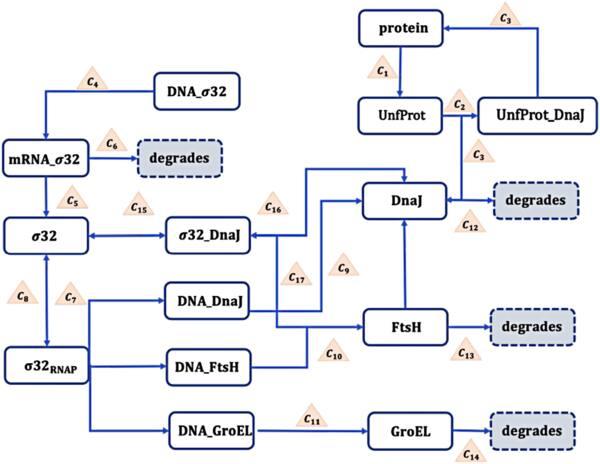
Figure 9. The heat shock response network of E. coli. |
Table 7. The parameter values for the heat shock response model of E. coli. |
| figure 10 |
|---|
| (M1, …, M11): (1 × 10⁷, 2 × 10⁶, 10, 50, 100, 20, |
| 10, 20, 700, 1 × 10³, 1 × 10⁴) |
| (c1, …, c17): (0.2, 0.0108, 0.2, 1.4 × 10⁻³, 0.07, 1.4 × 10⁻⁶, 0.7, 0.13, |
| 4.88 × 10⁻³, 4.88 × 10⁻³, 6.29 × 10⁻³, 6.4 × 10⁻¹⁰, 7.4 × 10⁻¹¹, |
| 1.8 × 10⁻⁸, 3.62 × 10⁻⁴, 4.4 × 10⁻⁴, 1.42 × 10⁻⁶) |
It is not hard to see from the above table that the reaction rates are very different, which indicates a large time scale separation and leads to low efficiency of general random simulation algorithms. Instead, if the variational technique is employed, only a finite set of ODEs need to be solved and many powerful algorithms could be utilized to speed up. Still, according to the deterministic dynamics, no extreme discreteness is present as in the previous example. Hence, we may use a variable-separation form as the right basis and assume
$\begin{eqnarray}\begin{array}{l}{{\rm{\Psi }}}_{R}(X,t)={(1+{f}_{1}({x}_{1}-1))}^{{M}_{1}+{M}_{1}{f}_{2}}{x}_{1}^{-{M}_{1}{f}_{2}}\\ \quad \times \,{(1+{f}_{3}({x}_{2}-1))}^{{M}_{2}+{M}_{2}{f}_{4}}{x}_{2}^{-{M}_{2}{f}_{4}}\\ \quad \times \,{(1+{f}_{5}({x}_{3}-1))}^{{M}_{3}+{M}_{3}{f}_{6}}{x}_{3}^{-{M}_{3}{f}_{6}}\\ \quad \times \,{(1+{f}_{7}({x}_{4}-1))}^{{M}_{4}+{M}_{4}{f}_{8}}{x}_{4}^{-{M}_{4}{f}_{8}}\\ \quad \times \,{(1+{f}_{9}({x}_{5}-1)+{f}_{10}({x}_{6}-1))}^{{M}_{5}+{M}_{5}{f}_{11}+{M}_{5}{f}_{12}}{x}_{5}^{-{M}_{5}{f}_{11}}{x}_{6}^{-{M}_{5}{f}_{12}}\\ \quad \times \,{(1+{f}_{13}({x}_{7}-1))}^{{M}_{6}+{M}_{6}{f}_{14}}{x}_{7}^{-{M}_{6}{f}_{14}}\\ \quad \times {(1+{f}_{15}({x}_{8}-1))}^{{M}_{7}+{M}_{7}{f}_{16}}{x}_{8}^{-{M}_{7}{f}_{16}}\\ \quad \times \,{(1+{f}_{17}({x}_{9}-1))}^{{M}_{8}+{M}_{8}{f}_{18}}{x}_{9}^{-{M}_{8}{f}_{18}}\\ \quad \times \,{(1+{f}_{19}({x}_{10}-1))}^{{M}_{9}+{M}_{9}{f}_{20}}{x}_{10}^{-{M}_{9}{f}_{20}}\\ \quad \times \,{(1+{f}_{21}({x}_{11}-1))}^{{M}_{10}+{M}_{10}{f}_{22}}{x}_{11}^{-{M}_{10}{f}_{22}}\\ \quad \times \,{(1+{f}_{23}({x}_{12}-1))}^{{M}_{11}+{M}_{11}{f}_{24}}{x}_{12}^{-{M}_{11}{f}_{24}},\end{array}\end{eqnarray}$
where $X={({x}_{1},...,{x}_{12})}^{t}$ marks different molecules: Protein, UnfProt, DNA_σ32, mRNA_σ32, σ32, σ32RNAP, DNA_DnaJ, DNA_FtsH, DNA_GroEL, DnaJ, FtsH, GroEL. Still, the left test function could be chosen as a combination of different strategies $\begin{eqnarray}\begin{array}{rcl}{{\rm{\Psi }}}_{L} & = & ({v}_{1}\partial {x}_{1}+{v}_{2}\partial {x}_{2}+{v}_{3}\partial {x}_{3}+{v}_{4}\partial {x}_{4}+{v}_{5}\partial {x}_{5}+{v}_{6}\partial {x}_{6}\\ & & +\,{v}_{7}\partial {x}_{7}+{v}_{8}\partial {x}_{8}+{v}_{9}\partial {x}_{9}+{v}_{10}\partial {x}_{10}\\ & & +\,{v}_{11}\partial {x}_{11}+{v}_{12}\partial {x}_{12})\\ & & \times \,\left(\frac{\partial {{\rm{\Psi }}}_{R}}{\partial t}-{\rm{\Omega }}{{\rm{\Psi }}}_{R}\right){| }_{({x}_{1},\ldots ,{x}_{12})=1}\\ & & +\,{v}_{13}\displaystyle \sum _{j,n}{{\rm{\Pi }}}_{n}F({\theta }_{jn})\left(\frac{\partial {{\rm{\Psi }}}_{R}}{\partial t}-{\rm{\Omega }}{{\rm{\Psi }}}_{R}\right)\\ & & \times \,{| }_{\{{x}_{5}={{\rm{e}}}^{{\rm{i}}{\theta }_{j5}},{x}_{10}={{\rm{e}}}^{{\rm{i}}{\theta }_{j10}},{x}_{others}=1\}}.\end{array}\end{eqnarray}$
The transcription factor σ32 is the main regulatory factor of Escherichia coli’s response to heat shock, which forms a complex with the heat shock protein DnaJ and is used to characterize important kinetic characteristics during the biochemical reaction process. Here the index ranges in the above equation are (j = 0, 1, 2, 3, 4) and (n = 5, 10). The last assignment in equation (30 ) put Gaussian profiles only for σ32(x5) and DnaJ(x10) and hence take xothers = 1(θothers = 0) for other molecules.
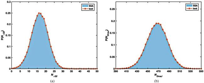
As plotted in figure 10, the probability distributions of two reactants σ32 (figure 10(a)) and DnaJ (figure 10(b)) agree very well with those by SSA. The profiles are quite close to but not exactly a Gaussian as the discreteness may still play a role due to the limited number of σ32. Regardless of the time scale separation, the variational approach seems to achieve a thousand times more efficiency than the Gillespie algorithm according to the running time shown in table 8, while the accuracy is maintained.
Figure 10. The probability distribution of Nσ32(a) and NDnaJ(b) at t = 100 in heat shock model of E. coli by the Gillespie algorithm (blue filled areas) and the variational technique (solid lines with red circles). |
Table 8. Comparison of the running time of the Gillespie algorithm and the variational approach in the heat shock response of E. coli. |
| Time | Gillespie algorithm | Variation computation |
|---|---|---|
| t = 100 | 1.720 × 10⁴ s | 11.061 s |
5. Conclusions
Signal transduction in biological cells is mostly a nonlinear noisy process with complex energy landscapes, which involves multiple molecular interactions and feedbacks. Hence, a wide span of time scales in reactions and copy numbers of different species are often seen, which makes popularly employed stochastic simulations slow or even inaccurate. In a previous paper [36], via a variational approach we found that the state of the stochastic dynamics actually has a low-dimensional structure in the distribution space, which could be captured by a properly selected trial generating function [37]. Nevertheless, with the increasing complexity of signal transduction networks, the conventional left observable functions required in the variational calculation become incompetent since the low-dimensional polynomial basis it provides is hard to capture highly localized profiles that frequently emerge in complex reaction chains.
To fill the caveat, in the current paper, two types of left observables are proposed: the Fourier basis and the Gaussian basis, which serve to capture multi-peaked distributions and the localized profiles without taking high-order derivatives in contrast to the conventional approach. By incorporating the position and width information of individual peaks, the characteristics of complex distributions are better captured, which significantly reduces the computational load and thus further confirms the low dimensionality of the distribution. The technique was applied to four typical reaction networks: the Schlogl model, the genetic toggle switch, a second-order enzymatic cascade and the heat shock model of E. coli and achieved nice accuracy and much improved efficiency, compared to the conventional Gillespie algorithm.
In the current paper, a projection through proper left and right test functions reveals the existence of analytic structures in the seemingly complex noisy signal transduction. Hence, a better understanding of the randomness is brought to the agenda and more efficient computational tools may be designed to interpret and predict disparate cellular responses. Nevertheless, how this analytic structure depends on the network structure, the parameter values, the numbers of molecules is not totally clear although some empirical statements have been made. Quantitative relations among these factors are well expected to remove the uncertainty in the design of the test functions and further reduce the computation load [37].