


1. Introduction
Coherent large vortex structures can occur in various bounded flows, with examples ranging from the Great Red Spot in Jupiter’s atmosphere [1], to giant vortex clusters in atomic Bose–Einstein condensates (BECs) [2, 3], and in dissipative quantum fluids of exciton–polaritons [4]. For a vortex system in a bounded domain, the phase space per vortex is also bounded. The formation of vortex clusters occurs because the system favors the clustering of like-sign vortices at high energies [5, 6]. Onsager formulated the statistical mechanics of a bounded point-vortex system in the microcanonical ensemble and demonstrated that the clustered state is at a negative absolute temperature. Since then, the clustering of vortices on bounded domains has been extensively investigated [7–36]. The clustering of vortices is also closely related to the end state of inverse energy cascades [29, 37, 38], which involves energy transport from small to large scales in two-dimensional (2D) turbulence.
Previous studies on Onsager vortices have mainly focused on systems confined on a flat region. Recent experimental realizations of BECs [39] and ultracold atomic bubbles [40] on the International Space Station have opened up the possibility of experimentally investigating bubble-trapped superfluids and vortex physics on curved surfaces. The curvature and topology of a surface have non-trivial effects on BECs [41–43], vortex dynamics [44–62], and the Berezinskii–Kosterlitz–Thouless (BKT) transition [63]. The formation and structure of Onsager vortices also strongly depend on the surface geometry. On a sphere, the distribution of a single species of vortices in the background of uniformly distributed vortices with opposite circulation has been studied in detail [23]. Recent numerical simulations of the point-vortex model, where low-energy vortex–antivortex pairs are removed, show that, unlike the giant dipole configuration of vortices confined to a disc [21, 24], uniformly distributed neutral vortices in a spherical shell trap form a quadruple cluster [31]. However, it is not clear whether the quadruple-clustered state is the most statistically favored state for a given energy, angular momentum, and vortex number. Answering this question requires studying the distributions of two species of vortices on a sphere simultaneously, which has not been thoroughly addressed.
In this paper, we systematically investigate the rotation-free clustered states of a neutral vortex system confined on a sphere. We extend the mean-field theory of vortex statistical mechanics developed by Joyce and Montgomery [7] to a sphere and treat the distributions of the two species of vortices simultaneously. In particular, we analyze the self-consistent equation of the stream function on a sphere near the uniform state and in the high energy limit. We find that, under the constraint of zero angular momentum, the sandwich state where vortices with opposite sign are distributed around the poles and the equator, respectively, is the maximum entropy state and it has higher statistical weight than the quadrupole state. For finite angular momentum, a giant dipole structure is statistically favored. The sandwich state and the dipole state are characterized by the non-vanishing quadrupole moment and the dipole moment, respectively. The energy dependence and the upper bounds of the quadrupole moment and the dipole moment at low energies and in the high-energy limit are also obtained within the mean-field theory. To test the mean-field predictions, we perform microcanonical Monte Carlo (MC) sampling with a number of finite vortices and find good agreement for the energy dependence of the quadrupole moment and the dipole moment for a system containing N = 1000 vortices. In addition, the values of the moments show saturation to the predicted upper bounds.
2. Point vortices on a sphere
For a superfluid on a plane, the circulation of a quantum vortex is quantized in units of circulation quantum κ ≡ 2πℏ/m [64], and the vorticity has a singularity at the vortex core ri: ω(r) = ∇ × u = κiδ(r − ri) = κσiδ(r − ri), with sign σi = ±1 for singly charged vortices. Here, m is the atomic mass and u is the superfluid velocity. The quantization ensures that the vorticity of a quantum vortex concentrates around the core region [6]. Hence, when the mean separation between quantum vortices $\bar{d}$ is much larger than the vortex core size ξ [65, 66], the point vortex model (PVM) describes the dynamics of quantum vortices in the incompressible limit effectively [5, 6, 67, 68], provided vortex annihilation can be neglected. In this limit, the flow is nearly incompressible ∇ · u = 0 and hence a stream function ψ can be introduced such that ${\boldsymbol{u}}={\rm{\nabla }}\psi \times \hat{{\boldsymbol{z}}}$, where $\hat{{\boldsymbol{z}}}$ is the unit vector normal to the plane. The stream function is completely determined by vortex positions and ψ(r) = −∑iκiG(r, ri), where $G({\boldsymbol{r}},{{\boldsymbol{r}}}_{i})\,=-(1/2\pi ){\mathrm{log}}\,(| {\boldsymbol{r}}-{{\boldsymbol{r}}}_{i}| /\xi )$ is the Green’s function of the Laplacian operator in 2D: ∇2G(r, ri) = −δ(r − ri). The PVM also describes 2D superfluid transition at finite temperature, which is the celebrated BKT transition [69, 70].
On curved surfaces, a covariant PVM has been well formulated [46, 48, 54]. Here we only focus on the PVM on a sphere. The Riemannian metric on a sphere is
$\begin{eqnarray}{\rm{d}}{s}^{2}={R}^{2}{\rm{d}}{\theta }^{2}+{R}^{2}{\sin }^{2}\theta {\rm{d}}{\phi }^{2},\end{eqnarray}$
where R is the radius, θ is the polar angle, and φ is the azimuthal angle.The Cartesian coordinates relate to the spherical coordinates via
$\begin{eqnarray}\xi =R\sin \theta \cos \phi ,\quad \eta =R\sin \theta \sin \phi ,\quad \zeta =R\cos \theta .\end{eqnarray}$
The projection from the north pole to the ζ = 0 plane induces stereographic coordinates z = x1 + ix2, where the x1 and x2 axes are identified as the ξ and η axes, respectively (figure 1). Let us also introduce the following notations ∂z ≡ (∂1 − i∂2)/2 and ${\partial }_{\bar{z}}\equiv ({\partial }_{1}+{\rm{i}}{\partial }_{2})/2$. In terms of stereographic coordinates, the metric reads ${\rm{d}}{s}^{2}=h({x}^{1},{x}^{2})[{({\rm{d}}{x}^{1})}^{2}+{({\rm{d}}{x}^{2})}^{2}]$, where $h=4{R}^{4}/{({R}^{2}+| z{| }^{2})}^{2}$. For a sphere, stereographic coordinates are isothermal coordinates [71] and are related to the spherical coordinates by $\begin{eqnarray}z=R\cot \left(\frac{\theta }{2}\right){{\rm{e}}}^{{\rm{i\phi }}}.\end{eqnarray}$
It is sometimes convenient to introduce polar coordinates z = ρeiφ, where $\rho =R\cot (\theta /2)$ and the polar angle φ is chosen to coincide with the azimuthal angle. The relations between the three coordinate systems are $\begin{eqnarray}\xi =\frac{2{x}^{1}{R}^{2}}{{R}^{2}+| z{| }^{2}}=\sqrt{h}{x}^{1}=R\sin \theta \cos \phi ,\end{eqnarray}$
$\begin{eqnarray}\eta =\frac{2{x}^{2}{R}^{2}}{{R}^{2}+| z{| }^{2}}=\sqrt{h}{x}^{2}=R\sin \theta \sin \phi ,\end{eqnarray}$
$\begin{eqnarray}\zeta =R\frac{{R}^{2}-| z{| }^{2}}{{R}^{2}+| z{| }^{2}}=R\cos \theta ,\,\end{eqnarray}$
and we use Cartesian, spherical or stereographic coordinates wherever convenient.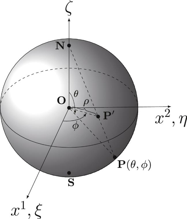
Figure 1. Stereographic projection from the north pole. The point P(θ, φ) on the southern hemisphere is projected onto the ζ = 0 plane and is denoted as ${{\rm{P}}}^{{\prime} }$. |
In spherical coordinates, the stream function reads
$\begin{eqnarray}\psi (\theta ,\phi )=\kappa \displaystyle \sum _{i}{\sigma }_{i}G(\theta ,\phi ;{\theta }_{i},{\phi }_{i}),\end{eqnarray}$
where (θi, φi) is the position of the ith vortex, G(θ, φ;θi, φi) is the Green’s function satisfying [48, 54] $\begin{eqnarray}{{\rm{\nabla }}}^{2}G(\theta ,\phi ;{\theta }_{i},{\phi }_{i})=-{\delta }_{s}(\theta ,\phi ;{\theta }_{i},{\phi }_{i})+1/{\rm{\Omega }},\end{eqnarray}$
where $\begin{eqnarray}{\delta }_{s}(\theta ,\phi ;{\theta }_{i},{\phi }_{i})=\frac{1}{{R}^{2}\sin \theta }\delta (\theta -{\theta }_{i})\delta (\phi -{\phi }_{i}),\end{eqnarray}$
Ω = 4πR2 is the area of the sphere, and ${{\rm{\nabla }}}^{2}\,=(1/\sin \theta ){\partial }_{\theta }(\sin \theta {\partial }_{\theta })+(1/{\sin }^{2}\theta ){\partial }_{\phi }^{2}$ is the Laplace–Beltrami operator. The Green’s function reads [48] $\begin{eqnarray}\begin{array}{rcl}G(\theta ,\phi ;{\theta }_{i},{\phi }_{i}) & = & -\frac{1}{2\pi }{\mathrm{log}}\,\frac{\sqrt{2{R}^{2}-2{\boldsymbol{r}}\cdot {{\boldsymbol{r}}}_{i}}}{\xi }\\ & = & -\frac{1}{2\pi }{\mathrm{log}}\,\left(\frac{\sqrt{2}R}{\xi }\sqrt{1-\cos {\rm{\Theta }}}\right),\end{array}\end{eqnarray}$
where Θ is the angle between r and ri, and $\cos {\rm{\Theta }}\,=\cos \theta \cos {\theta }_{i}+\sin \theta \sin {\theta }_{i}\cos (\phi -{\phi }_{i})$. It is interesting to notice that $\sqrt{2{R}^{2}-2{\boldsymbol{r}}\cdot {{\boldsymbol{r}}}_{i}}$ is the Euclidean distance, not the geodesic distance, between two points on the sphere.On a closed surface, the total vorticity must vanish, namely, ∑iσi = 0. Hence combining equations (7 ) and (8 ), we obtain
$\begin{eqnarray}{{\rm{\nabla }}}^{2}\psi (\theta ,\phi )=-\omega (\theta ,\phi ),\end{eqnarray}$
where $\begin{eqnarray}\omega (\theta ,\phi )=\kappa \displaystyle \sum _{i}{\sigma }_{i}\delta (\theta ,\phi ;{\theta }_{i},{\phi }_{i}).\end{eqnarray}$
The Hamiltonian of the point vortices on a sphere is $\begin{eqnarray}H=\frac{{\rho }_{s}{\kappa }^{2}}{2}\displaystyle \sum _{i\ne j}{\sigma }_{i}{\sigma }_{j}G({\theta }_{i},{\phi }_{i};{\theta }_{j},{\phi }_{j}).\end{eqnarray}$
On a sphere, besides the energy and the number of vortices, the quantities $\begin{eqnarray}{L}_{\xi }=\kappa {R}^{2}\displaystyle \sum _{i}{\sigma }_{i}\sin {\theta }_{i}\cos {\phi }_{i},\end{eqnarray}$
$\begin{eqnarray}{L}_{\eta }=\kappa {R}^{2}\displaystyle \sum _{i}{\sigma }_{i}\sin {\theta }_{i}\sin {\phi }_{i},\end{eqnarray}$
$\begin{eqnarray}{L}_{\zeta }=\kappa {R}^{2}\displaystyle \sum _{i}{\sigma }_{i}\cos {\theta }_{i},\,\end{eqnarray}$
are also conserved and are associated with the fluid angular momentum.3. Onsager vortex clusters on a sphere
3.1. Onsager vortex clusters at negative temperature
A particular feature of 2D point-vortex systems in a bounded domain is that the phase space area per vortex is finite. For a vortex system on a sphere, the phase space of a vortex is the spherical surface. Let us subdivide the surface into small cells of area ai ≪ Ω, where Ω is the surface area. While the cells are still large enough to contain many vortices. We consider a system consisting of N+ positive vortices and N− = N+ negative vortices. The total vortex number is N = N+ + N−. We denote the number of vortices in a cell of each species as ${N}_{i,\hat{\sigma }}$ with $\hat{\sigma }=\pm $ and the number of states is then given by [7, 72]
$\begin{eqnarray}{ \mathcal W }=\displaystyle \prod _{\hat{\sigma }}\left\{\displaystyle \prod _{i}\frac{{N}_{\hat{\sigma }}!}{{N}_{i,\hat{\sigma }}!}{\left(\frac{{a}_{i}}{{\rm{\Omega }}}\right)}^{{N}_{i,\hat{\sigma }}}\right\}.\end{eqnarray}$
The thermodynamic entropy is then ${k}_{B}{\mathrm{log}}\,{ \mathcal W }(H)$, where kB is the Boltzmann constant. Since ${k}_{{\rm{B}}}{\mathrm{log}}\,{ \mathcal W }(-\infty )\,={k}_{{\rm{B}}}{\mathrm{log}}\,{ \mathcal W }(+\infty )=0$, which corresponds to extreme situations of vortex–antivortex pairs collapsing and like-sign vortices concentrating into a point, respectively. Then ${ \mathcal W }$ must reach its maximum at an intermediate energy Hm and the inverse temperature $1/T\equiv {k}_{{\rm{B}}}\partial {\mathrm{log}}\,{ \mathcal W }(H)/\partial H$ is thus negative for H > Hm. High-energy states at negative temperature correspond to the formation of macroscopic vortex clusters [5, 6]. For given total vortex numbers N± and the area Ω, the entropy is a function of {Ni,±} and for large Ni,± we obtain $\begin{eqnarray}\begin{array}{rcl}(1/{N}_{\pm }){\mathrm{log}}\,{ \mathcal W } & \simeq & -\displaystyle \sum _{i}\left(\frac{{N}_{i,+}}{{N}_{+}{a}_{i}}{\mathrm{log}}\,\frac{{N}_{i,+}}{{N}_{+}{a}_{i}}\right){a}_{i}\\ & & -\displaystyle \sum _{i}\left(\frac{{N}_{i,-}}{{N}_{-}{a}_{i}}{\mathrm{log}}\,\frac{{N}_{i,-}}{{N}_{-}{a}_{i}}\right){a}_{i},\end{array}\end{eqnarray}$
where Stirling’s formula is applied and the irrelevant constants are ignored.3.2. Continuous limit and the mean-field theory
The PVM equation (13 ) exhibits Onsager clustered states at high energies. In clustered phases, the energy H ∼ N2; hence, in order to describe clustered phases in the proper thermodynamics limit, we need to make the rescaling σi → σi/N± and define the vortex number densities on a sphere as follows: 23 ) [plugging equations (7 ) and (12 ) into equation (23 )], we obtain that $E=H/{N}_{\pm }^{2}+{H}_{\,\rm{singular}\,}$, where ${H}_{\,\rm{singular}\,}\,=({\rho }_{s}{\kappa }^{2}/4\pi {N}_{\pm }^{2}){\sum }_{i}{\sigma }_{i}^{2}{\mathrm{log}}\,[d({{\boldsymbol{r}}}_{i},{{\boldsymbol{r}}}_{i})/\xi ]$, and d(ri, rj) is the Euclidean distance between the two points on a sphere. For point vortices, Hsingular = ∞. In practice, the distance between vortices can not be smaller than the vortex core size ξ which serves the ultraviolet cut-off of the PVM. By choosing d(ri, ri) = ξ, we have Hsingular = 0.
$\begin{eqnarray}{n}_{\pm }({\boldsymbol{r}})=\frac{1}{{N}_{\pm }}\displaystyle \sum _{i}^{{N}_{\pm }}{\delta }_{s}(\theta ,\phi ;{\theta }_{i},{\phi }_{i}),\end{eqnarray}$
where n± satisfies the normalization condition ∫dΩ n± = 1. The rescaled vortex charge density (vorticity) is then $\begin{eqnarray}\omega ({\boldsymbol{r}})=\kappa \sigma ({\boldsymbol{r}})\equiv \kappa [{n}_{+}({\boldsymbol{r}})-{n}_{-}({\boldsymbol{r}})],\end{eqnarray}$
and the rescaled stream function $\begin{eqnarray}\psi ({\boldsymbol{r}})=\kappa \int {\rm{d}}{{\rm{\Omega }}}^{{\prime} }G({\boldsymbol{r}},{{\boldsymbol{r}}}^{{\prime} })\,\sigma ({{\boldsymbol{r}}}^{{\prime} }),\end{eqnarray}$
satisfying $\begin{eqnarray}{{\rm{\nabla }}}^{2}\psi ({\boldsymbol{r}})=-\kappa \sigma ({\boldsymbol{r}}).\end{eqnarray}$
In the following, we consider vortex distributions at large scales and treat σ, n± and ψ as smooth functions at scales much larger than the mean separation $\bar{d}$. The rescaled coarse-grained Hamiltonian reads $\begin{eqnarray}\begin{array}{rcl}E & = & \frac{{\rho }_{s}{\kappa }^{2}}{2}\displaystyle \int {\rm{d}}{\rm{\Omega }}{\rm{d}}{{\rm{\Omega }}}^{{\prime} }\sigma ({\boldsymbol{r}})G({\boldsymbol{r}},{{\boldsymbol{r}}}^{{\prime} })\sigma ({{\boldsymbol{r}}}^{{\prime} })\\ & = & \frac{{\rho }_{s}}{2}\displaystyle \int {\rm{d}}{\rm{\Omega }}\,\omega ({\boldsymbol{r}})\psi ({\boldsymbol{r}}),\end{array}\end{eqnarray}$
and $E\sim { \mathcal O }(1)$. For a sphere, this Hamiltonian is just the rescaled kinetic energy of the flow generated by vortices: E = ρs/2∫dΩ ∣u∣2 = ρs/2∫dΩ ∣∇ψ∣2 = ρs/2∫dΩ ω ψ, where the fluid velocity u = ∇ψ × er and er is the radial unit vector. Applying point vortices directly to equation (In terms of the rescaled collective variables of vortices, the components of the angular momentum read
$\begin{eqnarray}{L}_{\xi }=\kappa {R}^{2}\int {\rm{d}}{\rm{\Omega }}\,\sigma \sin \theta \cos \phi ,\end{eqnarray}$
$\begin{eqnarray}{L}_{\eta }=\kappa {R}^{2}\int {\rm{d}}{\rm{\Omega }}\,\sigma \sin \theta \sin \phi ,\end{eqnarray}$
$\begin{eqnarray}{L}_{\zeta }=\kappa {R}^{2}\int {\rm{d}}{\rm{\Omega }}\,\sigma \cos \theta .\,\end{eqnarray}$
Hereafter, we choose the ζ-axis in the direction of total angular momentum, and hence L = Lζ, and we set ρs = κ = R = kB = 1 for convenience. In this convention $\xi \ll \bar{d}\ll 1$.In the continuous limit, ai → 0 and Ni,±/N±ai → n±(r), and the equation (18 ) gives rise to the thermodynamic entropy per vortex for given vortex distributions n± [6, 7]: 27 ) subject to given energy E, vortex number N±, and angular momentum Lζ:
$\begin{eqnarray}S[{n}_{+},{n}_{-}]=-\int {\rm{d}}{\rm{\Omega }}\left({n}_{+}{\mathrm{log}}\,{n}_{+}+{n}_{-}{\mathrm{log}}\,{n}_{-}\right),\end{eqnarray}$
and the most probable vortex density distribution is given by maximizing the entropy equation ( $\begin{eqnarray}\delta S-\beta \delta E-\alpha \delta {L}_{\zeta }-{\mu }_{+}\delta {N}_{+}/{N}_{+}-{\mu }_{-}\delta {N}_{-}/{N}_{-}=0,\end{eqnarray}$
where β and μ± are Lagrange multipliers and are determined by the energy and the number of vortices, having the interpretation of inverse temperature and chemical potentials in a microcanonical ensemble, respectively. Here, α is the Lagrange multiplier associated with the angular momentum and ω ≡ α/β has the meaning of rotation frequency.The variation equation (28 ) gives rise to 22 ) we obtain the self-consistent equation for determining the structure of coherent Onsager vortex clusters: 30 ) describe Onsager vortex states.
$\begin{eqnarray}{n}_{\pm }=\exp \left[\mp \beta \psi ({\boldsymbol{r}})\mp \alpha \cos \theta +{\gamma }_{\pm }\right],\end{eqnarray}$
where γ± = −μ± −1. Combining equation ( $\begin{eqnarray}\begin{array}{rcl}{{\rm{\nabla }}}^{2}\psi ({\boldsymbol{r}}) & = & \exp [\beta \psi ({\boldsymbol{r}})+\alpha \cos \theta +{\gamma }_{-}]\\ & & -\exp [-\beta \psi ({\boldsymbol{r}})-\alpha \cos \theta +{\gamma }_{+}].\end{array}\end{eqnarray}$
Non-uniform solutions at negative temperatures to equation (3.3. Onset of clustering
The onset of clustering involves global eigenmodes of the Laplace–Beltrami operator. It is then convenient to use spherical coordinates. Let us consider a solution to equation (30 ) for the given values of E and Lζ, and a nearby solution n± + δn± at E + δE and Lζ + δLζ. The corresponding changes in the constraints are 31 ), (32 ) and (33 ) then become 31 ) up to the leading order in δψ, we have 35 ) and (36 ), becomes
$\begin{eqnarray}0\,=\int {\rm{d}}{\rm{\Omega }}\,\delta {n}_{\pm },\,\end{eqnarray}$
$\begin{eqnarray}\delta E\,=\int {\rm{d}}{\rm{\Omega }}\psi \delta \sigma +\frac{1}{2}\int {\rm{d}}{\rm{\Omega }}\delta \sigma \delta \psi ,\end{eqnarray}$
$\begin{eqnarray}\delta {L}_{\zeta }\,=\int {\rm{d}}{\rm{\Omega }}\delta \sigma \cos \theta .\,\end{eqnarray}$
For the homogeneous state n± = n0 = 1/4π, and α = σ = ψ = 0. Equations ( $\begin{eqnarray}{{\rm{e}}}^{-\delta {\gamma }_{\pm }}={n}_{0}\int {\rm{d}}{\rm{\Omega }}\,\exp (\mp \beta \delta \psi +\delta \alpha \cos \theta ),\end{eqnarray}$
$\begin{eqnarray}\delta E=\frac{1}{2}\int {\rm{d}}{\rm{\Omega }}\,\delta \sigma \delta \psi ,\,\end{eqnarray}$
$\begin{eqnarray}\delta {L}_{\zeta }=\int {\rm{d}}{\rm{\Omega }}\delta \sigma \cos \theta .\,\end{eqnarray}$
Expanding δσ and equation ( $\begin{eqnarray}\delta \sigma =-2{n}_{0}(\beta \delta \psi -\delta {\gamma }_{+}+\cos \theta \delta \alpha ),\end{eqnarray}$
$\begin{eqnarray}\delta {\gamma }_{+}=-\delta {\gamma }_{-}=\beta {n}_{0}\int {\rm{d}}{\rm{\Omega }}\,\delta \psi ,\,\end{eqnarray}$
and, as it follows equations ( $\begin{eqnarray}\delta E=-{n}_{0}\int {\rm{d}}{\rm{\Omega }}\,(\beta \delta \psi -\delta {\gamma }_{+}+\cos \theta \delta \alpha )\delta \psi ,\end{eqnarray}$
$\begin{eqnarray}\delta {L}_{\zeta }=-2{n}_{0}\beta \int {\rm{d}}{\rm{\Omega }}\cos \theta \,\delta \psi -\frac{2}{3}\delta \alpha ,\,\end{eqnarray}$
where δα is assumed to be the same order as δψ.Combining equations (22 ) and (37 ), up to leading order in δψ, we obtain
$\begin{eqnarray}{{\rm{\nabla }}}^{2}\delta \psi =-\delta \sigma ({\boldsymbol{r}})=2{n}_{0}(\beta \delta \psi -\delta {\gamma }_{+}+\cos \theta \delta \alpha ).\end{eqnarray}$
Let us express the changes of the Lagrange multipliers in terms of the changes of the corresponding conserved quantities and introduce the operator ${ \mathcal P }$: 41 ) then becomes a zero-mode equation of the operator ${ \mathcal P }$, i.e.,
$\begin{eqnarray}\begin{array}{rcl}{ \mathcal P }\delta \psi & \equiv & {{\rm{\nabla }}}^{2}\delta \psi -2{n}_{0}\left[\beta \delta \psi -{n}_{0}\beta \displaystyle \int {\rm{d}}{\rm{\Omega }}\,\delta \psi \right.\\ & & \left.-3{n}_{0}\beta \cos \theta \displaystyle \int {\rm{d}}{\rm{\Omega }}\cos \theta \delta \psi -\frac{3}{2}\cos \theta \delta {L}_{\zeta }\right].\end{array}\end{eqnarray}$
Equation ( $\begin{eqnarray}{ \mathcal P }\delta \psi =0.\end{eqnarray}$
In order to solve the zero mode equation, we consider an expansion
$\begin{eqnarray}\delta \psi =\displaystyle \sum _{\ell =0}^{\infty }\displaystyle \sum _{m=-\ell }^{\ell }\epsilon {f}_{\ell m}{\psi }_{\ell m}(\theta ,\phi ),\end{eqnarray}$
where ψℓm satisfies ${ \mathcal P }{\psi }_{\ell m}=0$, fℓm is the mode coefficient, and ε ≪ 1 is a small amplitude. We denote δL = εL0, δα = εβω, and δE = ε2E0.We find that 43 ), if
$\begin{eqnarray}{\psi }_{\ell m}(\theta ,\phi )={c}_{\ell m}{\rm{Re}}({{\rm{Y}}}_{\ell m})+b\cos \theta \end{eqnarray}$
solves equation ( $\begin{eqnarray}\beta ={\beta }_{c,\ell }=-\frac{\ell (\ell +1)}{2{n}_{0}},\end{eqnarray}$
and b = −n0βω/(1 + n0β) for ℓ ≠ 1. While for ℓ = 1, b can be arbitrary and we choose that b = 0 without losing generality. Here Yℓm is the spherical harmonic function. For weakly clustered states, the vorticity field σ = σℓm ≡ δσ = εℓ(ℓ + 1)ψℓm.Given the values of E0 and L0, cℓm and ω are determined by
$\begin{eqnarray}{E}_{0}=-\frac{1}{2}\int {\rm{d}}{\rm{\Omega }}\,{\psi }_{\ell m}(\theta ,\phi ){{\rm{\nabla }}}^{2}{\,\psi }_{\ell m}(\theta ,\phi ),\end{eqnarray}$
$\begin{eqnarray}{L}_{0}=-2{n}_{0}{\beta }_{c,\ell }\int {\rm{d}}{\rm{\Omega }}\cos \theta {\psi }_{\ell m}-\frac{2}{3}{\beta }_{c,\ell }\omega .\,\end{eqnarray}$
For ℓ = m = 0, E0 = 0, and L0 = 0, hence only modes with ℓ > 0 are relevant. In the following, we focus on rotation-free states, namely ω = α = δα = 0, and in this case ${\psi }_{\ell m}={c}_{\ell m}{\rm{Re}}({{\rm{Y}}}_{\ell m})$.3.3.1. Dipole states: vortex-clustered states with finite angular momentum
Let us first consider the state with ℓ = 1 and m = 0, the corresponding stream function is
$\begin{eqnarray}{\psi }_{10}={c}_{10}{{\rm{Y}}}_{10}={c}_{10}\sqrt{\frac{3}{4\pi }}\cos \theta ,\end{eqnarray}$
where ${c}_{10}=\sqrt{{E}_{0}}$. This state carries finite angular momentum and L0 ≠ 0.The dipole moment is defined as
$\begin{eqnarray}{\boldsymbol{D}}\equiv \int {\rm{d}}{\rm{\Omega }}\,\sigma ({\boldsymbol{r}})\,{\boldsymbol{r}},\end{eqnarray}$
and for this state the dipole moment reads $\begin{eqnarray}{D}_{\eta }={D}_{\xi }=0\quad \,\rm{and}\,\quad {D}_{\zeta }=4\sqrt{\frac{\pi }{3}}\sqrt{E}.\end{eqnarray}$
We refer to this state as a dipole state and the onset of the dipole state occurs at $\beta ={\beta }_{c,1}\equiv {\beta }_{c}^{d}=-4\pi $. For the dipole state, the angular momentum ${L}_{\zeta }=4\sqrt{\pi /3}\sqrt{E}$. It is interesting to note that the vorticity distribution for the dipole state at low energies is identical to the vorticity distribution for a stationary vortex flow on a sphere [62] obtained via the vortex fluid theory.For m = ±1, the corresponding stream functions are ${\psi }_{11}=-{\psi }_{1,-1}={c}_{11}{\rm{Re}}({{\rm{Y}}}_{11})=-{c}_{11}\sqrt{3/8\pi }\sin \theta \cos \phi $, where ${c}_{11}\,=\sqrt{2}{c}_{10}$. These modes are connected by SO(3) rotation, namely, ψ11(r) = ψ10(r1) and r1 = R(0, π/2, 0) r. Here R(θ1, θ2, θ3) = Rζ(θ3)Rη(θ2)Rζ(θ1) is the SO(3) rotation operator and {θi=1,2,3} are the Euler angles. Therefore, modes ψ10, ψ11 and ψ1−1 describe the same dipole state but with different dipole moment orientations. Hereafter, we focus on the dipole state described by the mode ψ10 for which the dipole moment is along the ζ-axis [figure 2(a)].
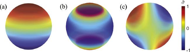
Figure 2. Rescaled vorticity $\tilde{\sigma }$ for the dipole (a), the sandwich (b) and the quadrupole (c) state. Here the extreme values of $\tilde{\sigma }$ are scaled to unity for convenience. |
3.3.2. Sandwich states: clusters with zero angular momentum
In this subsection, we consider clustered states with zero angular momentum L = 0 (or L0 = 0). Hence only modes with ℓ > 1 are relevant and δLζ = δα = 0. Intuitively, modes with larger ℓ describe a richer and finer structure and should have lower entropy. To ensure this is the case, let us expand S[n0 + δn−, n0 + δn+] around the uniform density n0 up to second order in δn±, and we obtain 31 ) and ${S}_{0}=-\int {\rm{d}}{\rm{\Omega }}\,2{n}_{0}{\mathrm{log}}\,{n}_{0}$ is the entropy for the homogeneous state. Here we have used $\delta {n}_{\pm }\,={n}_{0}[{{\rm{e}}}^{\delta {\gamma }_{\pm }}{{\rm{e}}}^{\mp \beta \delta \psi }-1]$ and equation (34 ) for δα = 0. To leading order in ε, δn± ≃ ∓ εn0βc,ℓψℓ,m and δγ± = 0, then equation (52 ) becomes A ).
$\begin{eqnarray}\begin{array}{rcl}S & = & {S}_{0}-\frac{1}{2{n}_{0}}\displaystyle \int {\rm{d}}{\rm{\Omega }}\left[{(\delta {n}_{+})}^{2}+{(\delta {n}_{-})}^{2}\right]+{ \mathcal O }(\delta {n}_{\pm })\\ & = & {S}_{0}-\frac{1}{2{n}_{0}}\left[{\left(\displaystyle \int {\rm{d}}{\rm{\Omega }}\,{{\rm{e}}}^{-\beta \delta \psi }\right)}^{-2}\displaystyle \int {\rm{d}}{\rm{\Omega }}\,{{\rm{e}}}^{-2\beta \delta \psi }\right.\\ & & +\left.{\left(\displaystyle \int {\rm{d}}{\rm{\Omega }}\,{{\rm{e}}}^{\beta \delta \psi }\right)}^{-2}\displaystyle \int {\rm{d}}{\rm{\Omega }}\,{{\rm{e}}}^{2\beta \delta \psi }-2{n}_{0}\right]+{ \mathcal O }(\delta {n}_{\pm }),\end{array}\end{eqnarray}$
where the first-order term in δn± vanishes due to the constraint equation ( $\begin{eqnarray}\begin{array}{rcl}S & \simeq & {S}_{0}-\left[{n}_{0}{\beta }_{c,\ell }^{2}\displaystyle \int {\rm{d}}{\rm{\Omega }}\,{\psi }_{\ell m}^{2}\right]{\epsilon }^{2}\\ & = & {S}_{0}-\frac{1}{{E}_{0}}\left[{n}_{0}{\beta }_{c,\ell }^{2}\displaystyle \int {\rm{d}}{\rm{\Omega }}\,{\psi }_{\ell m}^{2}\right]\delta E,\end{array}\end{eqnarray}$
and one can easily show that modes with ℓ = 2 have higher statistical weight (larger entropy) than the modes with ℓ > 2 (see Appendix Hence we only need to focus on states with ℓ = 2. For m = 0,
$\begin{eqnarray}{\psi }_{20}={c}_{20}{{\rm{Y}}}_{20}=\frac{{c}_{20}}{4}\sqrt{\frac{5}{\pi }}(3{\cos }^{2}\theta -1),\end{eqnarray}$
where ${c}_{20}=\sqrt{{E}_{0}/3}$. This mode describes the clustering of positive (negative) vortices around the poles and negative (positive) vortices around the equator [figure 2(b)]. We refer to this state as a sandwich state. The onset of the sandwich state occurs at β = βc,2 ≡ βc = −12π. For m = 1 and m = 2, ${\psi }_{22}(\theta ,\phi )={c}_{22}{\rm{Re}}({{\rm{Y}}}_{22})=({c}_{22}/4)\sqrt{15/2\pi }\cos (2\phi ){\sin }^{2}\theta $, ${\psi }_{21}(\theta ,\phi )\,={c}_{21}{\rm{Re}}({{\rm{Y}}}_{21})=-({c}_{21}/4)\sqrt{15/2\pi }\cos \phi \sin 2\theta $, where ${c}_{22}\,={c}_{21}=\sqrt{2{E}_{0}/3}$. Here, the two modes are also connected by SO(3) rotation, i.e., ψ21(r2) = ψ22(r), where r2 = R(− π/4, π/2, π/2) r. Therefore, modes ψ22 and ψ21 describe the same state and we refer to this state as a quadrupole state. Note that ψ2,−2 = ψ2,2 and ψ2,−1 = −ψ2,1. Hereafter, we focus on the quadrupole state described by the mode ψ21 [figure 2(c)].For states with ℓ = 2, the dipole moment D vanishes. In order to quantify the clustered states with zero angular momentum, it is necessary to introduce the quadrupole tensor
$\begin{eqnarray}{{ \mathcal Q }}_{ij}\left[\sigma ({\boldsymbol{r}})\right]\equiv \displaystyle \frac{1}{2}\int {\rm{d}}{\rm{\Omega }}\,\left[3({\boldsymbol{r}}\cdot {{\boldsymbol{e}}}_{{i}})({\boldsymbol{r}}\cdot {{\boldsymbol{e}}}_{{j}})-{\delta }_{ij}\right]\sigma ({\boldsymbol{r}}),\end{eqnarray}$
where {ei=ξ,η,ζ} are unit vectors in Cartesian coordinates. The quadrupole moment is defined as $\begin{eqnarray}Q[\sigma ]\equiv \sqrt{{q}_{1}^{2}+{q}_{2}^{2}+{q}_{3}^{2}},\end{eqnarray}$
where {q1, q2, q3} are eigenvalues of ${{ \mathcal Q }}_{ij}$. We denote Qs and Qq as the quadrupole moments for the sandwich and quadrupole states, respectively.For the sandwich state,
$\begin{eqnarray}{ \mathcal Q }[{\sigma }_{20}]=\epsilon {c}_{20}\sqrt{\frac{36\pi }{5}}\left(\begin{array}{ccc}-1 & 0 & 0\\ 0 & -1 & 0\\ 0 & 0 & 2\\ \end{array}\right),\end{eqnarray}$
and its eigenvalues are $\epsilon {c}_{20}\sqrt{36\pi /5}\,\{-1,-1,2\}$. The corresponding quadrupole momentum is $\begin{eqnarray}{Q}_{s}=Q[{\sigma }_{20}]={Q}_{0}| E-{E}_{c}{| }^{\nu },\end{eqnarray}$
where ν = 1/2, ${Q}_{0}=\sqrt{216\pi /15}$, and Ec = 0. For the quadrupole state, $\begin{eqnarray}{ \mathcal Q }[{\sigma }_{21}]=-\epsilon {c}_{21}\sqrt{\frac{54\pi }{5}}\left(\begin{array}{ccc}0 & 0 & 1\\ 0 & 0 & 0\\ 1 & 0 & 0\\ \end{array}\right),\,\end{eqnarray}$
and the eigenvalues of ${ \mathcal Q }[{\sigma }_{21}]$ are $-{c}_{21}\epsilon \sqrt{54\pi /5}\,\{-1,0,1\}$. The corresponding quadrupole momentum takes the same value as for the sandwich state, namely, Qq = Qs. Note that since σ21(Rr) = σ22(r), it is easy to see that ${ \mathcal Q }[{\sigma }_{21}]\,=R{ \mathcal Q }[{\sigma }_{22}]{R}^{T}$, where R = R( − π/4, π/2, π/2).Applying equation (53 ), we find that up to order δE, the sandwich state and the quadrupole state have the same entropy and the entropy difference appears in order δE2:
$\begin{eqnarray}S[{\rm{sandwich}}]-S[{\rm{quadrupole}}]\simeq \frac{5{\beta }_{c}^{4}{E}_{0}^{2}{\epsilon }^{4}}{576{\pi }^{2}}=\frac{5{\beta }_{c}^{4}}{576{\pi }^{2}}{(\delta E)}^{2}.\end{eqnarray}$
Hence, under the condition of zero angular momentum, the sandwich state has the highest statistical weight. Although this conclusion is drawn based on perturbative analysis at low energies, it will be confirmed by later analysis at high energies and Monte Carlo simulations at moderate energies. Here it is interesting to note that, unlike the other states (dipole and quadrupole states), when exchanging the circulation σi → −σi, the two corresponding sandwich states cannot be connected by SO(3) rotation and hence should be regarded as two distinct states.3.4. High-energy configurations
In this subsection, we consider the sandwich state and the dipole state at high energies. In the high energy limit, vortices and antivortices are well separated and are concentrated in small regions of a sphere. It is then convenient to use the stereographic projection method to find approximate density distributions of the vortices on a sphere.
In stereographic coordinates, equation (30 ) becomes
$\begin{eqnarray}(1+z{\bar{z})}^{2}{\partial }_{z}{\partial }_{\overline{z}}\psi ={{\rm{e}}}^{\beta \psi (z,\bar{z})+{\gamma }_{-}}-{{\rm{e}}}^{-\beta \psi (z,\bar{z})+{\gamma }_{+}},\end{eqnarray}$
for rotation-free states (ω = α = 0). The stereographic projection maps the southern hemisphere onto a disc on the ζ = 0 plane (figure 1) and transforms vortices in the region around southern pole and vortices in the region around the equator to the region around the origin and the region near the boundary of the disc, respectively.3.4.1. Sandwich states at high energies
In the high-energy limit, the interaction between vortices near the poles and antivortices near the equator can be neglected. For ∣z∣ ≪ 1, equation (61 ) is well approximated as
$\begin{eqnarray}{\partial }_{z}{\partial }_{\overline{z}}\psi =-{{\rm{e}}}^{-\beta \psi (z,\bar{z})+{\gamma }_{+}},\end{eqnarray}$
which can be regarded as the mean-field equation for describing distributions of chiral vortices confined to a (flat) disc and is well-defined on the whole disc domain. Hence finding the approximate distribution of vortices near the poles at high energies boils down to searching for distributions of chiral vortices confined to a disc with proper boundary conditions.For axisymmetric distributions, equation (62 ) becomes 54 ) at low energies. In addition, the vortex density distribution equation (65 ) does not depend on the value of ψ(ρ = 0) and here we choose ψ(ρ = 0) = 0 for convenience (see Appendix B ). We emphasize again that the exact solution to equation (64 ) is valid for the whole disc, while providing a good approximation of the distribution of vortices near the poles at large energies.
$\begin{eqnarray}\frac{1}{4}\frac{1}{\rho }\frac{{\rm{d}}}{{\rm{d}}\rho }\left(\rho \frac{{\rm{d}}}{{\rm{d}}\rho }\psi \right)=-{{\rm{e}}}^{-\beta \psi (\rho )+{\gamma }_{+}},\end{eqnarray}$
and has the following exact solution $\begin{eqnarray}\psi (\rho )=-\displaystyle \frac{2}{\beta }{\mathrm{log}}\,\left(\displaystyle \frac{2}{\beta {\rho }^{2}{{\rm{e}}}^{{\gamma }_{+}}-2}\right),\end{eqnarray}$
with boundary condition $\psi (\rho =0)={\psi }^{{\prime} }(\rho ){| }_{\rho =0}=0$ [13, 14, 32, 36]. Here, the boundary condition ${\psi }^{{\prime} }(\rho ){| }_{\rho =0}=0$ for the problem of chiral vortices confined to a disc is induced by the flow generated by the vortices on the sphere and can be obtained from the global stream function equation (The vortex density then reads
$\begin{eqnarray}{n}_{+}(\rho )=\exp (-\beta \psi +{\gamma }_{+})=\frac{4{{\rm{e}}}^{{\gamma }_{+}}}{{(\beta {\rho }^{2}{{\rm{e}}}^{{\gamma }_{+}}-2)}^{2}}.\end{eqnarray}$
For the sandwich state, since only half of the positive vortices are distributed around the south pole (the other half are distributed around the north pole), the normalization condition is $\begin{eqnarray}\frac{1}{2}={\int }_{0}^{2\pi }{\rm{d}}\phi {\int }_{0}^{1}\frac{4\rho }{{(1+{\rho }^{2})}^{2}}\,{\rm{d}}\rho \,{n}_{+}(\rho ),\end{eqnarray}$
which gives rise to the relation between ${{\rm{e}}}^{{\gamma }_{+}}$ and β [figure C.1(a) in the Appendix].When β → βs = −16π, vortices around the pole collapse into a point, known as supercondensation. Hence, the parameter range for the sandwich state is βs < β < βc. The limit configuration at β = βs is ${n}_{+}(\theta )\,=[\delta (\theta )\,+\delta (\theta \,-\pi )]/(4\pi \sin \theta )$. It is worthwhile mentioning that the value of βs depends on the normalization condition. For vortices confined to a disc on a plane, the vortex density profile is the same as equation (65 ); however, the vortex number is normalized to unity, which gives rise to βs = −8π (in the convention of this paper) [13, 14, 24, 32, 36].
In spherical coordinates, the stream function and the vortice density on the southern hemispheres [θ ∈ (π/2, π)] are [see also figure 3(a)]
$\begin{eqnarray}\psi (\theta )=-\frac{2}{\beta }{\mathrm{log}}\,\left[\frac{2}{\beta {\cot }^{2}\left(\frac{\theta }{2}\right){{\rm{e}}}^{{\gamma }_{+}}-2}\right],\end{eqnarray}$
$\begin{eqnarray}{n}_{+}(\theta )=\frac{4{{\rm{e}}}^{{\gamma }_{+}}}{{\left[\beta {\cot }^{2}\left(\frac{\theta }{2}\right){{\rm{e}}}^{{\gamma }_{+}}-2\right]}^{2}}.\,\end{eqnarray}$
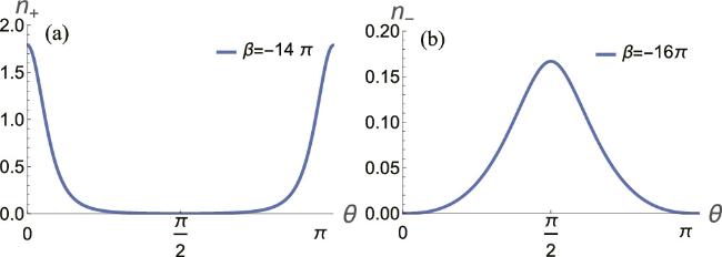
Figure 3. The vortex density distributions for the sandwich state at high energies. (a) The distribution of positive vortices near poles [equation ( |
Now we consider the distribution of negative vortices in the region near the equator, which is mapped to the region near the edge of the disc. For ∣z∣ ∼ 1, equation (61 ) is well approximated as 69 ) becomes 71 ) to the problem of chiral vortex clusters in a disc with the boundary condition equation (72 ) is well-defined on the whole disc domain and provides a good approximation of the distribution of vortices near the equator at large energies.
$\begin{eqnarray}4{\partial }_{z}{\partial }_{\overline{z}}\psi ={{\rm{e}}}^{\beta \psi (z,\bar{z})+{\gamma }_{-}}.\end{eqnarray}$
For axis-symmetric solutions, equation ( $\begin{eqnarray}\frac{1}{\rho }\frac{{\rm{d}}}{{\rm{d}}\rho }\left(\rho \frac{{\rm{d}}}{{\rm{d}}\rho }\psi \right)={{\rm{e}}}^{\beta \psi (\rho )+{\gamma }_{-}},\end{eqnarray}$
which admits an exact solution $\begin{eqnarray}\psi (\rho )=\frac{2}{\beta }{\mathrm{log}}\,\left(\frac{2A{\rho }^{(-1+A/2)}}{2+A+(A-2){\rho }^{A}}\right),\end{eqnarray}$
with the boundary condition [36] $\begin{eqnarray}\psi (\rho =1)={\psi }^{{\prime} }(\rho ){| }_{\rho =1}=0,\end{eqnarray}$
and $A=\pm \sqrt{4-2\beta {{\rm{e}}}^{{\gamma }_{-}}}$. Similarly, the exact solution equation (It follows that the density is 54 ). The vortex density distribution equation (73 ) is independent of the value of ψ(ρ = 1) and here we choose ψ(ρ = 1) = 0 for convenience (see Appendix B ). The relation between ${{\rm{e}}}^{{\gamma }_{-}}$ and β is given by the normalization condition equation (66 ) (n+ → n−). Moreover, the smooth condition ${n}_{-}^{{\prime} }(\rho ){| }_{\rho =0}=0$ requires ${{\rm{e}}}^{{\gamma }_{-}}\beta \lt -5/2$, which gives rise to β < −7.11π [figure C.1(b) in the Appendix]. Hence, for β within the range βs < β < βc, the smooth condition is automatically satisfied.
$\begin{eqnarray}{n}_{-}(\rho )=\frac{4{A}^{2}{\rho }^{(A-2)}{{\rm{e}}}^{{\gamma }_{-}}}{{\left[2+A+(A-2){\rho }^{A}\right]}^{2}}.\end{eqnarray}$
Note that the boundary condition ${\psi }^{{\prime} }(\rho ){| }_{\rho =1}=0$ is also induced by the global stream function equation (In spherical coordinates, the stream function and the vortex density distribution of negative vortices near the equator [θ ∈ (π/2, π)] read 72 ), the fluid velocity uφ = −∂ψ(θ)/∂θ on the equator vanishes, namely uφ(θ = π/2) = 0, which is consistent with the fluid velocity field on the equator at low energies [${\psi }_{20}^{{\prime} }(\theta ){| }_{\theta =\pi /2}=0$]. At β = βs, ${{\rm{e}}}^{{\gamma }_{-}}\approx 0.167,A\approx 4.556$ [figure C.1(b) in the Appendix], the vorticity for the sandwich state reads ${\sigma }_{s}({\boldsymbol{r}})\,=\left[\delta (\theta )+\delta (\theta -\pi )\right]/(4\pi \sin \theta )-{n}_{-}(\theta ),$ and the quadrupole moment reaches the maximum value ${Q}_{s}^{{\rm{\max }}}\,\approx 1.59$. It is easy to see that the quadrupole state also reaches the high-energy limit at β = βs, and the corresponding vorticity is ${\sigma }_{q}({\boldsymbol{r}})=\delta (\theta -\pi /4,\phi )+\delta (\theta -3\pi /4,\phi -\pi )-\delta (\theta \,-3\pi /4,\phi )-\delta (\theta -\pi /4,\phi -\pi )/(2\sin \theta )$, which gives rise to the maximum quadrupole moment ${Q}_{q}^{{\rm{\max }}}=3\sqrt{2}/2\gt {Q}_{s}^{{\rm{\max }}}$. Note that the quadrupole state locations of the clusters at supercondensation coincide with mechanical equilibrium positions for four-point vortices on a sphere.
$\begin{eqnarray}\psi (\theta )=\frac{2}{\beta }{\mathrm{log}}\,\left[\frac{2A\cot {(\theta /2)}^{(-1+A/2)}}{2+A+(A-2)\cot {(\theta /2)}^{A}}\right],\end{eqnarray}$
$\begin{eqnarray}{\,n}_{-}(\theta )=\frac{4{A}^{2}{\cot }^{(A-2)}(\theta /2){{\rm{e}}}^{{\gamma }_{-}}}{{\left[2+A+(A-2){\cot }^{A}(\theta /2)\right]}^{2}}.\,\end{eqnarray}$
Induced by the boundary condition equation (3.4.2. General solutions
A general solution to equation (62 ) is available [73, 74]:
$\begin{eqnarray}\psi (z,\overline{z})=-\frac{1}{\beta }{\mathrm{log}}\,\left[\frac{2{f}^{{\prime} }(z)\overline{{f}^{{\prime} }(z)}}{-c\beta {(1+f(z)\overline{f(z)})}^{2}}\right],\end{eqnarray}$
$\begin{eqnarray}n(z,\overline{z})=c\exp (-\beta \psi ),\,\end{eqnarray}$
where f(z) is a meromorphic function of z in a simply connected domain and $\overline{f(z)}$ is the complex conjugate of f(z). Furthermore, it is required that f(z) has at most simple poles and ${f}^{{\prime} }(z)\ne 0$ in the consider domain [45, 74].Here, we show that equations (64 ) and (71 ) fall into this general solution by specifying function f(z) properly. For an axisymmetric distribution, the stream function $\psi (z,\overline{z})$ must be the function of $z\overline{z}$ or ρ only. Hence f(z) has a unique form and f(z) = azb, here $a\in {\mathbb{C}},b\in {\mathbb{Z}}$. The boundary condition $\psi (\rho =0)={\psi }^{{\prime} }(\rho ){| }_{\rho =0}=0$ determines that $a=\sqrt{-c\beta /2}$, b = 1, and $c={{\rm{e}}}^{{\gamma }_{+}}$, which leads to equation (64 ) precisely. The general solution to equation (76 ) gives rise to equation (71 ) by choosing $f(z)=\,\sqrt{(A-2)/(A+2)}\,{z}^{A/2}$, where $A=\pm \sqrt{4-2\beta {{\rm{e}}}^{{\gamma }_{-}}}$, and $c={{\rm{e}}}^{{\gamma }_{-}}/4$. Here, the boundary condition $\psi (\rho =1)={\psi }^{{\prime} }(\rho ){| }_{\rho =1}=0$ is fulfilled. An observation can be made here: the exponent A/2 is not an integer in general. Hence such a choice of f(z) may not be a meromorphic function and then does not meet the requirements for equation (76 ). As shown previously, such a solution is indeed the solution to equation (70 ), suggesting that the validity condition of equation (77 ) may be extended.
3.4.3. Dipole states at high energies
At high energies, for the dipole state, vortices with opposite sign are concentrated near the poles. The density distribution of positive vortices near the southern pole is identical to equation (65 ) and the only difference is that here the vortex density is normalized to unity but not 1/2. Hence, for the dipole state, the supercondensation occurs at $\beta ={\beta }_{s}^{d}=-8\pi $, which is the same as that for vortices confined to a disc on a plane [13, 24, 36].
In spherical coordinates, the vortex densities are (see also figure 4)
$\begin{eqnarray}{n}_{-}(\theta )=\frac{4{{\rm{e}}}^{{\gamma }_{-}}}{{\left[\beta {\cot }^{2}(\theta /2){{\rm{e}}}^{{\gamma }_{-}}-2\right]}^{2}}\quad \theta \in (\pi /2,\pi ),\end{eqnarray}$
$\begin{eqnarray}{n}_{+}(\theta )=\frac{4{{\rm{e}}}^{{\gamma }_{+}}}{{\left[\beta {\tan }^{2}(\theta /2){{\rm{e}}}^{{\gamma }_{+}}-2\right]}^{2}}\quad \theta \in (0,\pi /2),\end{eqnarray}$
and the corresponding angular momentum is $\begin{eqnarray}\begin{array}{rcl}{L}_{\zeta }(\beta ) & = & \frac{8\pi {{\rm{e}}}^{{\gamma }_{-}}}{{(2+\beta {{\rm{e}}}^{{\gamma }_{-}})}^{4}}\left[\beta {{\rm{e}}}^{{\gamma }_{-}}\left(\beta {{\rm{e}}}^{{\gamma }_{-}}(-2\beta +5+32{\mathrm{log}}\,2)\right.\right.\\ & & \left.+20-32{\mathrm{log}}\,2\right)-16\beta {{\rm{e}}}^{{\gamma }_{-}}(\beta {{\rm{e}}}^{{\gamma }_{-}}-1)\\ & & \left.\times \,{\mathrm{log}}\,(2-\beta {{\rm{e}}}^{{\gamma }_{-}})+4\right].\end{array}\end{eqnarray}$
When $\beta \to {\beta }_{s}^{d}$, ${n}_{-}\to \,\delta (\theta \,-\,\pi )/(2\pi \sin \theta ),{n}_{+}\to \,\delta (\theta )/(2\pi \sin \theta )$, and the angular momentum reaches the upper bound ${L}_{\zeta }\,\to {L}_{\zeta }^{{\rm{\max }}}=2$.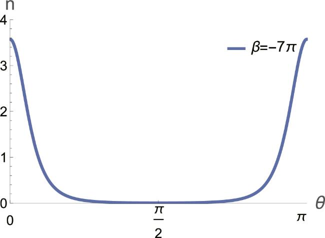
Figure 4. The total vortex density for the dipole state at high energies [equations ( |
We now consider the flow generated by these vortices. The fluid velocity field reads u = ∇ψ × er = uθeθ + uφeφ, where er, eθ, eφ are three orthogonal spherical unit vectors. For the dipole state at low energies, ${u}_{\theta }=(1/\sin \theta )\partial \psi /\partial \phi =0$, ${u}_{\phi }\,=-\partial \psi /\partial \theta \propto \sin \theta $ and uφ vanishes at poles (figure 5). At high energies, the velocity field is 67 ). Consistently, it also vanishes at the poles. At low energies, the fluid velocity field uφ reaches its peak value on the equator (θ = π/2). While, at high energies, two peaks of the velocity field start to develop and move towards the poles as the energy increases (figure 5). This is because, for tightly clustered vortices around the poles, the fluid velocity is considerably large on the edges of the vortex clusters located between the poles and the equator.
$\begin{eqnarray}{u}_{\phi }(\theta )=-\frac{\partial \psi }{\partial \theta }=\frac{2\cot (\theta /2){\gamma }_{-}}{[2-\beta {\gamma }_{-}{\cot }^{2}(\theta /2)]{\sin }^{2}(\theta /2)},\end{eqnarray}$
where we have used equation (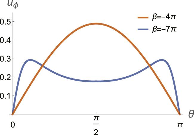
Figure 5. The velocity field uφ for the dipole state at a low energy (orange solid line) and at a high energy (blue solid line). The parameter region for the dipole state is $-8\pi ={\beta }_{s}^{d}\lt \beta \lt {\beta }_{c}^{d}\,=-4\pi $. When $\beta \to {\beta }_{s}^{d}$, uφ(θ = π/2) → 1/2π. Note that here the fluid velocity field on the northern hemisphere is obtained by shifting the coordinate of equation ( |
3.5. Comparison of the entropy between the sandwich state and the quadrupole state at high energies
The quadrupole state at high energies can be easily constructed from equations (78 ) and (79 ). From the approximate high-energy expressions of vortex densities, we can calculate the entropy and find again that S[sandwich state] > S[quadrupole state] (figure 6).
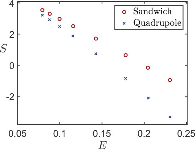
Figure 6. A comparison between the entropy of the sandwich state (red circle) and the quadrupole state (blue cross) at high energies. The entropy values are evaluated using equations ( |
3.6. Gaussian clustered states
In this section, we discuss a limit distribution when β → 0, ω → ∞ simultaneously while α = βω is finite. In this limit, equation (29 ) admits an exact solution:
$\begin{eqnarray}{n}_{\pm }(\theta )=\frac{\alpha }{4\pi \sinh \alpha }\exp (\mp \alpha \cos \theta ),\end{eqnarray}$
$\begin{eqnarray}\begin{array}{rcl}\psi (\theta ) & = & -\frac{1}{8\pi \sinh \alpha }\left[{{\rm{e}}}^{\alpha }{\rm{Ei}}\left(\alpha (\cos \theta -1)\right)-{{\rm{e}}}^{\alpha }{\rm{Ei}}\left(-\alpha (\cos \theta +1)\right)\right.\\ & & +{{\rm{e}}}^{-\alpha }{\rm{Ei}}\left(\alpha (1-\cos \theta )\right)-{{\rm{e}}}^{-\alpha }{\rm{Ei}}\left(\alpha (\cos \theta +1)\right)\\ & & \left.-2\alpha C\,{\rm{arctanh}}(\cos \theta )\right],\end{array}\end{eqnarray}$
where α ∈ (−∞, ∞), ${\rm{Ei}}(x)={\int }_{-\infty }^{x}{{\rm{e}}}^{t}/t\,{\rm{d}}t$, and C is a constant determined by proper smooth conditions. The angular momentum for this Gaussian state is $\begin{eqnarray}{L}_{\zeta }=\int ({n}_{+}-{n}_{-})\cos \theta \,{\rm{d}}{\rm{\Omega }}=\frac{2}{\alpha }(1-\alpha \coth \alpha ).\end{eqnarray}$
The components of the fluid velocity field for this state are uθ = 0 and
$\begin{eqnarray}{u}_{\phi }=-\frac{\partial \psi }{\partial \theta }=\frac{\alpha }{4\pi \sinh \alpha \sin \theta }\left[\frac{2\cosh (\alpha \cos \theta )}{\alpha }+C\right].\end{eqnarray}$
Here we impose the zero-velocity condition at poles, namely uφ(θ = 0) = uφ(θ = π) = 0, giving rise to $C=-2\cosh (\alpha )/\alpha $. figure 7 shows the vorticity distribution, the energy, and the angular momentum as functions of α. Note that the condition uφ(θ = π/2) = 0 leads to unphysical results uφ(θ = 0) = uφ(θ = π) = ∞ for α ≠ 0.
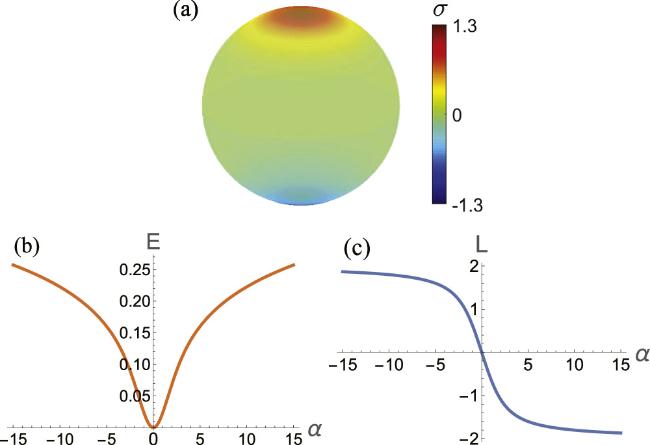
Figure 7. (a) Vorticity σ = n+ − n− for the Gaussian state at α = −8. (b) and (c) show the energy and the angular momentum of as functions of α, respectively. |
Similar to the fluid velocity field for the dipole state, for the Gaussian state the peak fluid velocity appears on the equator for small values of ∣α∣ and moves towards to poles as ∣α∣ exceeds a certain value of ∣αc∣ (figure 8), where ∣αc∣ satisfies ${{\alpha }_{c}}^{2}-\cosh ({\alpha }_{c})+1=0$. The amplitude of the fluid velocity on the equator is $| {u}_{\phi }(\theta =\pi /2)| =(1-1/\cosh \alpha )/(2\pi )$ and reaches the maximum value 1/2π when ∣α∣ → ∞.
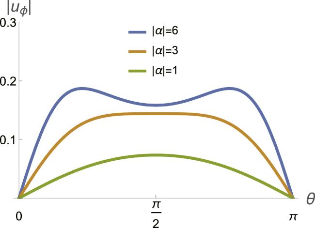
Figure 8. The amplitude of the fluid velocity field uφ for different values of ∣α∣. |
4. Monte Carlo simulations
In this section, we show numerical results from MC simulations of a large number of point vortices on a unit sphere. The simulations are performed for a range of increasing energies and at fixed angular momentum Lζ = 0 for the sandwich and quadrupole states and Lζ ≠ 0 for the dipole state.
4.1. Microcanonical Monte Carlo
In our microcanonical MC simulations, we adopt the general scheme developed in [12, 13, 24, 75], where the total energy E and the angular momentum Lζ are fixed within narrow shells. For vortices on a unit sphere, ${q}_{i}=\cos {\theta }_{i}$ and pi = φi are canonical variables [48]. In order to keep sampling vortices uniform in the phase space, at each MC step, we randomly choose a vortex dipole at positions r+(θi, φi) and r−(θi, φi) and move it to ${{\boldsymbol{r}}}^{{+}}({\theta }_{i}^{{\prime} },{\phi }_{i}^{{\prime} })$ and ${{\boldsymbol{r}}}^{{-}}({\theta }_{i}^{{\prime} },{\phi }_{i}^{{\prime} })$, where ${\phi }^{{\prime} }=p$, ${\theta }_{i}^{{\prime} }=\arccos (q)$ with p ∈ [0, 2π] and q ∈ [−1, 1] being independent and uniformly distributed random variables. The new configuration is accepted if the updated energy ${E}^{{\prime} }$ and the updated angular momentum ${L}_{\zeta }^{{\prime} }$ are within the narrow shells. Otherwise, the vortex configuration remains the same as the previous one.
4.2. The sandwich state versus the quadrupole state
By appropriately choosing initial vortex distributions for given energies and zero angular momentum, the sandwich state appears at the end of our MC sampling. Comparisons between the analytical predictions and the numerical results is shown in figure 9 and excellent agreements are found. Caution should be taken here, as the initial configurations are chosen to close to the sandwich state due to our limited MC sampling efficiency. It is difficult for our current MC sampling method to select the sandwich state, but not the quadrupole state, from a random initial vortex distribution within the energy and angular momentum constraints.
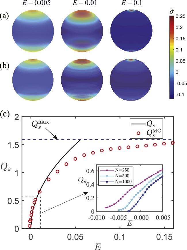
Figure 9. A comparison between the mean-field theory and MC simulations for N = 1000 point vortices. (a) and (b) show results from the mean-field theory and MC sampling for the scaled vorticity $\tilde{\sigma }$, respectively. Here $\tilde{\sigma }=\sigma $ for E = 0.005, E = 0.01, and $\tilde{\sigma }=\sigma /10$ for E = 0.1. The reason for introducing the scaled vorticity $\tilde{\sigma }$ is to present the large energy range on a single color map. (c) The quadrupole moment Qs for increasing energy E (circle red) and the mean-field prediction equation ( |
To verify that the sandwich state is the maximum entropy state for large but finite N, we numerically evaluate the entropy values of the sandwich state and the quadrupole state at a certain energy range. The entropy values are evaluated using equation (17 ). We uniformly divide the phase space of a vortex on a unit sphere into a large number of cells labeled by [qi, pj] with ${q}_{i}=-1+2(i-1)/\tilde{N}$, ${p}_{j}=2\pi (j-1)/\tilde{N}$, and $i,j=1,...\tilde{N}+1$, where (i, j) denotes the cell index and ${\tilde{N}}^{2}$ is number of the cells. The area of a cell is then ${a}_{i}=4\pi /{\tilde{N}}^{2}$. In terms of spherical coordinates, the cell labels are [θi, φi] with ${\theta }_{i}=\arccos \,{q}_{i}$ and φj = pi. Note that here $\tilde{N}$ should be properly chosen such that most cells contain a sufficient large number of vortices. Using this method, we confirm that the sandwich state has higher entropy than the quadrupole state (figure 10).
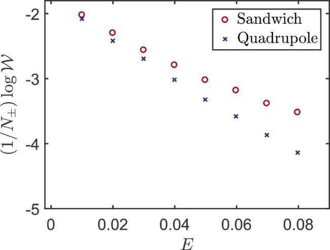
Figure 10. A comparison between the entropy of the quadrupole state and the sandwich state. Here $\tilde{N}=32$ and the quadrupole and the sandwich states are prepared via MC sampling for N = 4000 point vortices with initial vortex distributions very closed to the quadrupole state and the sandwich state, respectively. The entropy is negative because of the artificial choice of the minimum area in the phase space, and only the entropy difference between the two states has physical meaning. |
4.3. The dipole state
Our perturbation analysis at low energies (section 3.3.1 ) shows that for Lζ ≠ 0 and ω = 0 the dipole state maximizes the entropy for a neutral vortex system on a sphere. This is different from neutral vortices confined to a disc where the dipole state carries zero angular momentum [24]. In this subsection, we present the MC simulations and compare them with our analytical predictions, showing excellent agreements (figure 11).
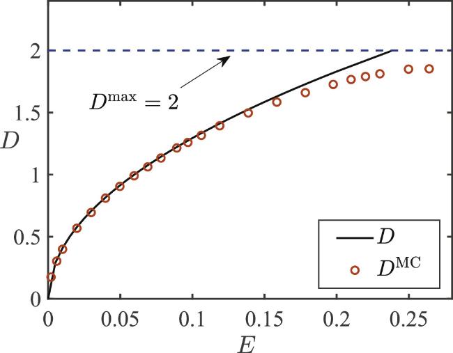
Figure 11. A comparison between the analytical prediction $D=| {D}_{\zeta }| =4\sqrt{\pi /3}\sqrt{E}$ [equation ( |
5. Conclusion and discussion
We investigate rotation-free Onsager vortex clustered states of point vortices confined on a sphere. We find that the sandwich state is the most probable state with zero angular momentum and is characterized by the quadrupole moment tensor. The dipole state is the maximum entropy state with finite angular momentum and is characterized by nonzero dipole moment. Our mean-field analytical predictions agree well with the results of MC simulations. In [31], it is shown that the point-vortex dynamics combined with removing low-energy vortex pairs drives an initial uniform vortex state to the quadruple state. Since the quadruple distribution also solves the self-consistent equation, it is a local maximum entropy state. In the situation described in [31], vortices may be dynamically trapped in this local equilibrium state. Exploring the entropy barrier between the sandwich state and the quadruple state, and its effect on the dynamical transitions between the two states, deserves further investigations.