


1. Introduction
In recent years, there has been expanding attention toward quantum thermodynamic research through quantum resources. Quantum resource theories (QRT) [1] provide a rigorous and general framework to study various and different quantum phenomena in quantum mechanics. With the advancement of quantum information technology, quantum resources including quantum coherence [2–4] and quantum correlations [5–7], along with quantum control strategies, have emerged as a prominent research focus in quantum thermodynamics. In addition to the quantum resources, many other quantum traits and strategies such as the environmental memory effect (non-Markovianity) [8, 9] and noise-induced interference within shared environments [10, 11] have been demonstrated to thermodynamics.
Quantum coherence and correlations have been extensively applied in quantum technologies to achieve various schemes that are otherwise unfeasible only by means of classical resources. It was shown that the coherence and correlation can be exploited to improve the performance and/or the power of thermal machines [12], to enhance work extraction from a quantum system [13] and to increase the system’s thermalization temperature [14]. It is emphasized that quantum coherence rather than quantum correlations can reflect the effects of the reservoir on the system’s work capability effectively [15, 16]. The role of coherences and correlations in Landauer’s Principle have also been studied [17, 18]. Subsequently, extensive research has focused on the utilization of quantum coherence and quantum correlations in optimizing the design and performance of quantum thermal devices [19], facilitating work extraction processes [20], and elevating the operational thermalization temperature thresholds in quantum systems [21, 22].
Due to the well-known advantages of quantum over conventional computers, it is natural to wonder whether coherence effects might be able to enhance thermal machines similarly. The phenomenon of quantum coherence was systematically examined through a theoretical investigation of the photo-Carnot engine [23], a thermodynamic framework featuring a working medium constituted by a four-level quantum system. Pioneering research conducted by Scully et al established that operational efficiency enhancement could be attained through non-equilibrium state preparation facilitated by coherent thermal reservoirs, with the realized efficiency exceeding the classical Carnot thermodynamic efficiency limit [24]. The advantage of quantum coherence in driving engines has been experimentally realized in the platform of nitrogen vacancy centers in diamond [25]. Most recently the thermodynamic effects of quantum coherence have attracted much attention as a promising candidate for designing thermal machines. Many interesting investigations have been performed in various systems and models, such as quantum optical systems including microwave cavities [26], ion traps [27], optical lattices [28], optomechanical systems [29], and biological systems [30]. Nevertheless, how to quantify the role of quantum coherence in thermodynamics with a general approach remains an open problem, despite substantial progress through case-specific investigations [31, 32].
The fundamental significance of quantum coherences in the realm of quantum thermodynamics has been garnered through a growing number of practical applications including quantum thermal machines. Study of coupled quantum systems as quantum heat engines is an interesting research area. The quantum systems with quantum coherence are generally served as the working substance of quantum engines or thermodynamic cycles, i.e., the coherence come from the working substance of quantum engines. Coherence in system-bath interactions that originates from the interference may enhance the power [33, 34] and efficiency [35]. So far, many quantum coherence effects have been studied in continuously working bosonic devices [33–36]. Notably, coupled systems as heat engine [37–39], heat pump [40], and multitask thermal machine can be driven by pure quantum coherence [41]. It has been shown that appropriate coupling can increase the efficiency of the system compared to the uncoupled model [42, 43].
Motivated by recent advancements in experimental techniques for the manipulation of single or few-body quantum systems [44], a thermodynamic description of microscale and nanoscale phenomena has been attracting a huge deal of attention [45]. The dipole-dipole interaction (DDI) between atoms is one of the most important features for the many-atom system. It is the cause of the van der Waals attraction which plays a considerable role in various chemical physics processes [46–48]. In fact, the dipole-dipole interaction (DDI) can profoundly affect the light absorption characteristics and lead to a shift of the atomic energy levels [49]. In recent years, substantial progress has been made on solid materials [50, 51] and ultracold atoms [52, 53]. Motivated by these works, the present work is an attempt to use a pair of a system of two dipole-dipole coupled two-level atoms in a cavity as working substance for the quantum Otto cycle.
The remainder of the paper is structured as follows. In section 2 , we present the model of two coupled two-level atoms system and obtain the eigenvalues and corresponding eigenstates. In section 3 , we introduce the general QOE theories. In section 4 , we study the relation between thermodynamics and quantum coherence. In section 5 , we provide a discussion of the results. In section 6 , we analysis the relations between local and global efficiency. Finally, some conclusions are given.
2. Description of physical model
We consider a pair of two-level atoms labeled A and B with ground states $\left|g\right\rangle $ and excited states $\left|e\right\rangle $ (see figure 1). The Hamiltonian for the total system reads [54, 55]
$\begin{eqnarray}\begin{array}{r}\hat{{ \mathcal H }}\,=\,\frac{\hslash }{2}\left({\omega }_{{\rm{A}}}{\hat{\sigma }}_{{\rm{A}}}^{z}\displaystyle \otimes {\hat{\sigma }}_{0}+{\omega }_{{\rm{B}}}{\hat{\sigma }}_{0}\displaystyle \otimes {\hat{\sigma }}_{{\rm{B}}}^{z}\right)\\ \,+\,\hslash {\rm{\Omega }}\left({\hat{\sigma }}_{{\rm{A}}}^{-}\displaystyle \otimes {\hat{\sigma }}_{{\rm{B}}}^{+}+{\hat{\sigma }}_{{\rm{A}}}^{+}\displaystyle \otimes {\hat{\sigma }}_{{\rm{B}}}^{-}\right),\end{array}\end{eqnarray}$
where ${\hat{\sigma }}_{i}^{z}=\left|{e}_{i}\right\rangle \left\langle {e}_{i}\right|-\left|{g}_{i}\right\rangle \left\langle {g}_{i}\right|$ is the energy operator, ${\hat{\sigma }}_{i}^{+}=\left|{e}_{i}\right\rangle \left\langle {g}_{i}\right|$ and ${\hat{\sigma }}_{i}^{-}=\left|{g}_{i}\right\rangle \left\langle {e}_{i}\right|$ are the dipole raising and lowering operators, ωi is the atomic transition frequency of the ith $\left(i={\rm{A}},{\rm{B}}\right)$ atom. The second term represents the dipole-dipole Van der Waals coupling between the atoms and Ω is the coupling constant of the dipole interaction.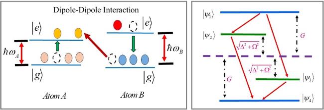
Figure 1. Schematic energy level diagram of two coupled two-level atoms in thermal equilibrium and the equivalent four-level system. Here label $g\left(e\right)$ indicates ground (excited) state. |
In the basis of the product states $\left\{\left|ee\right\rangle ,\left|eg\right\rangle ,\left|ge\right\rangle ,\left|gg\right\rangle \right\}$, the Hamiltonian (1 ) can be written in a matrix form as
$\begin{eqnarray}\hat{{ \mathcal H }}=\left(\begin{array}{cccc}{ \mathcal G } & 0 & 0 & 0\\ 0 & {\rm{\Delta }} & {\rm{\Omega }} & 0\\ 0 & {\rm{\Omega }} & -{\rm{\Delta }} & 0\\ 0 & 0 & 0 & -{ \mathcal G }\end{array}\right),\end{eqnarray}$
where ${ \mathcal G }=\frac{\hslash }{2}\left({\omega }_{{\rm{A}}}+{\omega }_{{\rm{B}}}\right)$ represents the average frequency of atomic transition frequencies, and ${\rm{\Delta }}=\frac{\hslash }{2}\left({\omega }_{{\rm{A}}}-{\omega }_{{\rm{B}}}\right)$ denotes the frequency detuning arising from dipole-dipole interactions.The eigenvalues can be readily evaluated as
$\begin{eqnarray}\begin{array}{l}{E}_{1}={ \mathcal G },\\ {E}_{2}=\sqrt{{{\rm{\Delta }}}^{2}+{{\rm{\Omega }}}^{2}},\\ {E}_{3}=-\sqrt{{{\rm{\Delta }}}^{2}+{{\rm{\Omega }}}^{2}},\\ {E}_{4}=-{ \mathcal G },\end{array}\end{eqnarray}$
and the corresponding eigenvectors are given by $\begin{eqnarray}\begin{array}{l}\left|{\psi }_{1}\right\rangle =\left|ee\right\rangle ,\\ \left|{\psi }_{2}\right\rangle =\frac{1}{\sqrt{1+{\eta }_{+}^{2}}}\left({\eta }_{+}\left|ge\right\rangle +\left|eg\right\rangle \right),\\ \left|{\psi }_{3}\right\rangle =\frac{1}{\sqrt{1+{\eta }_{-}^{2}}}\left({\eta }_{-}\left|ge\right\rangle +\left|eg\right\rangle \right),\\ \left|{\psi }_{4}\right\rangle =\left|gg\right\rangle ,\end{array}\end{eqnarray}$
with ${\eta }_{\pm }=\frac{{\rm{\Delta }}\pm \sqrt{{{\rm{\Delta }}}^{2}+{{\rm{\Omega }}}^{2}}}{{\rm{\Omega }}}$.3. General quantum Otto engine
We study the QOE operating under a four-stroke cycle. This cycle is composed of two quantum isochoric processes (stages 1 and 3) and two quantum adiabatic processes (stages 2 and 4). The working substance interacts with a cold (hot) reservoir at temperature ${{ \mathcal T }}_{{\rm{l}}}\left({{ \mathcal T }}_{{\rm{h}}}\right)$. We will consider that the dipole-dipole interaction coupling strength Ω is kept constant throughout the cycle. The thermodynamic cycle is shown in figure 1 and proceeds is described as follows.
Stage 1: Quantum isochoric process (hot bath stage). The system prepared in the initial state is connected to a hot thermal reservoir at temperature ${{ \mathcal T }}_{{\rm{h}}}$ until it reaches thermal equilibrium with average frequency ${{ \mathcal G }}_{{\rm{h}}}$. In the isochoric process, the population of the four discrete level is changing from the population pil, (i = 1, 2, 3, 4) to the population pih, (i = 1, 2, 3, 4) and only heat is transferred to yield a change in the occupation probabilities, and there is no change in the values of the energy levels.
$\begin{eqnarray}\begin{array}{l}{p}_{1{\rm{h}}}=\frac{1}{{Z}_{{\rm{h}}}}{\rm{\exp }}\left(-{\beta }_{{\rm{h}}}{{ \mathcal G }}_{{\rm{h}}}\right),{p}_{2{\rm{h}}}=\frac{1}{{Z}_{{\rm{h}}}}{\rm{\exp }}\left(-{\beta }_{{\rm{h}}}\sqrt{{{\rm{\Delta }}}^{2}+{{\rm{\Omega }}}^{2}}\right),\\ {p}_{3{\rm{h}}}=\frac{1}{{Z}_{{\rm{h}}}}{\rm{\exp }}\left({\beta }_{{\rm{h}}}\sqrt{{{\rm{\Delta }}}^{2}+{{\rm{\Omega }}}^{2}}\right),{p}_{4{\rm{h}}}=\frac{1}{{Z}_{{\rm{h}}}}{\rm{\exp }}\left({\beta }_{{\rm{h}}}{{ \mathcal G }}_{{\rm{h}}}\right),\end{array}\end{eqnarray}$
and $\begin{eqnarray}\begin{array}{l}{p}_{1{\rm{l}}}=\frac{1}{{Z}_{{\rm{l}}}}{\rm{\exp }}\left(-{\beta }_{{\rm{l}}}{{ \mathcal G }}_{l}\right),{p}_{2{\rm{l}}}=\frac{1}{{Z}_{l}}{\rm{\exp }}\left(-{\beta }_{{\rm{l}}}\sqrt{{{\rm{\Delta }}}^{2}+{{\rm{\Omega }}}^{2}}\right),\\ {p}_{3{\rm{l}}}=\frac{1}{{Z}_{{\rm{l}}}}{\rm{\exp }}\left({\beta }_{{\rm{l}}}\sqrt{{{\rm{\Delta }}}^{2}+{{\rm{\Omega }}}^{2}}\right),{p}_{4{\rm{l}}}=\frac{1}{{Z}_{{\rm{l}}}}{\rm{\exp }}\left({\beta }_{{\rm{l}}}{{ \mathcal G }}_{{\rm{l}}}\right),\end{array}\end{eqnarray}$
where $\begin{eqnarray}{{ \mathcal Z }}_{{\rm{h}}}=2\left[\cosh \left({\beta }_{{\rm{h}}}{{ \mathcal G }}_{{\rm{h}}}\right)+\cosh \left({\beta }_{{\rm{h}}}\sqrt{{{\rm{\Delta }}}^{2}+{{\rm{\Omega }}}^{2}}\right)\right],\end{eqnarray}$
and $\begin{eqnarray}{{ \mathcal Z }}_{{\rm{l}}}=2\left[\cosh \left({\beta }_{{\rm{l}}}{{ \mathcal G }}_{{\rm{l}}}\right)+\cosh \left({\beta }_{{\rm{l}}}\sqrt{{{\rm{\Delta }}}^{2}+{{\rm{\Omega }}}^{2}}\right)\right].\end{eqnarray}$
Stage 2: Quantum adiabatic (expansion) process. The average frequency of the working medium is changed from ${{ \mathcal G }}_{{\rm{h}}}$ to ${{ \mathcal G }}_{{\rm{l}}}\quad \left({{ \mathcal G }}_{{\rm{l}}}\lt {{ \mathcal G }}_{{\rm{h}}}\right)$, provided the expansion rate is sufficiently slow according to the quantum adiabatic theorem. During this process, the occupation probability pih, (i = 1, 2, 3, 4) is kept fixed. The working medium is decoupled from the hot reservoir, and the energy structure is varied from Eih, (i = 1, 2, 3, 4) to Eil, (i = 1, 2, 3, 4). The engine performs an amount of positive work when the energy spacings decrease.
$\begin{eqnarray}\begin{array}{rcl}{E}_{1{\rm{h}}} & = & {{ \mathcal G }}_{{\rm{h}}},{E}_{2{\rm{h}}}=\sqrt{{{\rm{\Delta }}}^{2}+{{\rm{\Omega }}}^{2}},\\ {E}_{3{\rm{h}}} & = & -\sqrt{{{\rm{\Delta }}}^{2}+{{\rm{\Omega }}}^{2}},{E}_{4{\rm{h}}}=-{{ \mathcal G }}_{{\rm{h}}},\end{array}\end{eqnarray}$
and $\begin{eqnarray}\begin{array}{rcl}{E}_{1{\rm{l}}} & = & {{ \mathcal G }}_{{\rm{l}}},{E}_{2{\rm{l}}}=\sqrt{{{\rm{\Delta }}}^{2}+{{\rm{\Omega }}}^{2}},\\ {E}_{3{\rm{l}}} & = & -\sqrt{{{\rm{\Delta }}}^{2}+{{\rm{\Omega }}}^{2}},{E}_{4{\rm{l}}}=-{{ \mathcal G }}_{{\rm{l}}}.\end{array}\end{eqnarray}$
Stage 3: Quantum isochoric process (cold bath stage). Stage 3 is almost an inverse process of Stage 1. The working substance with average frequency ${{ \mathcal G }}_{{\rm{l}}}$ is coupled to a cold reservoir of temperature ${{ \mathcal T }}_{{\rm{l}}}$ and its energy structure is kept fixed. The population of the four discrete level is changing from the initial population pih, (i = 1, 2, 3, 4) to population pil, (i = 1, 2, 3, 4) and some heat is thus transferred but no work is performed in this stage.
Stage 4: Quantum adiabatic (compression) process. The system is isolated from the cold reservoir and the average frequency is changed from ${{ \mathcal G }}_{{\rm{l}}}$ to ${{ \mathcal G }}_{{\rm{h}}}$. During this process the populations pil, (i = 1, 2, 3, 4) remain constant while the energy structure is varied from Eil, (i = 1, 2, 3, 4) to Eih, (i = 1, 2, 3, 4). In this stage an amount of work is done on the system.
The expectation value of the system is
$\begin{eqnarray}{ \mathcal U }=\left\langle E\right\rangle =\displaystyle \sum _{j={\rm{h}},{\rm{l}}}\displaystyle \sum _{i=1,}^{4}{p}_{ij}{E}_{ij},\end{eqnarray}$
in which Eij, (i = 1, 2, 3, 4; j = h, l) are the energy levels and pij, (i = 1, 2, 3, 4; j = h, l) are the corresponding occupation probabilities. Infinitesimally, $\begin{eqnarray}{\rm{d}}{ \mathcal U }=\displaystyle \sum _{j={\rm{h}},{\rm{l}}}\displaystyle \sum _{i=1}^{4}{E}_{ij}{\rm{d}}{p}_{ij}+{p}_{ij}{\rm{d}}{E}_{ij},\end{eqnarray}$
from which we make the following identifications for infinitesimal heat transferred $d{ \mathcal Q }$ and work done $d{ \mathcal W }$. $\begin{eqnarray}{\rm{d}}{ \mathcal Q }=\displaystyle \sum _{j={\rm{h}},{\rm{l}}}\displaystyle \sum _{i=1}^{4}{E}_{ij}{\rm{d}}{p}_{ij},{\rm{d}}{ \mathcal W }=\displaystyle \sum _{j={\rm{h}},{\rm{l}}}\displaystyle \sum _{i=1}^{4}{p}_{ij}{\rm{d}}{E}_{ij}.\end{eqnarray}$
4. Relation between thermodynamics and quantum coherence
The state of two coupled two-level atoms interacting with the environmental thermal reservoir under the thermal equilibrium conditions is described by
$\begin{eqnarray}\hat{\varrho }\left({ \mathcal T }\right)=\frac{1}{{ \mathcal Z }}{\rm{\exp }}\left(-\beta \hat{{ \mathcal H }}\right),\end{eqnarray}$
in which the partition function is ${ \mathcal Z }$ = $Tr\left[\exp \left(-\hat{{ \mathcal H }}/{k}_{{\rm{B}}}{ \mathcal T }\right)\right]$, kB is the Boltzmann’s constant and ${ \mathcal T }$ is the temperature. The thermal density matrix of the system in the standard basis $\left\{\left|ee\right\rangle ,\left|eg\right\rangle ,\left|ge\right\rangle ,\left|gg\right\rangle \right\}$ takes the following form $\begin{eqnarray}\hat{\varrho }=\left(\begin{array}{cccc}{p}_{1} & 0 & 0 & 0\\ 0 & \frac{1+{\rm{\Gamma }}}{2}{p}_{2}+\frac{1-{\rm{\Gamma }}}{2}{p}_{3} & \frac{{\rm{\Lambda }}}{2}\left({p}_{2}-{p}_{3}\right) & 0\\ 0 & \frac{{\rm{\Lambda }}}{2}\left({p}_{2}-{p}_{3}\right) & \frac{1-{\rm{\Gamma }}}{2}{p}_{2}+\frac{1+{\rm{\Gamma }}}{2}{p}_{3} & 0\\ 0 & 0 & 0 & {p}_{4}\end{array}\right).\end{eqnarray}$
The occupation probabilities of the system in the thermal state at temperature ${ \mathcal T }$ are given by
$\begin{eqnarray}\begin{array}{rcl}{p}_{1} & = & \frac{1}{{ \mathcal Z }}{{\rm{e}}}^{-\beta { \mathcal G }},{p}_{2}=\frac{1}{{ \mathcal Z }}{{\rm{e}}}^{-\beta \sqrt{{{\rm{\Delta }}}^{2}+{{\rm{\Omega }}}^{2}}},\\ {p}_{3} & = & \frac{1}{{ \mathcal Z }}{{\rm{e}}}^{\beta \sqrt{{{\rm{\Delta }}}^{2}+{{\rm{\Omega }}}^{2}}},{p}_{4}=\frac{1}{{ \mathcal Z }}{{\rm{e}}}^{\beta { \mathcal G }},\end{array}\end{eqnarray}$
where the partition function ${ \mathcal Z }$ = $2\left[\cosh \left(\beta G\right)\right.$ + $\left.\cosh \left(\beta \sqrt{{{\rm{\Delta }}}^{2}+{{\rm{\Omega }}}^{2}}\right)\right]$, ${\rm{\Gamma }}=\frac{{\rm{\Delta }}}{\sqrt{{{\rm{\Delta }}}^{2}+{{\rm{\Omega }}}^{2}}}$ and ${\rm{\Lambda }}=\frac{{\rm{\Omega }}}{\sqrt{{{\rm{\Delta }}}^{2}+{{\rm{\Omega }}}^{2}}}$.To quantify the coherence of two coupled two-level atoms, we focus on the off-diagonal elements of $\hat{\varrho }$ in the basis $\left\{\left|ee\right\rangle ,\left|eg\right\rangle ,\left|ge\right\rangle ,\left|gg\right\rangle \right\}$. The l1 norm of quantum coherence is defined as [56, 57]
$\begin{eqnarray}{{ \mathcal C }}_{{l}_{1}}\left({\hat{\varrho }}_{{\rm{AB}}}\right)=\displaystyle \sum _{i\ne j}\left|{\hat{\varrho }}_{i,j}\right|.\end{eqnarray}$
The non-diagonal (diagonal) elements ${\hat{\varrho }}_{ij,i\ne j}\left({\hat{\varrho }}_{ij,i=j}\right)$ represent the atomic coherences (populations). We can obtain the l1 norm of coherence ${{ \mathcal C }}_{{l}_{1}}$ as follows
$\begin{eqnarray}{{ \mathcal C }}_{{l}_{1}}=2\left|\hat{{\varrho }_{23}}\right|={\rm{\Lambda }}\left|{p}_{2}-{p}_{3}\right|={\rm{\Lambda }}\left({p}_{3}-{p}_{2}\right).\end{eqnarray}$
The value ${{ \mathcal C }}_{{l}_{1}}$ verifies the uniformity for all quantum states. Substituting equation (16 ) in to equation (18 ), l1 norm of coherence ${{ \mathcal C }}_{{l}_{1}}$ can be expressed as
$\begin{eqnarray}{{ \mathcal C }}_{{l}_{1}}=\frac{{\rm{\Lambda }}\sinh \left(\beta \sqrt{{{\rm{\Delta }}}^{2}+{{\rm{\Omega }}}^{2}}\right)}{\cosh \left(\beta { \mathcal G }\right)+\cosh \left(\beta \sqrt{{{\rm{\Delta }}}^{2}+{{\rm{\Omega }}}^{2}}\right)}.\end{eqnarray}$
The critical quantum coherence is exclusively determined by the coupling strength in the case of identical $\left({\rm{\Delta }}=0\right)$ as well as non-identical atoms $\left({\rm{\Delta }}\ne 0\right)$.
The quantum coherence under our consideration is that of two thermal equilibrium states at the end of stage 1 and stage 3, denoted by ${{ \mathcal C }}_{{l}_{1}{\rm{h}}}$ and ${{ \mathcal C }}_{{l}_{1}{\rm{l}}}$, respectively. They are given by
$\begin{eqnarray}{{ \mathcal C }}_{{l}_{1}{\rm{h}}}=\frac{{\rm{\Lambda }}\sinh \left({\beta }_{{\rm{h}}}\sqrt{{{\rm{\Delta }}}^{2}+{{\rm{\Omega }}}^{2}}\right)}{\cosh \left({\beta }_{{\rm{h}}}{{ \mathcal G }}_{{\rm{h}}}\right)+\cosh \left({\beta }_{{\rm{h}}}\sqrt{{{\rm{\Delta }}}^{2}+{{\rm{\Omega }}}^{2}}\right)},\end{eqnarray}$
$\begin{eqnarray}{{ \mathcal C }}_{{l}_{1}{\rm{l}}}=\frac{{\rm{\Lambda }}\sinh \left({\beta }_{{\rm{l}}}\sqrt{{{\rm{\Delta }}}^{2}+{{\rm{\Omega }}}^{2}}\right)}{\cosh \left({\beta }_{{\rm{l}}}{{ \mathcal G }}_{{\rm{l}}}\right)+\cosh \left({\beta }_{{\rm{l}}}\sqrt{{{\rm{\Delta }}}^{2}+{{\rm{\Omega }}}^{2}}\right)}.\end{eqnarray}$
It is evident that in the absence of the dipole-dipole interaction (Ω = 0), quantum coherence ${{ \mathcal C }}_{{l}_{1}{\rm{h}}}$ and ${{ \mathcal C }}_{{l}_{1}{\rm{l}}}$ completely vanishes for all values of the average frequency ${{ \mathcal G }}_{{\rm{h}}}\left({{ \mathcal G }}_{{\rm{l}}}\right)$ in the system.
For comparison, we visually depict the quantum coherence ${{ \mathcal C }}_{{l}_{1}{\rm{h}}}\left({{ \mathcal C }}_{{l}_{1}{\rm{l}}}\right)$ as a function of the average frequency ${{ \mathcal G }}_{{\rm{h}}}\left({{ \mathcal G }}_{{\rm{l}}}\right)$ with fixed parameters ${{ \mathcal T }}_{{\rm{h}}}=10.0$, ${{ \mathcal T }}_{{\rm{l}}}=5.0$ and kB = 1 using the analytical results derived from equations (20 ) and (21 ) as shown in figure 2. We can see that quantum coherence ${{ \mathcal C }}_{{l}_{1}{\rm{h}}}\left({{ \mathcal C }}_{{l}_{1}{\rm{l}}}\right)$ decreases with the average frequency ${{ \mathcal G }}_{{\rm{h}}}\left({{ \mathcal G }}_{{\rm{l}}}\right)$ monotonously and vanishes in the case of higher the average frequency ${{ \mathcal G }}_{{\rm{h}}}\left({{ \mathcal G }}_{{\rm{l}}}\right)$ as expected. Furthermore, from these curves, it is evident that quantum coherence ${{ \mathcal C }}_{{l}_{1}{\rm{h}}}\left({{ \mathcal C }}_{{l}_{1}{\rm{l}}}\right)$ can be enhanced by increasing the coupling constant $\left({\rm{\Omega }}\right)$ or reducing the frequency detuning. We note that, for small values of frequency detuning $\left({\rm{\Delta }}\right)$, the variations of quantum coherence ${{ \mathcal C }}_{{l}_{1}{\rm{h}}}\left({{ \mathcal C }}_{{l}_{1}{\rm{l}}}\right)$ displays a rapid decrease from a maximum value ${{ \mathcal C }}_{{l}_{1}{\rm{h}},{\rm{m}}{\rm{a}}{\rm{x}}}\left({{ \mathcal C }}_{{l}_{1}{\rm{l}},{\rm{m}}{\rm{a}}{\rm{x}}}\right)$ to zero when the interatomic dipole coupling strength $\left({\rm{\Omega }}\right)$ attains criticality. The analysis demonstrates that frequency detuning induces system decoherence through the disruption of coherent energy exchange.
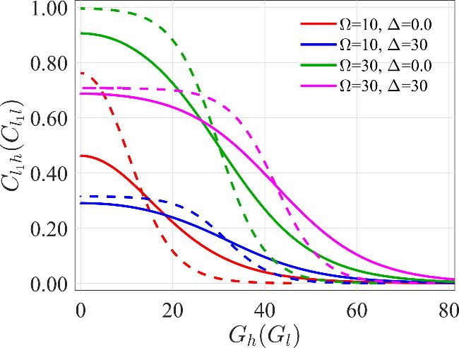
Figure 2. The l1 norm of quantum coherence ${{ \mathcal C }}_{{l}_{1}{\rm{h}}}$ (solid line) versus the average frequency ${{ \mathcal G }}_{{\rm{h}}}$ and quantum coherence ${{ \mathcal C }}_{{l}_{1}{\rm{l}}}$ ( dashed line) versus the average frequency ${{ \mathcal G }}_{{\rm{l}}}$ of a pair of atoms system. The parameters are ${{ \mathcal T }}_{{\rm{h}}}=10.0$, ${{ \mathcal T }}_{{\rm{l}}}=5.0$ and kB = 1. |
5. Results and discussion
5.1. Case One: without the presence of the dipole-dipole interaction, i.e. Ω = 0
When there are no dipole-dipole interactions, i.e., Ω = 0, two atoms are independent of each other. Based on equations (20 ) and (21 ), quantum coherence of the system can be described as
$\begin{eqnarray}{{ \mathcal C }}_{{l}_{1}{\rm{h}}}=0,{{ \mathcal C }}_{{l}_{1}{\rm{l}}}=0.\end{eqnarray}$
(a) Two Identical Atoms, i.e. Δ = 0.
Using equation (19 ), The heat transferred in Stage 1 and in Stage 3 of the cycle respectively is
$\begin{eqnarray}{{ \mathcal Q }}_{{\rm{h}}}=\left[-\tanh \left({\beta }_{{\rm{h}}}{{ \mathcal G }}_{{\rm{h}}}/2\right)+\tanh \left({\beta }_{{\rm{l}}}{{ \mathcal G }}_{{\rm{l}}}/2\right)\right]{{ \mathcal G }}_{{\rm{h}}},\end{eqnarray}$
and $\begin{eqnarray}{{ \mathcal Q }}_{{\rm{l}}}=\left[\tanh \left({\beta }_{{\rm{h}}}{{ \mathcal G }}_{{\rm{h}}}/2\right)-\tanh \left({\beta }_{{\rm{l}}}{{ \mathcal G }}_{{\rm{l}}}/2\right)\right]{{ \mathcal G }}_{{\rm{l}}}.\end{eqnarray}$
The work done in Stage 2 and Stage 4 by the QOE as
$\begin{eqnarray}{ \mathcal W }=\left(-{{ \mathcal G }}_{{\rm{h}}}+{{ \mathcal G }}_{{\rm{l}}}\right)\left[\tanh \left({\beta }_{{\rm{h}}}{{ \mathcal G }}_{{\rm{h}}}/2\right)-\tanh \left({\beta }_{{\rm{l}}}{{ \mathcal G }}_{{\rm{l}}}/2\right)\right],\end{eqnarray}$
and the efficiency reads $\begin{eqnarray}\eta ={\eta }_{0}=1-{{ \mathcal G }}_{{\rm{l}}}/{{ \mathcal G }}_{{\rm{h}}},\end{eqnarray}$
where η0 is the efficiency of the two identical two-level atoms in the absence of the dipole coupling strength Ω = 0.(b) Non-identical Atoms, i.e. Δ ≠ 0.
The heat transferred in Stage 1 and in Stage 3 of the cycle respectively is
$\begin{eqnarray}\begin{array}{rcl}{{ \mathcal Q }}_{{\rm{h}}} & = & \left(-\frac{\sinh \left({\beta }_{{\rm{h}}}{\rm{\Delta }}\right)}{\cosh \left({\beta }_{{\rm{h}}}{\rm{\Delta }}\right)+\cosh \left({\beta }_{{\rm{h}}}{{ \mathcal G }}_{{\rm{h}}}\right)}\right.\\ & & \left.+\frac{\sinh \left({\beta }_{{\rm{l}}}{\rm{\Delta }}\right)}{\cosh \left({\beta }_{{\rm{l}}}{\rm{\Delta }}\right)+\cosh \left({\beta }_{{\rm{l}}}{{ \mathcal G }}_{{\rm{l}}}\right)}\right){\rm{\Delta }}\\ & & +\left(-\frac{\sinh \left({\beta }_{{\rm{h}}}{{ \mathcal G }}_{{\rm{h}}}\right)}{\cosh \left({\beta }_{{\rm{h}}}{\rm{\Delta }}\right)+\cosh \left({\beta }_{{\rm{h}}}{{ \mathcal G }}_{{\rm{h}}}\right)}\right.\\ & & \left.+\frac{\sinh \left({\beta }_{{\rm{l}}}{{ \mathcal G }}_{{\rm{l}}}\right)}{\cosh \left({\beta }_{{\rm{l}}}{\rm{\Delta }}\right)+\cosh \left({\beta }_{{\rm{l}}}{{ \mathcal G }}_{{\rm{l}}}\right)}\right){{ \mathcal G }}_{{\rm{h}}},\end{array}\end{eqnarray}$
and $\begin{eqnarray}\begin{array}{rcl}{{ \mathcal Q }}_{{\rm{l}}} & = & \left(\frac{\sinh \left({\beta }_{{\rm{h}}}{\rm{\Delta }}\right)}{\cosh \left({\beta }_{{\rm{h}}}{\rm{\Delta }}\right)+\cosh \left({\beta }_{{\rm{h}}}{{ \mathcal G }}_{{\rm{h}}}\right)}\right.\\ & & \left.-\frac{\sinh \left({\beta }_{{\rm{l}}}{\rm{\Delta }}\right)}{\cosh \left({\beta }_{{\rm{l}}}{\rm{\Delta }}\right)+\cosh \left({\beta }_{{\rm{l}}}{{ \mathcal G }}_{{\rm{l}}}\right)}\right){\rm{\Delta }}\\ & & +\left(\frac{\sinh \left({\beta }_{{\rm{h}}}{{ \mathcal G }}_{{\rm{h}}}\right)}{\cosh \left({\beta }_{{\rm{h}}}{\rm{\Delta }}\right)+\cosh \left({\beta }_{{\rm{h}}}{{ \mathcal G }}_{{\rm{h}}}\right)}\right.\\ & & \left.-\frac{\sinh \left({\beta }_{{\rm{l}}}{{ \mathcal G }}_{{\rm{l}}}\right)}{\cosh \left({\beta }_{{\rm{l}}}{\rm{\Delta }}\right)+\cosh \left({\beta }_{{\rm{l}}}{{ \mathcal G }}_{{\rm{l}}}\right)}\right){{ \mathcal G }}_{{\rm{l}}}.\end{array}\end{eqnarray}$
Following the procedure given above, we get the work done by the QOE as
$\begin{eqnarray}\begin{array}{rcl}{ \mathcal W } & = & \left(\frac{\sinh \left({\beta }_{{\rm{h}}}{{ \mathcal G }}_{{\rm{h}}}\right)}{\cosh \left({\beta }_{{\rm{h}}}{\rm{\Delta }}\right)+\cosh \left({\beta }_{{\rm{h}}}{{ \mathcal G }}_{{\rm{h}}}\right)}\right.\\ & & \left.-\frac{\sinh \left({\beta }_{{\rm{l}}}{{ \mathcal G }}_{{\rm{l}}}\right)}{\cosh \left({\beta }_{{\rm{l}}}{\rm{\Delta }}\right)+\cosh \left({\beta }_{{\rm{l}}}{{ \mathcal G }}_{{\rm{l}}}\right)}\right)\left({{ \mathcal G }}_{{\rm{l}}}-{{ \mathcal G }}_{{\rm{h}}}\right),\end{array}\end{eqnarray}$
and the efficiency reads $\begin{eqnarray}{\eta }_{{\rm{\Delta }}}=\frac{1-{{ \mathcal G }}_{{\rm{l}}}/{{ \mathcal G }}_{{\rm{h}}}}{1-\left(\frac{\frac{\sinh \left({\beta }_{{\rm{l}}}{\rm{\Delta }}\right)}{\cosh \left({\beta }_{{\rm{l}}}{\rm{\Delta }}\right)+\cosh \left({\beta }_{{\rm{l}}}{{ \mathcal G }}_{{\rm{l}}}\right)}-\frac{\sinh \left({\beta }_{{\rm{h}}}{\rm{\Delta }}\right)}{\cosh \left({\beta }_{{\rm{h}}}{\rm{\Delta }}\right)+\cosh \left({\beta }_{{\rm{h}}}{{ \mathcal G }}_{{\rm{h}}}\right)}}{\frac{\sinh \left({\beta }_{{\rm{h}}}{{ \mathcal G }}_{{\rm{h}}}\right)}{\cosh \left({\beta }_{{\rm{h}}}{\rm{\Delta }}\right)+\cosh \left({\beta }_{{\rm{h}}}{{ \mathcal G }}_{{\rm{h}}}\right)}-\frac{\sinh \left({\beta }_{{\rm{l}}}{{ \mathcal G }}_{{\rm{l}}}\right)}{\cosh \left({\beta }_{{\rm{l}}}{\rm{\Delta }}\right)+\cosh \left({\beta }_{{\rm{l}}}{{ \mathcal G }}_{{\rm{l}}}\right)}}\right)\frac{{\rm{\Delta }}}{{{ \mathcal G }}_{{\rm{h}}}}}.\end{eqnarray}$
5.2. Case two: in the presence of the dipole-dipole interaction, i.e. Ω ≠ 0
(a) Two Identical Atoms, i.e. Δ = 0.
The quantum coherence under our consideration is that of two thermal equilibrium states at the end of stage 1 and stage 3, denoted by ${{ \mathcal C }}_{{l}_{1}{\rm{h}}}$ and ${{ \mathcal C }}_{{l}_{1}{\rm{l}}}$, respectively. They are given by 31 ) and (32 ) can be solved analytically as follows
$\begin{eqnarray}{{ \mathcal C }}_{{l}_{1}{\rm{h}}}=\frac{\sinh \left({\beta }_{{\rm{h}}}{\rm{\Omega }}\right)}{\cosh \left({\beta }_{{\rm{h}}}{{ \mathcal G }}_{{\rm{h}}}\right)+\cosh \left({\beta }_{{\rm{h}}}{\rm{\Omega }}\right)},\end{eqnarray}$
$\begin{eqnarray}{{ \mathcal C }}_{{l}_{1}{\rm{l}}}=\frac{\sinh \left({\beta }_{{\rm{l}}}{\rm{\Omega }}\right)}{\cosh \left({\beta }_{{\rm{l}}}{{ \mathcal G }}_{{\rm{l}}}\right)+\cosh \left({\beta }_{{\rm{l}}}{\rm{\Omega }}\right)},\end{eqnarray}$
equations ( $\begin{eqnarray}{{ \mathcal G }}_{{\rm{h}}}={\beta }_{{\rm{h}}}^{-1}\,\rm{arccosh}\,\left[\frac{\sinh \left({\beta }_{{\rm{h}}}{\rm{\Omega }}\right)}{{{ \mathcal C }}_{{l}_{1}{\rm{h}}}}-\cosh \left({\beta }_{{\rm{h}}}{\rm{\Omega }}\right)\right],\end{eqnarray}$
$\begin{eqnarray}{{ \mathcal G }}_{{\rm{l}}}={\beta }_{{\rm{l}}}^{-1}\,\rm{arccosh}\,\left[\frac{\sinh \left({\beta }_{{\rm{l}}}{\rm{\Omega }}\right)}{{{ \mathcal C }}_{{l}_{1}{\rm{l}}}}-\cosh \left({\beta }_{{\rm{l}}}{\rm{\Omega }}\right)\right].\end{eqnarray}$
The heat transferred in Stage 1 and in Stage 3 of the cycle respectively is
$\begin{eqnarray}\begin{array}{rcl}{{ \mathcal Q }}_{{\rm{h}}} & = & \left(-\frac{\sinh \left({\beta }_{{\rm{h}}}{\rm{\Omega }}\right)}{\cosh \left({\beta }_{{\rm{h}}}{\rm{\Omega }}\right)+\cosh \left({\beta }_{{\rm{h}}}{{ \mathcal G }}_{{\rm{h}}}\right)}\right.\\ & & \left.+\frac{\sinh \left({\beta }_{{\rm{l}}}{\rm{\Omega }}\right)}{\cosh \left({\beta }_{{\rm{l}}}{\rm{\Omega }}\right)+\cosh \left({\beta }_{{\rm{l}}}{{ \mathcal G }}_{{\rm{l}}}\right)}\right){\rm{\Omega }}\\ & & +\left(-\frac{\sinh \left({\beta }_{{\rm{h}}}{{ \mathcal G }}_{{\rm{h}}}\right)}{\cosh \left({\beta }_{{\rm{h}}}{\rm{\Omega }}\right)+\cosh \left({\beta }_{{\rm{h}}}{{ \mathcal G }}_{{\rm{h}}}\right)}\right.\\ & & \left.+\frac{\sinh \left({\beta }_{{\rm{l}}}{{ \mathcal G }}_{{\rm{l}}}\right)}{\cosh \left({\beta }_{{\rm{l}}}{\rm{\Omega }}\right)+\cosh \left({\beta }_{{\rm{l}}}{{ \mathcal G }}_{{\rm{l}}}\right)}\right){{ \mathcal G }}_{{\rm{h}}},\end{array}\end{eqnarray}$
and $\begin{eqnarray}\begin{array}{rcl}{{ \mathcal Q }}_{{\rm{l}}} & = & \left(\frac{\sinh \left({\beta }_{{\rm{h}}}{\rm{\Omega }}\right)}{\cosh \left({\beta }_{{\rm{h}}}{\rm{\Omega }}\right)+\cosh \left({\beta }_{{\rm{h}}}{{ \mathcal G }}_{{\rm{h}}}\right)}\right.\\ & & \left.-\frac{\sinh \left({\beta }_{{\rm{l}}}{\rm{\Omega }}\right)}{\cosh \left({\beta }_{{\rm{l}}}{\rm{\Omega }}\right)+\cosh \left({\beta }_{{\rm{l}}}{{ \mathcal G }}_{{\rm{l}}}\right)}\right){\rm{\Omega }}\\ & & +\left(\frac{\sinh \left({\beta }_{{\rm{h}}}{{ \mathcal G }}_{{\rm{h}}}\right)}{\cosh \left({\beta }_{{\rm{h}}}{\rm{\Omega }}\right)+\cosh \left({\beta }_{{\rm{h}}}{{ \mathcal G }}_{{\rm{h}}}\right)}\right.\\ & & \left.-\frac{\sinh \left({\beta }_{{\rm{l}}}{{ \mathcal G }}_{{\rm{l}}}\right)}{\cosh \left({\beta }_{{\rm{l}}}{\rm{\Omega }}\right)+\cosh \left({\beta }_{{\rm{l}}}{{ \mathcal G }}_{{\rm{l}}}\right)}\right){{ \mathcal G }}_{{\rm{l}}}.\end{array}\end{eqnarray}$
The work is done in Stage 2 and Stage 4 when the energy levels are changed at fixed occupation probabilities. The work done by the QHE is
$\begin{eqnarray}\begin{array}{rcl}{ \mathcal W } & = & \left(\frac{\sinh \left({\beta }_{{\rm{h}}}{{ \mathcal G }}_{{\rm{h}}}\right)}{\cosh \left({\beta }_{{\rm{h}}}{\rm{\Omega }}\right)+\cosh \left({\beta }_{{\rm{h}}}{{ \mathcal G }}_{{\rm{h}}}\right)}\right.\\ & & \left.-\frac{\sinh \left({\beta }_{{\rm{l}}}{{ \mathcal G }}_{{\rm{l}}}\right)}{\cosh \left({\beta }_{{\rm{l}}}{\rm{\Omega }}\right)+\cosh \left({\beta }_{{\rm{l}}}{{ \mathcal G }}_{{\rm{l}}}\right)}\right)\left({{ \mathcal G }}_{{\rm{l}}}-{{ \mathcal G }}_{{\rm{h}}}\right).\end{array}\end{eqnarray}$
Then the efficiency of the QOE reads $\begin{eqnarray}{\eta }_{{\rm{\Omega }}}=\frac{1-{{ \mathcal G }}_{{\rm{l}}}/{{ \mathcal G }}_{{\rm{h}}}}{1-\left(\frac{\frac{\sinh \left({\beta }_{{\rm{l}}}{\rm{\Omega }}\right)}{\cosh \left({\beta }_{{\rm{l}}}{\rm{\Omega }}\right)+\cosh \left({\beta }_{{\rm{l}}}{{ \mathcal G }}_{{\rm{l}}}\right)}-\frac{\sinh \left({\beta }_{{\rm{h}}}{\rm{\Omega }}\right)}{\cosh \left({\beta }_{{\rm{h}}}{\rm{\Omega }}\right)+\cosh \left({\beta }_{{\rm{h}}}{{ \mathcal G }}_{{\rm{h}}}\right)}}{\frac{\sinh \left({\beta }_{{\rm{h}}}{{ \mathcal G }}_{{\rm{h}}}\right)}{\cosh \left({\beta }_{{\rm{h}}}{\rm{\Omega }}\right)+\cosh \left({\beta }_{{\rm{h}}}{{ \mathcal G }}_{{\rm{h}}}\right)}-\frac{\sinh \left({\beta }_{{\rm{l}}}{{ \mathcal G }}_{{\rm{l}}}\right)}{\cosh \left({\beta }_{{\rm{l}}}{\rm{\Omega }}\right)+\cosh \left({\beta }_{{\rm{l}}}{{ \mathcal G }}_{{\rm{l}}}\right)}}\right)\frac{{\rm{\Omega }}}{{{ \mathcal G }}_{{\rm{h}}}}}.\end{eqnarray}$
Based on equations (33 ), (34 ), (37 ) and (38 ), we can study the effects of quantum coherence on the basic thermodynamical quantities. To quantitatively analyze the impact of quantum coherence on the positive work output ${ \mathcal W }$ and operational efficiency η of a the heat engine, we employ numerical simulations to construct contour maps illustrating the parametric dependencies of work and efficiency on quantum coherences $\left({{ \mathcal C }}_{{l}_{1}{\rm{h}}},{{ \mathcal C }}_{{l}_{1}{\rm{l}}}\right)$ across three characteristic coupling strength Ω = 5.0, Ω = 25.0 and Ω = 50.0. The resulting phase diagrams, presented in figures 3–5, provide a comprehensive visualization of the interplay between coherence parameters and thermodynamic performance metrics. The analysis reveals distinct coherence dynamics under varying dipole coupling regimes.
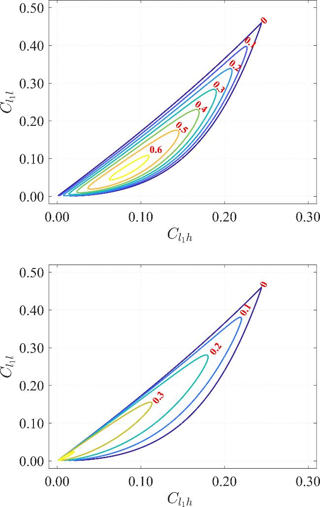
Figure 3. Variations of (a) work ${ \mathcal W }$ and (b) efficiency η with ${{ \mathcal C }}_{{l}_{1}{\rm{h}}}$ and ${{ \mathcal C }}_{{l}_{1}{\rm{l}}}$ in isoline maps. The parameters are Δ = 0.0, Ω = 5.0 and other common parameters are the same as figure 2. |
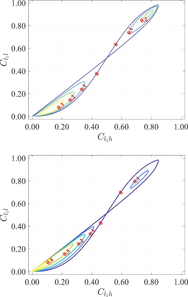
Figure 4. Variations of (a) work ${ \mathcal W }$ and (b) efficiency η with ${{ \mathcal C }}_{{l}_{1}{\rm{h}}}$ and ${{ \mathcal C }}_{{l}_{1}{\rm{l}}}$ in isoline maps. The parameters are Δ = 0.0, Ω = 25.0 and other common parameters are the same as figure 2. |
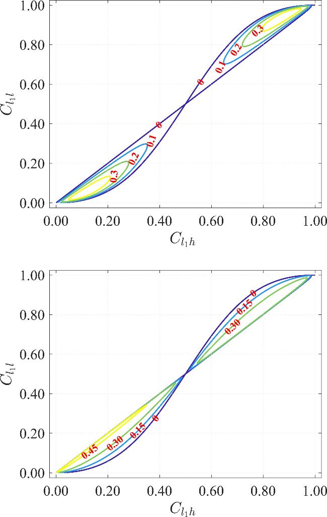
Figure 5. Variations of (a) work ${ \mathcal W }$ and (b) efficiency η with ${{ \mathcal C }}_{{l}_{1}{\rm{h}}}$ and ${{ \mathcal C }}_{{l}_{1}{\rm{l}}}$ in isoline maps. The parameters are Δ = 0.07D1Ω = 50.0 and other common parameters are the same as figure 2. |
The isolines of the work ${ \mathcal W }$ and the efficiency η are loops. These indicate that work ${ \mathcal W }$ and efficiency η no longer change monotonically with ${{ \mathcal C }}_{{l}_{1}{\rm{h}}}$ and ${{ \mathcal C }}_{{l}_{1}{\rm{l}}}$. In the regime of weak dipole coupling constants Ω, the resulting loop structures exhibit in narrower coherence domains, as illustrated in figure 3. Conversely, under strong dipole coupling conditions, these loop lines achieved - appearing either in narrower coherence domains or extending into broader spaces of ${{ \mathcal C }}_{{l}_{1}{\rm{h}}}$ and ${{ \mathcal C }}_{{l}_{1}{\rm{l}}}$, with comparative manifestations provided in figures 4 and 5, respectively. The loop lines become larger ones as the dipole-dipole coupling constant Ω increases. The acceptable range of ${{ \mathcal C }}_{{l}_{1}{\rm{h}}}$ and ${{ \mathcal C }}_{{l}_{1}{\rm{l}}}$ is ${{ \mathcal C }}_{{l}_{1}{\rm{h}}}\gt {{ \mathcal C }}_{{l}_{1}{\rm{l}}}$ or ${{ \mathcal C }}_{{l}_{1}{\rm{h}}}\lt {{ \mathcal C }}_{{l}_{1}{\rm{l}}}$ and varies with different constant Ω values. Conversely, the maximum work and efficiency increases as the dipole-dipole coupling constant Ω increases at a given temperature of the bath. There exists a maximum value work (or efficiency) ${{ \mathcal W }}_{\max }\left({\eta }_{\max }\right)$ when the quantum coherences ${{ \mathcal C }}_{{l}_{1}{\rm{h}}}$ and ${{ \mathcal C }}_{{l}_{1}{\rm{l}}}$ attain certain values. It is noteworthy that the interatomic coupling strength Ω not merely affects the shape of the work and the efficiency but ultimately governs its quantitative magnitude.
b) Non-identical Atoms, i.e. Δ ≠ 0.
Based on equations (20 ) and (21 ), we can obtain ${{ \mathcal G }}_{{\rm{h}}}$ and ${{ \mathcal G }}_{{\rm{l}}}$, as follows
$\begin{eqnarray}\begin{array}{rcl}{{ \mathcal G }}_{{\rm{h}}} & = & {\beta }_{{\rm{h}}}^{-1}\,\rm{arccosh}\,\left[\frac{{\rm{\Lambda }}}{{{ \mathcal C }}_{{l}_{1}{\rm{h}}}}\sinh \left({\beta }_{{\rm{h}}}\sqrt{{{\rm{\Delta }}}^{2}+{{\rm{\Omega }}}^{2}}\right)\right.\\ & & \left.-\cosh \left({\beta }_{{\rm{h}}}\sqrt{{{\rm{\Delta }}}^{2}+{{\rm{\Omega }}}^{2}}\right)\Space{0ex}{2.5ex}{0ex}\right],\end{array}\end{eqnarray}$
$\begin{eqnarray}\begin{array}{rcl}{{ \mathcal G }}_{{\rm{l}}} & = & {\beta }_{{\rm{l}}}^{-1}\,\rm{arccosh}\,\left[\frac{{\rm{\Lambda }}}{{{ \mathcal C }}_{{l}_{1}{\rm{l}}}}\sinh \left({\beta }_{{\rm{l}}}\sqrt{{{\rm{\Delta }}}^{2}+{{\rm{\Omega }}}^{2}}\right)\right.\\ & & \left.-\cosh \left({\beta }_{{\rm{l}}}\sqrt{{{\rm{\Delta }}}^{2}+{{\rm{\Omega }}}^{2}}\right)\Space{0ex}{2.5ex}{0ex}\right].\end{array}\end{eqnarray}$
Then all the thermodynamical quantities can be arranged as
$\begin{eqnarray}\begin{array}{l}{{ \mathcal Q }}_{{\rm{h}}}=\frac{2}{{{ \mathcal Z }}_{{\rm{l}}}}\left[\sqrt{{{\rm{\Delta }}}^{2}+{{\rm{\Omega }}}^{2}}\sinh \left({\beta }_{{\rm{l}}}\sqrt{{{\rm{\Delta }}}^{2}+{{\rm{\Omega }}}^{2}}\right)+{{ \mathcal G }}_{{\rm{h}}}\sinh \left({\beta }_{{\rm{l}}}{{ \mathcal G }}_{{\rm{l}}}\right)\right]\\ -\frac{2}{{{ \mathcal Z }}_{{\rm{h}}}}\left[\sqrt{{{\rm{\Delta }}}^{2}+{{\rm{\Omega }}}^{2}}\sinh \left({\beta }_{{\rm{h}}}\sqrt{{{\rm{\Delta }}}^{2}+{{\rm{\Omega }}}^{2}}\right)+{{ \mathcal G }}_{{\rm{h}}}\sinh \left({\beta }_{{\rm{h}}}{{ \mathcal G }}_{{\rm{h}}}\right)\right],\end{array}\end{eqnarray}$
and $\begin{eqnarray}\begin{array}{rcl}{{ \mathcal Q }}_{{\rm{l}}} & = & \frac{2}{{{ \mathcal Z }}_{{\rm{h}}}}\left[\sqrt{{{\rm{\Delta }}}^{2}+{{\rm{\Omega }}}^{2}}\sinh \left({\beta }_{{\rm{h}}}\sqrt{{{\rm{\Delta }}}^{2}+{{\rm{\Omega }}}^{2}}\right)+{{ \mathcal G }}_{{\rm{l}}}\sinh \left({\beta }_{{\rm{h}}}{{ \mathcal G }}_{{\rm{h}}}\right)\right]\\ & & -\frac{2}{{{ \mathcal Z }}_{{\rm{l}}}}\left[\sqrt{{{\rm{\Delta }}}^{2}+{{\rm{\Omega }}}^{2}}\sinh \left({\beta }_{{\rm{l}}}\sqrt{{{\rm{\Delta }}}^{2}+{{\rm{\Omega }}}^{2}}\right)+{{ \mathcal G }}_{{\rm{l}}}\sinh \left({\beta }_{{\rm{l}}}{{ \mathcal G }}_{{\rm{l}}}\right)\right].\end{array}\end{eqnarray}$
According to equations (41 ) and (42 ), the expressions of the work and the efficiency can be written as
$\begin{eqnarray}{ \mathcal W }=2\left({{ \mathcal G }}_{{\rm{h}}}-{{ \mathcal G }}_{{\rm{l}}}\right)\left(\frac{\sinh \left({\beta }_{{\rm{l}}}{{ \mathcal G }}_{{\rm{l}}}\right)}{{{ \mathcal Z }}_{{\rm{l}}}}-\frac{\sinh \left({\beta }_{{\rm{h}}}{{ \mathcal G }}_{{\rm{h}}}\right)}{{{ \mathcal Z }}_{{\rm{h}}}}\right),\end{eqnarray}$
and $\begin{eqnarray}\eta =\frac{1-{{ \mathcal G }}_{{\rm{l}}}/{{ \mathcal G }}_{{\rm{h}}}}{1+\frac{{{ \mathcal Z }}_{{\rm{h}}}\sinh \left({\beta }_{{\rm{l}}}\sqrt{{{\rm{\Delta }}}^{2}+{{\rm{\Omega }}}^{2}}\right)-{{ \mathcal Z }}_{{\rm{l}}}\sinh \left({\beta }_{{\rm{h}}}\sqrt{{{\rm{\Delta }}}^{2}+{{\rm{\Omega }}}^{2}}\right)}{{{ \mathcal Z }}_{{\rm{h}}}\sinh \left({\beta }_{{\rm{l}}}{{ \mathcal G }}_{{\rm{l}}}\right)-{{ \mathcal Z }}_{{\rm{l}}}\sinh \left({\beta }_{{\rm{h}}}{{ \mathcal G }}_{{\rm{h}}}\right)}\frac{\sqrt{{{\rm{\Delta }}}^{2}+{{\rm{\Omega }}}^{2}}}{{{ \mathcal G }}_{{\rm{h}}}}}.\end{eqnarray}$
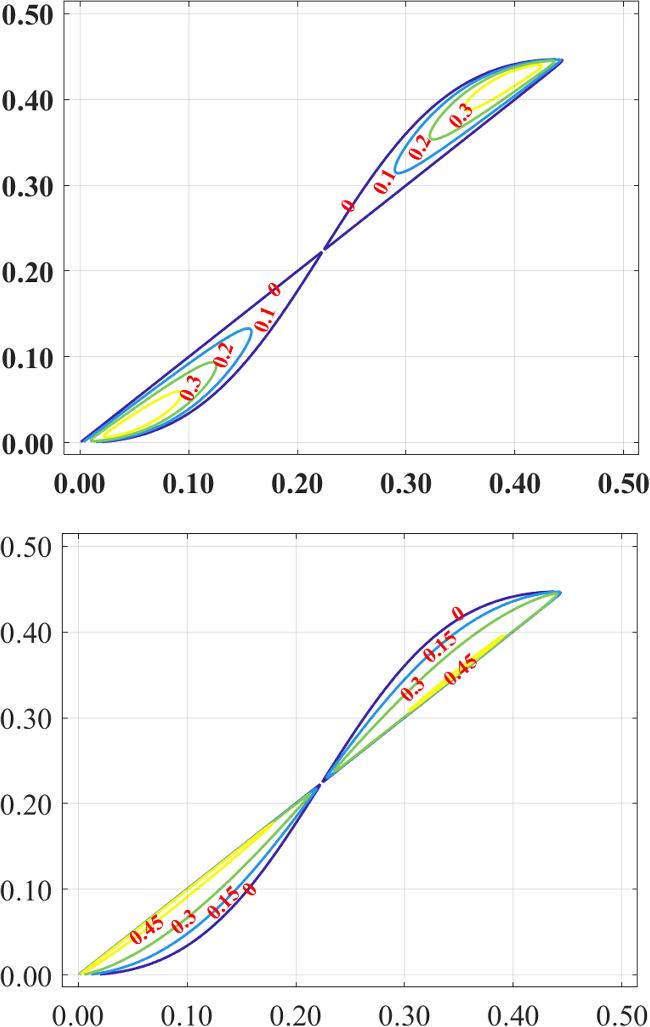
Based on equations (39 ), (40 ), (43 ) and (44 ), we can study the effects of quantum coherence on the basic thermodynamical quantities. The derivation of an analytical expression of the correlations among positive work, efficiency, and quantum coherence within the working substance constitutes a formidable theoretical challenge. To address this complexity, we resort to numerical simulations by adjusting the frequency detuning parameter (Δ) and analyze the interrelationships between these fundamental quantities, as shown in figures 6–8. By numerical calculation we can plot the isoline maps of the variation of the work and the efficiency with quantum coherence $\left({{ \mathcal C }}_{{l}_{1}{\rm{h}}},{{ \mathcal C }}_{{l}_{1}{\rm{l}}}\right)$ at three different frequency detuning Δ values for a pair of atoms, we assume the following parameters: Ω = 25.0, ${{ \mathcal T }}_{{\rm{h}}}=10.0$, ${{ \mathcal T }}_{{\rm{l}}}=5.0$ and kB = 1, as shown in figures 6–8.
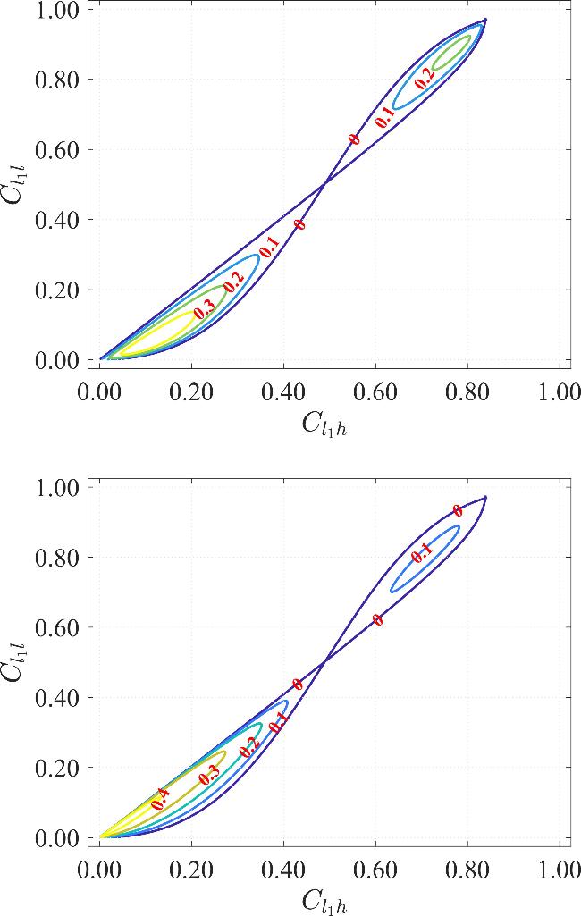
Figure 6. Variations of (a) work ${ \mathcal W }$ and (b) efficiency η with ${{ \mathcal C }}_{{l}_{1}{\rm{h}}}$ and ${{ \mathcal C }}_{{l}_{1}{\rm{l}}}$ in isoline maps. The parameters are Δ = 5.0, Ω = 25.0 and other common parameters are the same as figure 2. |
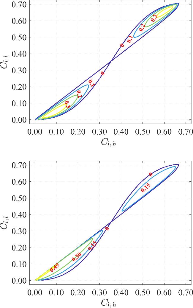
Figure 7. Variations of (a) work ${ \mathcal W }$ and (b) efficiency η with ${{ \mathcal C }}_{{l}_{1}{\rm{h}}}$ and ${{ \mathcal C }}_{{l}_{1}{\rm{l}}}$ in isoline maps. The parameters are Δ = 25.0, Ω = 25.0 and other common parameters are the same as figure 2. |
Figure 8. Variations of (a) work ${ \mathcal W }$ and (b) efficiency η with ${{ \mathcal C }}_{{l}_{1}{\rm{h}}}$ and ${{ \mathcal C }}_{{l}_{1}{\rm{l}}}$ in isoline maps. The parameters are Δ = 50.0, Ω = 25.0 and other common parameters are the same as figure 2. |
The loop lines become smaller ones as frequency detuning increases. Frequency detuning affects not only the shape of the efficiency but also its value. As shown in figures 6–8, the loop lines of work ${ \mathcal W }$ and efficiency η become smaller ones as the frequency detuning Δ increases. Thus, the frequency detuning Δ not only affects the shape of the work and the efficiency but also affects its value. This phenomenon can be elucidated through figure 2, which demonstrates that negative quantum coherence manifests when the frequency detuning exceeds a critical threshold. Furthermore, our analysis reveals that the maximum work (efficiency) ${{ \mathcal W }}_{\max }\left({\eta }_{\max }\right)$ exhibits an increasing trend with the increase of the frequency detuning Δ under conditions of quantum coherence ${{ \mathcal C }}_{{l}_{1}{\rm{h}}}\gt {{ \mathcal C }}_{{l}_{1}{\rm{l}}}$, whereas it demonstrates a decreasing tendency when the frequency detuning Δ is increased in the case of quantum coherence ${{ \mathcal C }}_{{l}_{1}{\rm{h}}}\lt {{ \mathcal C }}_{{l}_{1}{\rm{l}}}$. It is noteworthy that the maximum efficiency ${\eta }_{\max }$ demonstrates variability across differing frequency detuning. Moreover, we find that the Carnot efficiency ${\eta }_{{\rm{C}}}=1-{{ \mathcal T }}_{{\rm{l}}}/{{ \mathcal T }}_{{\rm{h}}}=0.5$ is not achievable in figures 3–8.
6. Relations between local and global efficiency
Each atom of two coupled two-level atoms in the subsystem can be assigned a local effective temperature, corresponding to its local thermal state or the reduced density matrix. This holds true regardless of the state of the total system. Particularly, in stages 1 and 3 of the QOE cycle, from equation (15 ), we get the local effective temperatures as
$\begin{eqnarray}\begin{array}{rcl}{{ \mathcal T }}_{{\rm{A}}\left({\rm{B}}\right),{\rm{h}}}^{{\rm{eff}}} & = & \hslash {\omega }_{{\rm{A}}\left({\rm{B}}\right)}\\ & & \times {\left[{k}_{{\rm{B}}}\mathrm{ln}\left(\frac{1}{{p}_{1{\rm{h}}}+\frac{1+{\rm{\Gamma }}}{2}{p}_{2{\rm{h}}}+\frac{1-{\rm{\Gamma }}}{2}{p}_{3{\rm{h}}}}-1\right)\right]}^{-1},\end{array}\end{eqnarray}$
and $\begin{eqnarray}{{ \mathcal T }}_{{\rm{A}}\left({\rm{B}}\right),{\rm{l}}}^{{\rm{eff}}}=\hslash {\omega }_{{\rm{A}}\left({\rm{B}}\right)}{\left[{k}_{{\rm{B}}}\mathrm{ln}\left(\frac{1}{{p}_{1{\rm{l}}}+\frac{1+{\rm{\Gamma }}}{2}{p}_{2{\rm{l}}}+\frac{1-{\rm{\Gamma }}}{2}{p}_{3{\rm{l}}}}-1\right)\right]}^{-1}.\end{eqnarray}$
The key observation is that in the presence of interactions, the local effective temperatures exhibit deviations from their corresponding bath temperatures: ${{ \mathcal T }}_{{\rm{A}}\left({\rm{B}}\right),{\rm{h}}}^{{\rm{eff}}}\ne {{ \mathcal T }}_{{\rm{h}}}$ and ${{ \mathcal T }}_{{\rm{A}}\left({\rm{B}}\right),{\rm{l}}}^{{\rm{eff}}}\ne {{ \mathcal T }}_{{\rm{l}}}$. In the quantum adiabatic processes, the energy spectrum of the system evolves while the occupation probabilities within the local two atoms remain invariant. Consequently, two coupled two-level atoms are subjected to quantum adiabatic evolution. Based on current analysis, it is evident that the cycle of the subsystem clearly constitutes a QOE. The (local) efficiency (in the absence of the interaction) is given by
$\begin{eqnarray}{\eta }_{0}=1-{{ \mathcal G }}_{{\rm{l}}}/{{ \mathcal G }}_{{\rm{h}}}.\end{eqnarray}$
It is interesting to know how much maximum efficiency is possible for a given set of parameters. In the case of ${{ \mathcal G }}_{{\rm{h}}}\gt {{ \mathcal G }}_{{\rm{l}}}$, under the positive work condition (PWC), we must have
$\begin{eqnarray}{p}_{1{\rm{h}}}-{p}_{4{\rm{h}}}-{p}_{1{\rm{l}}}+{p}_{4{\rm{l}}}=2\frac{{{\rm{e}}}^{2{\beta }_{{\rm{l}}}{{ \mathcal G }}_{{\rm{l}}}}-{{\rm{e}}}^{2{\beta }_{{\rm{h}}}{{ \mathcal G }}_{{\rm{h}}}}}{\left(1+{{\rm{e}}}^{2{\beta }_{{\rm{h}}}{{ \mathcal G }}_{{\rm{h}}}}\right)\left(1+{{\rm{e}}}^{2{\beta }_{{\rm{l}}}{{ \mathcal G }}_{{\rm{l}}}}\right)}\gt 0.\end{eqnarray}$
Then, we can obtain the additional condition
$\begin{eqnarray}{{ \mathcal G }}_{{\rm{l}}}/{{ \mathcal T }}_{{\rm{l}}}\gt {{ \mathcal G }}_{{\rm{h}}}/{{ \mathcal T }}_{{\rm{h}}}.\end{eqnarray}$
Based on equation (49 ), we take parameter $\sqrt{{{\rm{\Delta }}}^{2}+{{\rm{\Omega }}}^{2}}$ to satisfy ${ \mathcal G }-\sqrt{{{\rm{\Delta }}}^{2}+{{\rm{\Omega }}}^{2}}\gt 0$, so that ${ \mathcal G }$ is the first excited state, we get
$\begin{eqnarray}\frac{{{ \mathcal G }}_{{\rm{h}}}-\sqrt{{{\rm{\Delta }}}^{2}+{{\rm{\Omega }}}^{2}}}{{{ \mathcal T }}_{{\rm{h}}}}\lt \frac{{{ \mathcal G }}_{{\rm{l}}}-\sqrt{{{\rm{\Delta }}}^{2}+{{\rm{\Omega }}}^{2}}}{{{ \mathcal T }}_{{\rm{l}}}}.\end{eqnarray}$
Since, ${{ \mathcal G }}_{{\rm{h}}}-\sqrt{{{\rm{\Delta }}}^{2}+{{\rm{\Omega }}}^{2}}\gt 0\quad {{ \mathcal G }}_{{\rm{l}}}-\sqrt{{{\rm{\Delta }}}^{2}+{{\rm{\Omega }}}^{2}}\gt 0$ and ${{ \mathcal T }}_{{\rm{h}}}\gt {{ \mathcal T }}_{{\rm{l}}}$, From equation (50 ), We have an upper bound for the QOE efficiency 51 ) constitutes an upper bound to the efficiency of two coupled two-level atomic Otto engine which is tighter than Carnot efficiency.
$\begin{eqnarray}{\eta }_{{\rm{up}}}={\eta }_{{\rm{O}}}{\left(1-\sqrt{{{\rm{\Delta }}}^{2}+{{\rm{\Omega }}}^{2}}/{{ \mathcal G }}_{{\rm{h}}}\right)}^{-1}\lt {\eta }_{{\rm{C}}}=1-{{ \mathcal T }}_{{\rm{l}}}/{{ \mathcal T }}_{{\rm{h}}},\end{eqnarray}$
where ${\eta }_{{\rm{O}}}=1-{{ \mathcal G }}_{{\rm{l}}}/{{ \mathcal G }}_{{\rm{h}}}$ is the classical Otto engine (COE) efficiency (in the absence of the interaction). Equation (Finally, the (global) efficiency of the QOE with two baths at identical temperatures $\left({\beta }_{{\rm{h}}}={\beta }_{{\rm{l}}}={\beta }_{{\rm{s}}}\right)$, equations (30 ), (38 ), and (44 ) can be compactly formulated as follows:
$\begin{eqnarray}{\eta }_{{\rm{\Delta }}}=\frac{1-{{ \mathcal G }}_{{\rm{l}}}/{{ \mathcal G }}_{{\rm{h}}}}{1-\frac{{\rm{\Delta }}}{{{ \mathcal G }}_{{\rm{h}}}}\frac{2\sinh \left({\beta }_{{\rm{s}}}{\rm{\Delta }}\right)\sinh \left[{\beta }_{{\rm{s}}}\left({{ \mathcal G }}_{{\rm{h}}}+{{ \mathcal G }}_{{\rm{l}}}\right)/2\right]}{2\cosh \left[{\beta }_{{\rm{s}}}\left({{ \mathcal G }}_{{\rm{h}}}-{{ \mathcal G }}_{{\rm{l}}}\right)/2\right]+\cosh \left[{\beta }_{{\rm{s}}}{{\rm{\Xi }}}_{+{\rm{\Delta }}}\right]+\cosh \left[{\beta }_{{\rm{s}}}{{\rm{\Xi }}}_{-{\rm{\Delta }}}\right]}},\end{eqnarray}$
$\begin{eqnarray}{\eta }_{{\rm{\Omega }}}=\frac{1-{{ \mathcal G }}_{{\rm{l}}}/{{ \mathcal G }}_{{\rm{h}}}}{1-\frac{{\rm{\Omega }}}{{{ \mathcal G }}_{{\rm{h}}}}\frac{2\sinh \left({\beta }_{{\rm{s}}}{\rm{\Omega }}\right)\sinh \left[{\beta }_{{\rm{s}}}\left({{ \mathcal G }}_{{\rm{h}}}+{{ \mathcal G }}_{{\rm{l}}}\right)/2\right]}{2\cosh \left[{\beta }_{{\rm{s}}}\left({{ \mathcal G }}_{{\rm{h}}}-{{ \mathcal G }}_{{\rm{l}}}\right)/2\right]+\cosh \left[{\beta }_{{\rm{s}}}{{\rm{\Xi }}}_{+{\rm{\Omega }}}\right]+\cosh \left[{\beta }_{{\rm{s}}}{{\rm{\Xi }}}_{-{\rm{\Omega }}}\right]}},\end{eqnarray}$
and $\begin{eqnarray}\eta =\frac{1-{{ \mathcal G }}_{{\rm{l}}}/{{ \mathcal G }}_{{\rm{h}}}}{1-\frac{\sqrt{{{\rm{\Delta }}}^{2}+{{\rm{\Omega }}}^{2}}}{{{ \mathcal G }}_{{\rm{h}}}}\frac{2\sinh \left({\beta }_{{\rm{s}}}\sqrt{{{\rm{\Delta }}}^{2}+{{\rm{\Omega }}}^{2}}\right)\sinh \left[{\beta }_{{\rm{s}}}\left({{ \mathcal G }}_{{\rm{h}}}+{{ \mathcal G }}_{{\rm{l}}}\right)/2\right]}{2\cosh \left[{\beta }_{{\rm{s}}}\left({{ \mathcal G }}_{{\rm{h}}}-{{ \mathcal G }}_{{\rm{l}}}\right)/2\right]+\cosh \left[{\beta }_{{\rm{s}}}{{\rm{\Xi }}}_{+}\right]+\cosh \left[{\beta }_{S}{{\rm{\Xi }}}_{-}\right]}},\end{eqnarray}$
where Ξ± = $\sqrt{{{\rm{\Delta }}}^{2}+{{\rm{\Omega }}}^{2}}$ $\pm \,\left({{ \mathcal G }}_{{\rm{h}}}-{{ \mathcal G }}_{{\rm{l}}}\right)/2$, Ξ±Δ = ${\rm{\Delta }}\,\pm \left({{ \mathcal G }}_{{\rm{h}}}-{{ \mathcal G }}_{{\rm{l}}}\right)/2$, Ξ±Ω = ${\rm{\Omega }}\pm \left({{ \mathcal G }}_{{\rm{h}}}-{{ \mathcal G }}_{{\rm{l}}}\right)/2$.The interaction between the system and the reservoirs gives rise to entropy production arising from quantum coherence. This entropy can be quantitatively characterized and is directly related to the efficiency of the heat engine. The fundamental principles underlying the second law of thermodynamics remain inviolate nevertheless, the QOE exhibits distinct characteristics that are unattainable in classical engines.
7. Conclusions
In summary, we have studied the quantum Otto engine cycle with a pair of two-level atoms working system. Based on the thermal coherence and the first law of thermodynamics in a quantum system, expressions for the heat transferred, the work and the efficiency have been obtained. It is found that the work and efficiency does not change monotonically with quantum coherence $\left({{ \mathcal C }}_{{l}_{1}{\rm{h}}},{{ \mathcal C }}_{{l}_{1}{\rm{l}}}\right)$. The coupling constant Ω and the frequency detuning not only affect the shape of the efficiency but also affect its value. The acceptable range of ${{ \mathcal C }}_{{l}_{1}{\rm{h}}}$ and ${{ \mathcal C }}_{{l}_{1}{\rm{l}}}$ varies with different coupling constant and frequency detuning values. Our study reveals that quantum coherence can be enhanced by increasing the coupling constant or reducing the frequency detuning, accompanied by a corresponding reduction in the operational ranges for positive work and thermodynamic efficiency. When the coupling constant is large enough, the maximum efficiency approaches the Carnot efficiency. It is expected that our work will be of some help in the process of realizing quantum Otto engine.