


Introduction
The existence of matter in nature and the laboratory has various forms: for example, water can be liquid, gaseous or solid, and their transitions are one of the central issues in condensed matter physics and statistical physics [1, 2]. According to Ehrenfest’s classification, phase transitions can be categorized according to the behavior of the derivatives of energy (or free energy at finite temperature) with respect to temperature or other thermodynamic variables at the transition point. If the first derivative of energy is discontinuous, then the phase transition is of the first order; otherwise, the phase transition is of the second order if the second derivative is discontinuous, assuming its first derivative is continuous, and the rest may be deduced by analogy. Second-order phase transitions or above are usually called continuous phase transitions, which can be described phenomenologically by order parameter and associated broken symmetry [3, 4]. Furthermore, a complete theoretical description has been obtained using renormalization groups [5, 6]. In particular, the concepts of universality class and critical scaling characterized by critical exponents [1, 5, 6] can be used to classify the phase transitions, irrespective of the type of matter.
In contrast to the situation of the continuous phase transition, the investigations into first-order phase transitions are far from clear. The reason for this is that, except for the latent heat realized early on by the van der Waals equation of state [7], the first-order phase transition lacks typical features characterized by its critical behavior, just like the order parameters and associated broken symmetries in the continuous phase transitions. As a result, the concept, like the order parameter, can only be used cautiously in the study of first-order phase transitions [8, 9]. However, a robust observation is that there is a metastable equilibrium region in the vicinity of the first-order transition point, where at least two or more possible metastable states compete with each other for a long time before the first-order phase transition takes place. The formation of a new phase is usually initiated when the nucleation of the new phase commences, which has been popularly observed in liquid–gas or liquid–solid phase transitions [1].
Here, we present an example to exhibit a first-order quantum phase transition (QPT) in one of the simplest many-body systems, namely, the transverse Ising model (TIM), under an additional longitudinal field. It is well known that the ground state of the TIM experiences a second-order QPT from the paramagnetic phase in the weak interaction regime to the ferromagnetic phase in the strong interaction regime [10–12]. This phase transition is characterized by the degeneracy of the ground state and first excited-state energy levels, as shown in figure 1(a). Furthermore, this QPT is accompanied by spontaneous Z2 symmetry breaking, leading to the spins of the collective alignment of spins along either the up or down direction. Due to its simplicity and well-understood critical behavior, the TIM has served as a paradigmatic model for studying continuous QPTs. In our previous work [13], we have used the pattern picture to dissect the process of this QPT, in which the pattern characterizing the ferromagnetic order becomes dominant over the others in a smooth way as the interaction strength J increases. As a result, the occurrence of the QPT is not so dramatic.
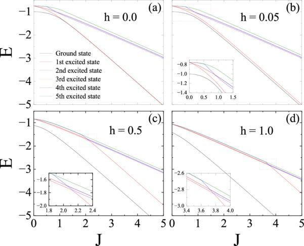
Figure 1. The energy spectra of the ground state and first five excited states of the 1D transverse Ising model in the absence (a) and presence (b)–(d) of longitudinal fields. The insets in (b), (c) and (d) show enlarged views of the crossovers of excited states. The system size is taken as L = 8. |
The introduction of a weak longitudinal field profoundly alters this behavior by explicitly breaking the Z2 symmetry and rendering the system non-integrable. In this case, the QPT in the ground state is suppressed. The ferromagnetic order persists for all interaction strengths, i.e. ⟨σz⟩ ≠ 0, and the ground state and first excited state no longer become degenerate but instead remain separated by a finite small energy gap, as shown in figure 1(b). As the longitudinal field increases, for example, h = 0.5 and h = 1.0, we find that interesting physics is involved in the excited states, where the first excited state at large J rapidly approaches the second excited state in which a spin is flipped, and they go across to lead to a first-order QPT, as shown in figures 1(c) and (d). To our knowledge, this phenomenon has not been previously reported in the literature.
In this work, we employ the pattern picture method to systematically investigate the characteristics of the first-order QPT. In contrast to the standard TIM, where the transition is governed by a single dominant pattern [13], the longitudinal field induces competition between multiple distinct patterns during the first-order transition. Furthermore, we perform a comparative analysis between the first-order QPT in the first excited state in the presence of a longitudinal field and a continuous QPT in the ground state in the absence of a longitudinal field, on an equal level.
Model and method
The TIM Hamiltonian with a longitudinal field reads 1 ) is rewritten as 4 ) can be diagonalized to obtain eigenvalues and corresponding eigenfunctions {λn, un}(n = 1, 2, ⋯ , 3L). By using {λn, un}, equation (4 ) is reformulated as
$\begin{eqnarray}{\hat{H}}^{{\prime} }=-{J}^{{\prime} }\displaystyle \sum _{j,\delta }{\hat{\sigma }}_{j}^{z}{\hat{\sigma }}_{j+1}^{z}-{h}^{{\prime} }\displaystyle \sum _{j}{\hat{\sigma }}_{j}^{z}-g\displaystyle \sum _{j}{\hat{\sigma }}_{j}^{x},\end{eqnarray}$
where ${J}^{{\prime} }$ is the Ising interaction between two spins denoted by the Pauli matrix $\hat{\sigma }$ located at site j and its nearest neighbors j + δ. Here, ${h}^{{\prime} }$ and g are the longitudinal and transverse fields, respectively. All these parameters are non-negative, and thus the interaction is ferromagnetic. For convenience, we take the transverse field g as units of energy. This is different from the conventional notations in the literature [10], but we find that it is more convenient to use the present notations to discuss the first-order excited-state QPT. Thus, equation ( $\begin{eqnarray}{\hat{H}}^{{\prime} }=\frac{g}{2}\hat{H},\ \hat{H}=\displaystyle \sum _{j}{\hat{H}}_{j},\end{eqnarray}$
$\begin{eqnarray}{\hat{H}}_{j}=-2{\hat{\sigma }}_{j}^{x}-2h{\hat{\sigma }}_{j}^{z}-J\displaystyle \sum _{\delta }\left({\hat{\sigma }}_{j}^{z}{\hat{\sigma }}_{j+\delta }^{z}+{\hat{\sigma }}_{j+\delta }^{z}{\hat{\sigma }}_{j}^{z}\right),\end{eqnarray}$
where $J={J}^{{\prime} }/g$ and $h={h}^{{\prime} }/g$. For simplicity, we limit ourselves to the one-dimensional (1D) case; therefore, δ equals 1. For a chain with size L under periodic boundary conditions (PBC, i.e. ${\hat{\sigma }}_{L+1}^{z}={\hat{\sigma }}_{1}^{z}$), $\hat{H}$ can be reformulated as a 3L × 3L matrix in a spin operator space as follows $\begin{eqnarray}\begin{array}{rcl}\hat{H} & = & \left(\begin{array}{cccccccccc}{\hat{\sigma }}_{1}^{x} & -{\rm{i}}{\hat{\sigma }}_{1}^{y} & {\hat{\sigma }}_{1}^{z} & {\hat{\sigma }}_{2}^{x} & -{\rm{i}}{\hat{\sigma }}_{2}^{y} & {\hat{\sigma }}_{2}^{z} & \cdots \, & {\hat{\sigma }}_{L}^{x} & -{\rm{i}}{\hat{\sigma }}_{L}^{y} & {\hat{\sigma }}_{L}^{z}\end{array}\right)\\ & & \times \left(\begin{array}{cccccccccc}0 & h & 0 & 0 & 0 & 0 & \cdots \, & 0 & 0 & 0\\ h & 0 & -1 & 0 & 0 & 0 & \cdots \, & 0 & 0 & 0\\ 0 & -1 & 0 & 0 & 0 & -J & \cdots \, & 0 & 0 & -J\\ 0 & 0 & 0 & 0 & h & 0 & \cdots \, & 0 & 0 & 0\\ 0 & 0 & 0 & h & 0 & -1 & \cdots \, & 0 & 0 & 0\\ 0 & 0 & -J & 0 & -1 & 0 & \cdots \, & 0 & 0 & 0\\ \vdots & \vdots & \vdots & \vdots & \vdots & \vdots & \ddots & \vdots & \vdots & \vdots \\ 0 & 0 & 0 & 0 & 0 & 0 & \cdots \, & 0 & h & 0\\ 0 & 0 & 0 & 0 & 0 & 0 & \cdots \, & h & 0 & -1\\ 0 & 0 & -J & 0 & 0 & 0 & \cdots \, & 0 & -1 & 0\end{array}\right)\\ & & \times {\left(\begin{array}{cccccccccc}{\hat{\sigma }}_{1}^{x} & i{\hat{\sigma }}_{1}^{y} & {\hat{\sigma }}_{1}^{z} & {\hat{\sigma }}_{2}^{x} & i{\hat{\sigma }}_{2}^{y} & {\hat{\sigma }}_{2}^{z} & \cdots \, & {\hat{\sigma }}_{L}^{x} & i{\hat{\sigma }}_{L}^{y} & {\hat{\sigma }}_{L}^{z}\end{array}\right)}^{{\rm{T}}},\end{array}\end{eqnarray}$
where the identities ${\hat{\sigma }}^{x}{\hat{\sigma }}^{y}={\rm{i}}{\hat{\sigma }}^{z}$ and ${\hat{\sigma }}^{y}{\hat{\sigma }}^{z}={\rm{i}}{\hat{\sigma }}^{x}$ have been used for each site j. The superscript T denotes the transpose of the operator vector. The matrix in equation ( $\begin{eqnarray}\hat{H}=\displaystyle \sum _{n=1}^{3L}{\lambda }_{n}{\hat{A}}_{n}^{\dagger }{\hat{A}}_{n},\end{eqnarray}$
where the obtained operator ${\hat{A}}_{n}$ is composed of single-body operators $\begin{eqnarray}{\hat{A}}_{n}=\displaystyle \underset{j=1}{\overset{L}{\oplus }}\left[{u}_{n,3j-2}{\hat{\sigma }}_{j}^{x}+{u}_{n,3j-1}({\rm{i}}{\hat{\sigma }}_{j}^{y})+{u}_{n,3j}{\hat{\sigma }}_{j}^{z}\right].\end{eqnarray}$
The symbol $\oplus $ denotes Kronecker sum. We refer to the operators ${\hat{A}}_{n}$ as patterns, each characterized by its corresponding eigenvalue λn. Obviously, there are three spin components $({\sigma }_{j}^{x},{\rm{i}}{\hat{\sigma }}_{j}^{y},{\hat{\sigma }}_{j}^{z})$ for each lattice site j, where ${\hat{\sigma }}_{j}^{z}$ represents spin-up/down and the other two represent the flip of spins.Characters of patterns
To explicitly show the pattern configurations, we extract the signs (positive or negative) of the eigenvectors (un,3j−2, un,3j−1, un,3j) at each lattice site j. For a system with lattice size L, each pattern exhibits L pairs of signs, as shown in figure 2, which represent the relative phase of the three operators {σx, iσy, σz}. In the absence of a longitudinal field (h = 0), the operator ${\hat{A}}_{n}$ lacks the ${\sigma }_{j}^{x}$ term, resulting in 2L distinct patterns that can be categorized into two groups based on their eigenvalues: one with λn < 0 and the other with λn > 0. Further details regarding the pattern formulation in the standard TIM can be found in [13].
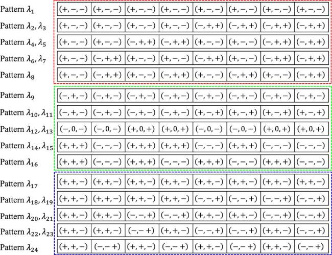
Figure 2. The patterns and their relative phases marked by the single-body operators, equation ( |
When a longitudinal field is applied (h ≠ 0), the operator ${\hat{A}}_{n}$ incorporates all three spin operators, leading to 3L patterns. figures 2 and 3 display the patterns and their corresponding eigenvalue dependencies on the interaction strength J. According to the behavior of the eigenvalues shown in figure 3, all the patterns can be divided into three groups, which are degenerate for each group at J = 0, and the degeneracy is partly lifted as J increases. The patterns show several characteristic features: (i) except for patterns λ12,13 with zero pattern eigenvalues, the patterns with negative eigenvalues have opposite signs for the coefficients of ${\hat{\sigma }}_{j}^{x}$ and ${\rm{i}}{\hat{\sigma }}_{j}^{y}$, namely, they are out-of-phase; (ii) oppositely, they are in-phase for the patterns with positive eigenvalues; (iii) the distinguishing features between different patterns in each group are the signs of the coefficients of ${\hat{\sigma }}_{j}^{z}$ and their orders, which correspond to different domains or kinks contained in the patterns; (iv) patterns λ1, λ9 and λ17 are especially important since their eigenvalues are the lowest in their own groups, and there is a common characteristic, namely, the coefficients of ${\hat{\sigma }}_{j}^{z}$ are in-phase, which are possible candidates of metastable states; (v) in each group, the patterns with two domains or kinks, such as patterns λ2,3, patterns λ10,11 and patterns λ18,19, are also potential candidates of metastable states, which are important to the excited-state QPT that we are studying.
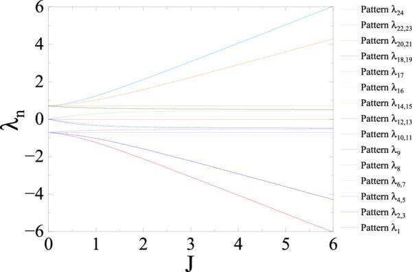
Figure 3. The eigenvalues λn of patterns as functions of J. The system size and the longitudinal field are taken as L = 8 and h = 1.0, respectively. The eigenvalues of the patterns satisfy λn = − λ3L−n+1. |
The above observations are independent of the system size [13]. While larger system sizes produce more patterns with increased domain/kink complexity, the fundamental features described above remain unchanged. This explains why the essential physics of QPT can be effectively captured by the pattern picture, even in small systems, as demonstrated in our analysis.
First-order excited-state QPT
After clarifying the obtained pattern picture, we solve the Hamiltonian denoted by equation (5 ) by inserting it into the complete basis $| \{{\sigma }_{j}^{z}\}\rangle (j=1,2,\cdots \,,L)$ with ${\hat{\sigma }}_{j}^{z}| \{{\sigma }_{j}^{z}\}\rangle ={\pm }_{j}(\uparrow ,\downarrow )| \{{\sigma }_{j}^{z}\}\rangle $. One can easily write the single-body operator ${\hat{A}}_{n}$ in matrix form, 5 ) can be solved by diagonalizing the matrix
$\begin{eqnarray}{\left[{\hat{A}}_{n}\right]}_{\{{\sigma }_{j}^{z}\},\{{\sigma }_{j}^{z}\}^{\prime} }=\langle \{{\sigma }_{j}^{z}\}| {\hat{A}}_{n}| \{{\sigma }_{j}^{z}\}^{\prime} \rangle .\end{eqnarray}$
Then equation ( $\begin{eqnarray}\begin{array}{l}\langle \{{\sigma }_{j}^{z}\}| \hat{H}| \{{\sigma }_{j}^{z}\}^{\prime} \rangle =\langle \{{\sigma }_{j}^{z}\}| \displaystyle \sum _{n=1}^{3L}{\lambda }_{n}{\hat{A}}_{n}^{\dagger }{\hat{A}}_{n}| \{{\sigma }_{j}^{z}\}^{\prime} \rangle \\ =\displaystyle \sum _{n=1}^{3L}{\lambda }_{n}\langle \{{\sigma }_{j}^{z}\}| {\hat{A}}_{n}^{\dagger }{\hat{A}}_{n}| \{{\sigma }_{j}^{z}\}^{\prime} \rangle \\ =\displaystyle \sum _{n=1}^{3L}{\lambda }_{n}\displaystyle \sum _{{\{{\sigma }_{j}^{z}\}}^{{\prime\prime} }}{\left[{\hat{A}}_{n}^{\dagger }\right]}_{\{{\sigma }_{j}^{z}\},{\{{\sigma }_{j}^{z}\}}^{{\prime\prime} }}{\left[{\hat{A}}_{n}\right]}_{{\{{\sigma }_{j}^{z}\}}^{{\prime\prime} },\{{\sigma }_{j}^{z}\}^{\prime} }.\end{array}\end{eqnarray}$
After obtaining the wavefunctions $\Psi$i (i = 0, 1,⋯, corresponding to the ground state, the first excited state and so on, respectively), we project the wavefunction onto different patterns to calculate the contributions of different patterns to the interested physical quantities. For example, the energy contributions of different patterns are calculated using the formula $\begin{eqnarray}{E}_{{\lambda }_{n}}={\lambda }_{n}\langle {{\rm{\Psi }}}_{i}| {\hat{A}}_{n}^{\dagger }{\hat{A}}_{n}| {{\rm{\Psi }}}_{i}\rangle ,(n=1,2,\cdots \,,3L).\end{eqnarray}$
Here, we define another physical quantity, namely, the patterns’ occupancy $\begin{eqnarray}{O}_{{\lambda }_{n}}=\langle {{\rm{\Psi }}}_{i}| {\hat{A}}_{n}^{\dagger }{\hat{A}}_{n}| {{\rm{\Psi }}}_{i}\rangle ,(n=1,2,\cdots \,,3L).\end{eqnarray}$
figures 4(a1) and (b1) present the energies of the ground and first excited states as functions of the interaction J for h = 1.0, respectively, as shown by thick black solid lines. The results of numerical exact diagonalization (ED) (circles) are also presented for comparison, which confirms the validity of the pattern formulation. As shown in figures 1(b)–(d), the ground state is always dominant over the first excited state and, in this case, the system is always ferromagnetic. Therefore, there is no QPT occurrence in the ground state, as also seen from the smooth first-order derivative and second-order derivative shown in figure 4(a2).
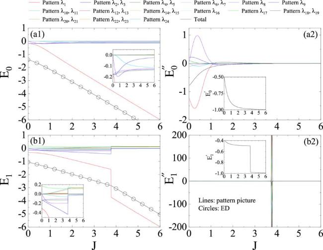
Figure 4. (a1) and (b1) The ground state and first excited-state energies (thick black lines) and their corresponding pattern components (colored lines) as functions of J. Circles represent the results of numerical ED. The insets in (a1) and (b1) denote the enlarged views. (a2) and (b2) The second-order derivatives of the energy components of patterns. The insets in (a2) and (b2) denote the first-order derivatives of the total energy. Here, h = 1.0 is taken and the system size is L = 8. |
Turning to the first excited state, the situation changes dramatically. An obvious discontinuity of the first excited-state energy is seen near J ≈ 4.0, as shown in figure 4(b1). This first-order QPT is more apparent when checking the contributions of pattern components to the first excited-state energy, especially that of pattern λ1. Enlarged views of the other components are shown in the inset of figure 4(b1). The energy of pattern λ1 has a sudden drop at J ≈ 4.0, even lower than the energy of the first excited state. At the same time, other patterns, such as λ2,3, λ9 and λ17, also exhibit dramatic changes. They indeed form metastable states, which have a local minimum. In particular, patterns λ2,3 even directly compete with pattern λ1; they have comparable energy contributions to the first excited state at small J. Another important observation is the response of the patterns with positive eigenvalues, which are excited by the first-order QPT, and their suppressions are slow as the interaction strength increases. Moreover, this phase transition is also seen from the sharp first-order and second-order derivatives in figure 4(b2).
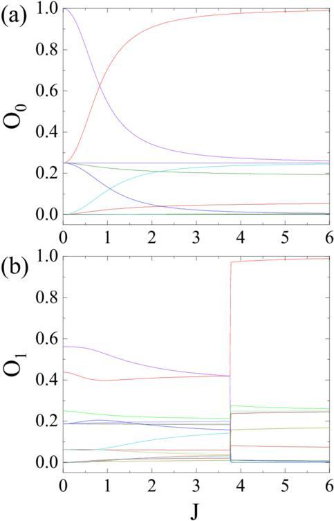
The above observations can be further confirmed by examining the pattern occupancies, calculated using equation (10 ), as shown in figure 5 for h = 1.0. For the ground state shown in figure 5(a), it is seen that the pattern occupancies vary smoothly with increasing J, much more smoothly than in the ground state at h = 0.0 (where a second-order QPT exists [13]), causing the QPT to smear out. Additionally, in the small J region, pattern λ9 surpasses pattern λ1, which differs from when h = 0.0, while in the large J region, pattern λ1 dominates over others, consistent with the standard TIM. As seen in figure 2, both pattern λ1 and pattern λ9 represent ferromagnetic order with their signs of σz being in-phase. Therefore, the interaction-induced ferromagnetic order is predominantly manifested in pattern λ1, whereas the external longitudinal field-induced ferromagnetic order is correspondingly reflected in pattern λ9.
Figure 5. (a) The patterns’ occupancies of the ground state, and (b) the first excited state under a longitudinal field h = 1.0 as functions of J. The legend is the same as figure 4. |
The situation is quite different in the first excited state, as shown in figure 5(b). Below the transition point, pattern λ1 and pattern λ9 contribute nearly equally, reflecting a competitive interplay between these patterns. When the transition point is reached, pattern λ1 surpasses pattern λ9, dominating the strong interaction regime. This competition, along with the abrupt transition, is characteristic of metastable state formation—a hallmark of first-order transitions. Additionally, patterns λ2,3, patterns λ4,5, patterns λ6,7, pattern λ8 and pattern λ17 also exhibit reduced but non-negligible contributions. These observations are consistent with the energy distribution trends.
A comparative analysis of pattern occupancy reveals key distinctions between QPT types: in the second-order QPTs, only one pattern, namely, pattern λ1, flavoring the ferromagnetic phase, is always dominant over others [13]. However, in the first-order QPTs, there are at least two competitive patterns, such as patterns λ1, λ2,3 and λ9, which form metastable states. This is the main difference between these two kinds of QPTs. Furthermore, in the TIM with an applied longitudinal field, while both the ground state and the first excited state are ultimately governed by pattern λ1 at large interaction strength J, the difference is the occupancies of the other patterns due to quantum fluctuations. In the ground state, the other occupancies mainly distribute near pattern λ9 and, in the first excited state, these occupancies mainly locate near pattern λ17. Thus these two cases are complementary, which may be useful in quantum annealing [14–17] and involves dynamics of the model we are studying. This is obviously beyond the scope of the present work and is left for the future.
Based on the above discussion, the pattern picture provides a different approach for probing phase transitions, which differs fundamentally from conventional methods. This approach involves a decomposition of the Hamiltonian into distinct components, each of which exhibits characteristic responses to variations in system parameters. By analyzing these responses, the pattern picture provides an effective characterization of phase transitions. Besides the TIM investigated here, this method can be extended to frustrated systems, such as the 1D axial next-nearest-neighbor Ising model in a transverse field [18], the spin-1/2 J1-J2 antiferromagnetic Heisenberg model on the square lattice [19] and the Shastry–Sutherland model [20].
Summary and discussion
The well-known second-order QPT in the TIM in the ground state is smeared out once a longitudinal field is applied. Instead, a first-order QPT is found in the first excited state. We provide the pattern picture obtained by two successive diagonalizations to study these two QPTs on an equal level. While the second-order QPT in the absence of a longitudinal field has been studied in detail in [13], here we mainly focus on the case with a finite longitudinal field.
After the energy contributions of different patterns to the ground and first excited states have been clearly analyzed, how to smear out the second-order QPT and how to form the first-order QPT are further identified. In particular, the comparison between the patterns’ occupancies of the first excited state in the presence of the longitudinal field and those of the ground state in the absence of the longitudinal field characterizes the different processes of the first-order and second-order QPTs: in the second-order QPT, the patterns flavoring the ferromagnetic phase are dominant over others and the phase transition is somehow not so dramatic. By contrast, in the first-order case that we study here, there are at least two competitive patterns and, as a result, the first-order QPT is so dramatic.
The first excited-state QPT obtained in the present work could be tested by current quantum simulation platforms [21], ranging from trapped ions [22, 23], quantum superconducting circuits [16, 24] to optical lattices [25], and so on. The non-integrability of the system in the presence of a longitudinal field further enriches the phase transition physics involved in such a paradigmatic model.