Welcome to visit Communications in Theoretical Physics,
Quantum Physics and Quantum Information

Separability criteria and entanglement witnesses from mutually unbiased equiangular tight frames

  • Alexey E Rastegin
Expand
  • Irkutsk State University, K. Marx St. 1, Irkutsk 664003, Russia

Received date: 2025-05-29

  Revised date: 2025-09-20

  Accepted date: 2025-09-24

  Online published: 2025-10-23

Copyright

© 2025 Institute of Theoretical Physics CAS, Chinese Physical Society and IOP Publishing. All rights, including for text and data mining, AI training, and similar technologies, are reserved.
This article is available under the terms of the IOP-Standard License.

Abstract

Methods of quantum information processing often appear in terms of specially selected states. For example, mutually unbiased bases (MUBs) and symmetric informationally complete measurements are widely applied. Finite frames have found use in many areas including quantum information. Due to its specific inner structure, a single equiangular tight frame (ETF) allows one to formulate criteria to detect non-classical correlations. This study aims to approach entanglement detection with the use of mutually unbiased ETFs. Such frames are an interesting generalization of widely recognized MUBs. It still uses rank-one operators, but the number of outcomes can exceed the dimensionality. Several approaches are considered including separability criteria and entanglement witnesses. Separability criteria for multipartite systems are finally obtained.

Cite this article

Alexey E Rastegin . Separability criteria and entanglement witnesses from mutually unbiased equiangular tight frames[J]. Communications in Theoretical Physics, 2026 , 78(2) : 025104 . DOI: 10.1088/1572-9494/ae0abb

1. Introduction

Quantum entanglement is especially important from the conceptual viewpoint as well as for emerging technologies of quantum information processing [1, 2]. The existence of such correlations in quantum systems was independently emphasized in the Schrödinger ‘cat paradox’ paper [3] and the Einstein–Podolsky–Rosen paper [4]. Further development of these questions was notably pushed up by Bohm’s reformulation of the Einstein–Podolsky–Rosen thought experiment (see section 16 of chapter 22 of reference [5]). Quantum entanglement is at the core of parallel processing on a quantum computer [6]. The factorization algorithm of Shor [7] and the search algorithm of Grover [8, 9] were first examples of the quantum speed-up. Although the power of quantum computing is certainly limited [10], this concept seems to actualize in recent future. There are physical platforms recognized as a potential way to construct quantum processors [1114]. Thus, possible ways to characterize quantum entanglement are required to develop new technologies. For 2 ⨂ 2 and 2 ⨂ 3 systems, the question is resolved by the Peres–Horodecki criterion [1518]. Entanglement in other systems is more complicated to examine. Methods based on the moments of the partially transposed density matrix were proposed for the certification and benchmarking of medium-size quantum devices [19].
Quantum measurements typically appeared as a final step to complete the protocol of interest. Specially built sets of quantum states are a requisite for many purposes including entanglement detection. Mutually unbiased bases (MUBs) [20] are the well-know example of discrete structures in Hilbert spaces [21]. They were first considered by Schwinger [22] and later applied to quantum state determination [23, 24]. Reference [25] provided a constructive proof of the existence of MUBs. This approach was used to study quantum key distribution [26] and cloning machines [27]. Projective two-designs are another example of vectors with useful properties [28, 29]. Recently, equiangular tight frames (ETFs) have been shown to be useful in quantum information [3032]. Such frames of finite-dimensional vectors were originally studied without applications [33, 34]. A symmetric informationally complete measurement [35] can be interpreted as an ETF with the maximal number of kets allowed for the given dimensionality. Mutually unbiased ETFs were proposed rather as a way to produce new frames from existing ones [36]. Extending MUBs, such frames deserve further development in various topics including quantum information [37, 38]. Other ways to fit the concept of mutual unbiasedness were accomplished [3941].
This study aims to examine mutually unbiased ETFs as a tool for entanglement detection. Several ways to obtain needed criteria will be addressed. The so-called correlation measure was originally proposed for MUBs [42]. It was later adopted for a symmetric informationally complete measurement [43], mutually unbiased measurements [44] and a single ETF [30]. It will be realized with measurements assigned to a mutually-unbiased-ETF. Entanglement witnesses can be built with the use of positive maps obtained from MUBs [45] and vectors of an ETF [32]. Both these constructions are particular cases of the maps described in this paper. Criteria to test multipartite entanglements are also of interest. Reference [32] showed the use of a single ETF to check fully separable tripartite states. It will be extended in the following two respects. First, we reformulate the approach with mutually unbiased ETFs. Second, the results for fully separable multipartite states will be presented. This paper is organized as follows. Section 2 reviews the preliminary material. Section 3 presents the main results. Section 4 concludes the paper. Appendix derives auxiliary statements.

2. Preliminaries

In this section, we discuss the required material and fix the notation. First, the basic facts about quantum states and measurements will be given. Also, we recall the concept of separable quantum states. Second, mutually unbiased ETFs will be considered.

2.1. Quantum states and measurements

Let ${ \mathcal L }({{ \mathcal H }}_{d})$ be the space of linear operators on d-dimensional Hilbert space ${{ \mathcal H }}_{d}$. By ${{ \mathcal L }}_{+}({{ \mathcal H }}_{d})$ and ${{ \mathcal L }}_{sa}({{ \mathcal H }}_{d})$, we respectively mean the set of positive semi-definite operators and the real space of Hermitian ones. In the given computational basis, operators of interest are represented by rectangular matrices with complex entries. Matrix norms are widely used to characterize matrices quantitatively [46]. In the following, we will use the Frobenius norm. For the given m × n matrix A = [[aij]], its Frobenius norm is calculated as
$\begin{eqnarray}\parallel {\boldsymbol{A}}{\parallel }_{2}={\left(\displaystyle \sum _{i=1}^{m}\displaystyle \sum _{j=1}^{n}| {a}_{ij}{| }^{2}\right)}^{1/2}.\end{eqnarray}$
The square of this norm is equal to the trace of AA. The right-hand side of (1) can be extended to the case of entries with three or more indices.
The states of a system with Hilbert space ${{ \mathcal H }}_{d}$ are described by density matrices, i.e. by positive semi-definite operators on ${{ \mathcal H }}_{d}$ with unit trace. In general, quantum measurements are described by positive operator-valued measures (POVMs) [47]. Each POVM is a set of operators ${{\boldsymbol{E}}}_{j}\in {{ \mathcal L }}_{+}({{ \mathcal H }}_{d})$ that obey the completeness relation
$\begin{eqnarray}\displaystyle \sum _{j=1}^{n}{{\boldsymbol{E}}}_{j}={{\mathbb{1}}}_{d},\end{eqnarray}$
where n is the number of measurement outcomes and ${{\mathbb{1}}}_{d}$ is the identity operator on ${{ \mathcal H }}_{d}$. It is principally important that n can exceed d. Informationally complete measurements allow us to estimate the expectation value of an arbitrary operator by just averaging functions of the experimental outcomes [48]. For the pre-measurement state ρ, the probability of jth outcome reads as [47]
$\begin{eqnarray}{p}_{j}({ \mathcal E };{\boldsymbol{\rho }})={\rm{tr}}({{\boldsymbol{E}}}_{j}{\boldsymbol{\rho }}).\end{eqnarray}$
The index of coincidence is defined as
$\begin{eqnarray}I({ \mathcal E };{\boldsymbol{\rho }})=\displaystyle \sum _{j=1}^{n}{p}_{j}{({ \mathcal E };{\boldsymbol{\rho }})}^{2}.\end{eqnarray}$
It will be used to characterize probability distributions quantitatively. Due to estimates on the index (equation (4)), useful inequalities for information entropies can be obtained [49]. In more detail, characterization of probability distribution is discussed in chapter 2 of the book [50].
Let us recall basic notions related to separable states of a bipartite system. By A and B, we denote subsystems of a bipartite system with Hilbert space ${{ \mathcal H }}_{AB}={{ \mathcal H }}_{A}\otimes {{ \mathcal H }}_{B}$. Product states are described by density matrices of the form ρA ⨂ ρB [50]. A bipartite mixed state is called separable, when its density matrix ${\tilde{{\boldsymbol{\rho }}}}_{AB}$ can be represented as a convex combination of product states [51, 52]. That is, there exists a representation of the form
$\begin{eqnarray}{\tilde{{\boldsymbol{\rho }}}}_{AB}={\sum }_{\ell }{w}^{(\ell )}\,{{\boldsymbol{\rho }}}_{A}^{(\ell )}\otimes {{\boldsymbol{\rho }}}_{B}^{(\ell )},\end{eqnarray}$
where w() ≥ 0 and ∑w() = 1. The case of multipartite entanglement is more complicated to analyze. Fully separable tripartite states are represented by density matrices of the form
$\begin{eqnarray}{\tilde{{\boldsymbol{\rho }}}}_{ABC}={\sum }_{{\ell }}{w}^{({\ell })}\,{{\boldsymbol{\rho }}}_{A}^{({\ell })}\otimes {{\boldsymbol{\rho }}}_{B}^{({\ell })}\otimes {{\boldsymbol{\rho }}}_{C}^{({\ell })}.\end{eqnarray}$
ETFs were shown to be useful to detect entanglement in bipartite [30] and tripartite systems [32]. Similarly to equation (6), fully separable K-partite states are expressed as
$\begin{eqnarray}{\tilde{{\boldsymbol{\rho }}}}_{{A}_{1}\cdots {A}_{K}}={\sum }_{\ell }{w}^{(\ell )}\,{{\boldsymbol{\rho }}}_{{A}_{1}}^{(\ell )}\otimes {{\boldsymbol{\rho }}}_{{A}_{2}}^{(\ell )}\otimes \cdots \otimes {{\boldsymbol{\rho }}}_{{A}_{K}}^{(\ell )}.\end{eqnarray}$
It will be shown that mutually unbiased ETFs give a tool to detect entanglement in multipartite systems.

2.2. Mutually unbiased equiangular tight frames

Finite tight frames are a rapidly growing area with many applications including those in quantum theory (see, e.g. chapter 14 of [53]). A set $\left\{| {\phi }_{j}\rangle \right\}$ of nd unit vectors of ${{ \mathcal H }}_{d}$ is a tight frame, when [39]
$\begin{eqnarray}\displaystyle \sum _{j=1}^{n}| {\phi }_{j}\rangle \langle {\phi }_{j}| =\frac{n}{d}\,{{\mathbb{1}}}_{d}.\end{eqnarray}$
If it is holds that
$\begin{eqnarray}{\left|\langle {\phi }_{i}| {\phi }_{j}\rangle \right|}^{2}=c,\end{eqnarray}$
for all i ≠ j, then we deal with an ETF. It can be shown that nd2,
$\begin{eqnarray}c=\frac{n-d}{(n-1)d},\qquad 1-c=\frac{n(d-1)}{(n-1)d}.\end{eqnarray}$
An ETF of n = d2 vectors, if it exists in ${{ \mathcal H }}_{d}$, leads to a symmetric informationally complete measurement (SIC-POVM) ${ \mathcal N }=\left\{{{\boldsymbol{N}}}_{j}\right\}$ with elements
$\begin{eqnarray}{{\boldsymbol{N}}}_{j}=\frac{1}{d}\,| {\phi }_{j}\rangle \langle {\phi }_{j}| .\end{eqnarray}$
The existence of such sets for all d was conjectured by Zauner [21]. Reference [35] considered SIC-POVMs in more detail.
The notion of a mutually-unbiased-ETF was proposed [36]. Suppose that 1 ≤ M and 1 ≤ dn. A sequence $\left\{| {\phi }_{\mu j}\rangle \right\}$ of unit vectors with μ = 1, …, M and j = 1, …, n is a mutually-unbiased-ETF if [36]
$\begin{eqnarray}{\left|\langle {\phi }_{\mu i}| {\phi }_{\nu j}\rangle \right|}^{2}=\left\{\begin{array}{ll}c,\quad & \mu =\nu \,\,\rm{and}\,\,i\ne j,\\ {d}^{-1},\quad & \mu \ne \nu ,\end{array}\right.\end{eqnarray}$
where c is given by equation (10). That is, this mutually-unbiased-ETF consists of M usual ETFs.
The special case with n = d and c = 0 reduces to a set of M MUBs. Such bases give an example of complementary observables in finite dimensions [54]. The BB84 scheme of quantum cryptography [55] actually deals with two MUBs. The authors of the work [40] proposed mutually unbiased measurements. Such measurements are similar to MUBs, but rank-one elements are not used. On the other hand, rank-one POVMs are often of primary meaning [56]. Several ETFs with the fixed overlap between vectors of different frames can be treated as another capable extension of MUBs. It still uses rank-one POVMs, but the number of outcomes can exceed the dimensionality. The latter is valuable in quantum information, for example, in unambiguous state discrimination [57] and probabilistic quantum cloning [58]. The task to distinguish quantum states by local operations and classical communication is very important in information processing. Its character changes essentially when entangled states are dealt with [59]. This problem was also shown to be closely related with MUBs [59]. It would be interesting to examine distinguishanbility of entangled states with mutually unbiased ETFs.
Now, we exemplify a mutually-unbiased-ETF with c ≠ 0. It deals with a ququart in dimension four. The vectors of mutually unbiased ETFs arise as columns of the matrices ϒ, Δϒ, Δ2ϒ, where [36]
$\begin{eqnarray}\begin{array}{r}{\boldsymbol{\Upsilon }}=\frac{1}{2}\left(\begin{array}{ccccc}1 & {\omega }^{3} & {\omega }^{6} & {\omega }^{9} & {\omega }^{12}\\ 1 & {\omega }^{6} & {\omega }^{12} & {\omega }^{3} & {\omega }^{9}\\ 1 & {\omega }^{9} & {\omega }^{3} & {\omega }^{12} & {\omega }^{6}\\ 1 & {\omega }^{12} & {\omega }^{9} & {\omega }^{6} & {\omega }^{3}\end{array}\right),\end{array}\end{eqnarray}$
$\begin{eqnarray}\begin{array}{l}{\boldsymbol{\Delta }}=\left(\begin{array}{cccc}\omega & 0 & 0 & 0\\ 0 & {\omega }^{2} & 0 & 0\\ 0 & 0 & {\omega }^{8} & 0\\ 0 & 0 & 0 & {\omega }^{4}\end{array}\right),\end{array}\end{eqnarray}$
and $\omega =\exp ({\rm{i}}2\pi /15)$. In this example, we have d = 4, n = 5 and M = 3.
Each of M ETFs induces a non-orthogonal resolution ${{ \mathcal F }}^{(\mu )}={\left\{{{\boldsymbol{F}}}_{i}^{(\mu )}\right\}}_{i=1}^{n}$ of the identity with rank-one elements
$\begin{eqnarray}{{\boldsymbol{F}}}_{i}^{(\mu )}=\frac{d}{n}\,| {\phi }_{\mu i}\rangle \langle {\phi }_{\mu i}| ,\end{eqnarray}$
since
$\begin{eqnarray}\frac{d}{n}\,\displaystyle \sum _{i=1}^{n}| {\phi }_{\mu i}\rangle \langle {\phi }_{\mu i}| ={{\mathbb{1}}}_{d}.\end{eqnarray}$
For each μ, the probability of ith outcome reads as
$\begin{eqnarray}{p}_{i}({{ \mathcal F }}^{(\mu )};{\boldsymbol{\rho }})=\frac{d}{n}\,\langle {\phi }_{\mu i}| {\boldsymbol{\rho }}| {\phi }_{\mu i}\rangle .\end{eqnarray}$
Putting these probabilities in (4) gives the μth index of coincidence $I({{ \mathcal F }}^{(\mu )};{\boldsymbol{\rho }})$. To a mutually-unbiased-ETF, we also assign a single POVM ${ \mathcal Q }=\{{{\boldsymbol{Q}}}_{\mu i}\}$ with rank-one elements
$\begin{eqnarray}{{\boldsymbol{Q}}}_{\mu i}=\frac{d}{Mn}\,| {\phi }_{\mu i}\rangle \langle {\phi }_{\mu i}| .\end{eqnarray}$
The probability of μith outcome then appears as
$\begin{eqnarray}{p}_{\mu i}({ \mathcal Q };{\boldsymbol{\rho }})=\frac{d}{Mn}\,\langle {\phi }_{\mu i}| {\boldsymbol{\rho }}| {\phi }_{\mu i}\rangle .\end{eqnarray}$
It follows from equations (17) and (19) that
$\begin{eqnarray}I({ \mathcal Q };{\boldsymbol{\rho }})=\frac{1}{{M}^{2}}\,\displaystyle \sum _{\mu =1}^{M}I({{ \mathcal F }}^{(\mu )};{\boldsymbol{\rho }}).\end{eqnarray}$
Here, the total index of coincidence $I({ \mathcal Q };{\boldsymbol{\rho }})$ is obtained from equation (4) by substituting the probabilities (equation (19)). The formula (20) links two different interpretations of measurement data. It was shown in the appendix of the work [37] that
$\begin{eqnarray}\displaystyle \sum _{\mu =1}^{M}I({{ \mathcal F }}^{(\mu )};{\boldsymbol{\rho }})\leqslant \frac{(1-c)\left[{d}^{2}\,{\rm{tr}}({{\boldsymbol{\rho }}}^{2})-d\right]}{{n}^{2}}+\frac{M}{n}.\end{eqnarray}$
This result follows from the structural properties of a mutually-unbiased-ETF. For generalized ETFs, similar results for the indices of coincidence were obtained in the papers [41, 60].

3. Main results

This section will present new criteria to detect entanglement. The first way uses a generalization of the so-called correlation measure. This measure based on MUBs was originally proposed [42]. Another approach to the problem of entanglement detection was developed in the paper [18]. It deals with positive maps to obtain entanglement witnesses. Also, criteria for multipartite systems will be considered.

3.1. Correlation measures with mutually unbiased ETFs

It is known that entanglement detection can be realized with MUBs [42], MUMs [44] and a single ETF [30, 32]. To use a mutually-unbiased-ETF for entanglement detection, we extend the method considered in the works [42, 43]. Let us take a bipartite system of two d-dimensional subsystems. For each $| \varphi \rangle \in {{ \mathcal H }}_{d}$, we introduce ∣φ*⟩ as the ket with the conjugate components in the canonical basis. To the given mutually-unbiased-ETF, we assign M2 POVMs with elements
$\begin{eqnarray*}\frac{{d}^{2}}{{n}^{2}}\,| {\phi }_{\mu i}\rangle \langle {\phi }_{\mu i}| \otimes | {\phi }_{\nu j}^{* }\rangle \langle {\phi }_{\nu j}^{* }| .\end{eqnarray*}$
For a density matrix ${\tilde{{\boldsymbol{\rho }}}}_{AB}$ of the bipartite system, the (i, j)-probability reads as
$\begin{eqnarray}\frac{{d}^{2}}{{n}^{2}}\,\langle {\phi }_{\mu i}{\phi }_{\nu j}^{* }| {\tilde{{\boldsymbol{\rho }}}}_{AB}| {\phi }_{\mu i}{\phi }_{\nu j}^{* }\rangle .\end{eqnarray}$
Summing these probabilities over all μ = ν and i = j, we obtain the correlation measure
$\begin{eqnarray}G\left({\tilde{{\boldsymbol{\rho }}}}_{AB}\right)=\frac{{d}^{2}}{{n}^{2}}\,\displaystyle \sum _{\mu =1}^{M}\displaystyle \sum _{j=1}^{n}\langle {\phi }_{\mu j}{\phi }_{\mu j}^{* }| {\tilde{{\boldsymbol{\rho }}}}_{AB}| {\phi }_{\mu j}{\phi }_{\mu j}^{* }\rangle .\end{eqnarray}$
The following statement holds.

Let ${\tilde{{\boldsymbol{\rho }}}}_{AB}$ be a separable bipartite state on ${{ \mathcal H }}_{d}\otimes {{ \mathcal H }}_{d}$; then

$\begin{eqnarray}G\left({\tilde{{\boldsymbol{\rho }}}}_{AB}\right)\leqslant \frac{(1-c)({d}^{2}-d)}{{n}^{2}}+\frac{M}{n}.\end{eqnarray}$

For any product state ρA ⨂ ρB, the probability (equation (22)) is a product of two local probabilities. Using equation (21) and the Cauchy–Schwarz inequality, we obtain

$\begin{eqnarray}\begin{array}{rcl}G\left({{\boldsymbol{\rho }}}_{A}\displaystyle \otimes {{\boldsymbol{\rho }}}_{B}\right) & \leqslant & {\left(\frac{(1-c)\left[{d}^{2}\,{\rm{tr}}({{\boldsymbol{\rho }}}_{A}^{2})-d\right]}{{n}^{2}}+\frac{M}{n}\right)}^{1/2}\\ & & \times {\left(\frac{(1-c)\left[{d}^{2}\,{\rm{tr}}({{\boldsymbol{\rho }}}_{B}^{2})-d\right]}{{n}^{2}}+\frac{M}{n}\right)}^{1/2}.\end{array}\end{eqnarray}$
Combining the latter with ${\rm{tr}}({{\boldsymbol{\rho }}}_{A}^{2})\leqslant 1$ and ${\rm{tr}}({{\boldsymbol{\rho }}}_{B}^{2})\leqslant 1$ leads to the inequality
$\begin{eqnarray*}G\left({{\boldsymbol{\rho }}}_{A}\otimes {{\boldsymbol{\rho }}}_{B}\right)\leqslant \frac{(1-c)({d}^{2}-d)}{{n}^{2}}+\frac{M}{n}.\end{eqnarray*}$
Merging this formula with equation (5) completes the proof.  

The statement of proposition 1 gives a separability criterion with the use of mutually unbiased ETFs. Substituting n = d and c = 0 gives the case of M MUBs originally considered in the work [42]. Then we have
$\begin{eqnarray}G\left({\tilde{{\boldsymbol{\rho }}}}_{AB}\right)\leqslant 1+\frac{M-1}{d}.\end{eqnarray}$
For M = 1, the obtained equation (24) reduces to the already discussed case of a single ETF [30].
Using an orthonormal basis ${\left\{| {e}_{i}\rangle \right\}}_{i=1}^{d}$ in ${{ \mathcal H }}_{d}$, we write a maximally entangled state
$\begin{eqnarray*}| {{\rm{\Phi }}}_{+}\rangle =\frac{1}{\sqrt{d}}\,\displaystyle \sum _{i=1}^{d}| {e}_{i}\rangle \otimes | {e}_{i}\rangle .\end{eqnarray*}$
It is immediate to get $\langle {\phi }_{\mu j}{\phi }_{\mu j}^{* }| {{\rm{\Phi }}}_{+}\rangle =1/\sqrt{d}$, whence
$\begin{eqnarray}G\left(| {{\rm{\Phi }}}_{+}\rangle \langle {{\rm{\Phi }}}_{+}| \right)=\frac{Md}{n}.\end{eqnarray}$
To characterize a region of detectability, we divide the right-hand side of equation (24) by equation (27). The ratio is calculated as
$\begin{eqnarray}\frac{d-2+n/d}{M(n-1)}+\frac{M-1}{Md}\leqslant \frac{M+d-1}{Md},\end{eqnarray}$
whenever nd. The right-hand side of equation (28) corresponds to the case of M MUBs. When d is a prime power, there exist M = d + 1 MUBs and the right-hand side of equation (28) reduces to 2/(d + 1).

3.2. Entanglement witnesses via positive maps

The following result was proved [16, 18]. A bipartite quantum state ${\tilde{{\boldsymbol{\rho }}}}_{AB}$ is separable if and only if $({\rm{id}}\otimes {\rm{\Psi }})({\tilde{{\boldsymbol{\rho }}}}_{AB})\geqslant {\bf{0}}$ for every positive map ${\rm{\Psi }}:\,{ \mathcal L }({{ \mathcal H }}_{B})\to { \mathcal L }({{ \mathcal H }}_{A})$. Here, the identity map acts as id(ρA) = ρA. An operator $\tilde{{\boldsymbol{W}}}\in {{ \mathcal L }}_{sa}({{ \mathcal H }}_{A}\otimes {{ \mathcal H }}_{B})$ is an entanglement witness if it is not positive and
$\begin{eqnarray}\langle \varphi \otimes \varphi ^{\prime} | \tilde{{\boldsymbol{W}}}| \varphi \otimes \varphi ^{\prime} \rangle \geqslant 0,\end{eqnarray}$
for all $| \varphi \rangle \in {{ \mathcal H }}_{A}$ and $| \varphi ^{\prime} \rangle \in {{ \mathcal H }}_{B}$ [2, 61, 62]. Reference [63] discussed in general entanglement witnesses constructed from symmetric measurements. We aim to construct entanglement witnesses with a mutually-unbiased-ETF.
Let us consider a family of orthogonal n × n matrices R(μ) with real entries, and let each of these matrices leaves the vector ${(1,1,\ldots ,1)}^{{\mathsf{T}}}$ invariant. Then elements of each matrix satisfy the two conditions,
$\begin{eqnarray}\begin{array}{r}\displaystyle \sum _{i=1}^{n}{R}_{ij}^{(\mu )}=1,\end{array}\end{eqnarray}$
$\begin{eqnarray}\begin{array}{r}\displaystyle \sum _{i=1}^{n}{R}_{ij}^{(\mu )}{R}_{ik}^{(\mu )}={\delta }_{jk},\end{array}\end{eqnarray}$
where δjk is the Kronecker symbol. The special class of orthogonal matrices with the required properties is provided by permutations [45]. We define the following linear map,
$\begin{eqnarray}{\rm{\Psi }}({\boldsymbol{X}})={\rm{tr}}({\boldsymbol{X}}){{\boldsymbol{\rho }}}_{* }-\eta \displaystyle \sum _{\mu =1}^{M}\displaystyle \sum _{i,j=1}^{n}{R}_{ij}^{(\mu )}{\rm{tr}}\left(\bar{{\boldsymbol{X}}}{{\boldsymbol{F}}}_{j}^{(\mu )}\right){{\boldsymbol{F}}}_{i}^{(\mu )},\end{eqnarray}$
where ${{\boldsymbol{\rho }}}_{* }={{\mathbb{1}}}_{d}/d$ is the maximally mixed state, and $\bar{{\boldsymbol{X}}}={\boldsymbol{X}}-{\rm{tr}}({\boldsymbol{X}}){{\boldsymbol{\rho }}}_{* }$ for brevity. Also, the positive parameter η is defined as
$\begin{eqnarray}\eta =\frac{n(n-1)}{d{(d-1)}^{2}}.\end{eqnarray}$
It is shown in Appendix that the above map is positive and trace-preserving. An entanglement witness ${\tilde{{\boldsymbol{W}}}}_{{\rm{\Psi }}}\in {{ \mathcal L }}_{sa}({{ \mathcal H }}_{d}\otimes {{ \mathcal H }}_{d})$ assigned to a positive but not completely positive map (32) reads as
$\begin{eqnarray}{\tilde{{\boldsymbol{W}}}}_{{\rm{\Psi }}}=\displaystyle \sum _{i,j=1}^{d}| {e}_{i}\rangle \langle {e}_{j}| \otimes {\rm{\Psi }}\left(| {e}_{i}\rangle \langle {e}_{j}| \right),\end{eqnarray}$
where ${\left\{| {e}_{i}\rangle \right\}}_{i=1}^{d}$ is an orthonormal basis in ${{ \mathcal H }}_{d}$. This method was applied with a set of MUBs in the work [45] and for a single ETF in the work [32]. Thus, we have generalized these constructions to a set of M ETFs. It allows one to detect entanglement for bipartite systems.
The simplest choice for orthogonal matrices is the identity matrix of the corresponding size. When d + 1 MUBs exist in ${{ \mathcal H }}_{d}$, putting ${R}_{ij}^{(\mu )}={\delta }_{ij}$ for all μ = 1, …, d + 1 finally leads to the map [45]
$\begin{eqnarray}{\rm{\Psi }}^{\prime} ({\boldsymbol{X}})=\frac{{\rm{tr}}({\boldsymbol{X}}){{\mathbb{1}}}_{d}-{\boldsymbol{X}}}{d-1}.\end{eqnarray}$
Up to a factor, this positive map was used in the work [64] to derive an example of the reduction criterion. It should be emphasized that this example can be constructed with the use of an SIC-POVM. Using a single ETF in ${{ \mathcal H }}_{d}$ with n = d2 and the identity matrix as the orthogonal one, we get
$\begin{eqnarray}{{\rm{\Psi }}}^{{\prime\prime} }({\boldsymbol{X}})={\rm{tr}}({\boldsymbol{X}}){{\boldsymbol{\rho }}}_{* }-\frac{{d}^{2}+d}{d-1}\,\displaystyle \sum _{j=1}^{{d}^{2}}{\rm{tr}}\left(\bar{{\boldsymbol{X}}}{{\boldsymbol{N}}}_{j}\right){{\boldsymbol{N}}}_{j},\end{eqnarray}$
where the elements of an SIC-POVM read as equation (11). As is shown in Appendix, for all ${\boldsymbol{X}}\in { \mathcal L }({{ \mathcal H }}_{d})$ one has
$\begin{eqnarray}\displaystyle \sum _{j=1}^{{d}^{2}}{\rm{tr}}\left({\boldsymbol{X}}{{\boldsymbol{N}}}_{j}\right){{\boldsymbol{N}}}_{j}=\frac{{\rm{tr}}({\boldsymbol{X}}){{\mathbb{1}}}_{d}+{\boldsymbol{X}}}{{d}^{2}+d}.\end{eqnarray}$
Applying (36) to $\bar{{\boldsymbol{X}}}={\boldsymbol{X}}-{\rm{tr}}({\boldsymbol{X}}){{\boldsymbol{\rho }}}_{* }$ and combining the result with equation (37), we obtain
$\begin{eqnarray}\begin{array}{r}\begin{array}{rcl}{{\rm{\Psi }}}^{{\prime\prime} }({\boldsymbol{X}}) & = & {\rm{tr}}({\boldsymbol{X}}){{\boldsymbol{\rho }}}_{* }-\frac{{\boldsymbol{X}}-{\rm{tr}}({\boldsymbol{X}}){{\boldsymbol{\rho }}}_{* }}{d-1}\\ & = & \frac{{\rm{tr}}({\boldsymbol{X}}){{\mathbb{1}}}_{d}-{\boldsymbol{X}}}{d-1}.\end{array}\end{array}\end{eqnarray}$
It seems that this link of SIC-POVMs to positive maps was not yet discussed in the literature. If Zauner’s conjecture is true, the map (equation (38)) follows from equation (32) for all d. The right-hand side of equation (36) reduces to equation (35), thought was more complicated initially. It was obtained independently of the assumption that d + 1 MUBs exist in ${{ \mathcal H }}_{d}$.

3.3. Criteria for multipartite systems

The case of bipartite systems is only the first step in studies of multipartite entanglement. In recent literature, separability criteria for tripartite and multipartite systems have found use. We begin with the case of a tripartite system. Let ${\tilde{{\boldsymbol{\rho }}}}_{ABC}$ be a tripartite mixed state of the system with the Hilbert space ${{ \mathcal H }}_{d}\otimes {{ \mathcal H }}_{d}\otimes {{ \mathcal H }}_{d}$. To adopt a mutually-unbiased-ETF, we will use a single POVM with the elements (18). To the given state ${\tilde{{\boldsymbol{\rho }}}}_{ABC}$ and a POVM $\tilde{{ \mathcal E }}$ with the elements ${{\boldsymbol{E}}}_{i}\otimes {{\boldsymbol{E}}}_{j}^{{\prime} }\otimes {{\boldsymbol{E}}}_{k}^{{\prime\prime} }$, we assign the corresponding matrix ${\boldsymbol{\Lambda }}(\tilde{{ \mathcal E }};{\tilde{{\boldsymbol{\rho }}}}_{ABC})$ with entries
$\begin{eqnarray}{\rm{tr}}\left[({{\boldsymbol{E}}}_{i}\otimes {{\boldsymbol{E}}}_{j}^{{\prime} }\otimes {{\boldsymbol{E}}}_{k}^{{\prime\prime} }){\tilde{{\boldsymbol{\rho }}}}_{ABC}\right].\end{eqnarray}$
Then the following statement takes place.

Let ${\tilde{{\boldsymbol{\rho }}}}_{ABC}$ be a fully separable tripartite state on ${{ \mathcal H }}_{d}\otimes {{ \mathcal H }}_{d}\otimes {{ \mathcal H }}_{d}$; then

$\begin{eqnarray}{\parallel {\boldsymbol{\Lambda }}(\tilde{{ \mathcal Q }};{\tilde{{\boldsymbol{\rho }}}}_{ABC})\parallel }_{2}\leqslant \frac{1}{{M}^{3}}{\left(\frac{(1-c)({d}^{2}-d)}{{n}^{2}}+\frac{M}{n}\right)}^{3/2},\end{eqnarray}$
where $\tilde{{ \mathcal Q }}$ contains elements of the form Qλi ⨂ Qμj ⨂ Qνk assigned to a mutually-unbiased-ETF.

It will be sufficient to prove the claim for a product state ρA ⨂ ρB ⨂ ρC. Then the final result follows due to the triangle inequality. Immediate calculations show that

$\begin{eqnarray}\begin{array}{r}\begin{array}{l}{\parallel \Space{0ex}{0.25ex}{0ex}{\boldsymbol{\Lambda }}\,(\tilde{{ \mathcal Q }};{{\boldsymbol{\rho }}}_{A}\displaystyle \otimes {{\boldsymbol{\rho }}}_{B}\displaystyle \otimes {{\boldsymbol{\rho }}}_{C})\Space{0ex}{0.25ex}{0ex}\parallel }_{2}^{2}\\ =\displaystyle \sum _{\lambda ,\mu ,\nu ,=1}^{M}\displaystyle \sum _{i,j,k=1}^{n}{\left[{\rm{tr}}({{\boldsymbol{Q}}}_{\lambda i}{{\boldsymbol{\rho }}}_{A})\,{\rm{tr}}({{\boldsymbol{Q}}}_{\mu j}{{\boldsymbol{\rho }}}_{B})\,{\rm{tr}}({{\boldsymbol{Q}}}_{\nu k}{{\boldsymbol{\rho }}}_{C})\right]}^{2}\\ =\,I\,({ \mathcal Q };{{\boldsymbol{\rho }}}_{A})I({ \mathcal Q };{{\boldsymbol{\rho }}}_{B})I({ \mathcal Q };{{\boldsymbol{\rho }}}_{C})\\ \leqslant \,\frac{1}{{M}^{6}}{\left(\frac{(1-c)({d}^{2}-d)}{{n}^{2}}+\frac{M}{n}\right)}^{3}.\end{array}\end{array}\end{eqnarray}$
Here, the last step follows by combining equation (20) with equation (21). The obtained inequality (41) proves equation (40) for all states of the form ρA ⨂ ρB ⨂ ρC.  

For M = 1, the statement of proposition 2 reproduces the criterion reported in the paper [32]. It is natural to extend equation (40) to the case of multupartite systems. This extension is derived by an immediate reformulation of the above proof. We refrain from presenting the details here. In this way, we have arrived at a conclusion.

Let ${\tilde{{\boldsymbol{\rho }}}}_{{A}_{1}\cdots {A}_{K}}$ be a fully separable K-partite state on ${{ \mathcal H }}_{d}^{\,\otimes K}$; then

$\begin{eqnarray}{\parallel {\boldsymbol{\Lambda }}(\tilde{{ \mathcal Q }};{\tilde{{\boldsymbol{\rho }}}}_{{A}_{1}\cdots {A}_{K}})\parallel }_{2}\leqslant \frac{1}{{M}^{K}}{\left(\frac{(1-c)({d}^{2}-d)}{{n}^{2}}+\frac{M}{n}\right)}^{K/2},\end{eqnarray}$
where the POVM $\tilde{{ \mathcal Q }}$ contains elements of the form
$\begin{eqnarray}\displaystyle \underset{k=1}{\overset{K}{\otimes }}{{\boldsymbol{Q}}}_{{\mu }_{k}{j}_{k}},\end{eqnarray}$
assigned to a mutually-unbiased-ETF.

Of course, fully separable states are only one of several forms of separable states allowed in a multipartite system. Nevertheless, the statement of proposition 3 shows a utility of ETF-based measurements in studies of multipartite entanglement.

3.4. Examples

Let us consider concrete examples of the use of mutually unbiased ETFs to detect entanglement. Isotropic states are often used to test separability criteria. For q ∈ [0, 1], one considers the density matrix
$\begin{eqnarray}{\tilde{{\boldsymbol{\varrho }}}}_{{\rm{iso}}}=\frac{1-q}{{d}^{2}}\,{{\mathbb{1}}}_{d}\otimes {{\mathbb{1}}}_{d}+q\,| {{\rm{\Phi }}}_{+}\rangle \langle {{\rm{\Phi }}}_{+}| .\end{eqnarray}$
These states are entangled if and only if q > 1/(d + 1) [64]. It can be checked immediately that
$\begin{eqnarray*}G\left({\tilde{{\boldsymbol{\varrho }}}}_{{\rm{iso}}}\right)=\frac{M(qd+1-q)}{n}.\end{eqnarray*}$
Combining this with equation (24) shows that the violation occurs for
$\begin{eqnarray}q\gt \frac{d-1}{M(n-1)}.\end{eqnarray}$
For M = 1, this inequality was reported in the work [30]. The case of an SIC-POVM with n = d2 implies detectability for q > 1/(d + 1) [30]. For the case of M MUBs, the inequality (45) reads as q > 1/M as reported in the paper [42]. It becomes q > 1/(d + 1) when M = d + 1 MUBs exists in dimension d. Thus, we have obtained the least cases previously mentioned in the literature.
Further, we consider bipartite states on ${{ \mathcal H }}_{4}\otimes {{ \mathcal H }}_{4}$, which are of the form
$\begin{eqnarray}{\tilde{{\boldsymbol{\sigma }}}}_{AB}={a}_{1}{\tilde{{\boldsymbol{S}}}}_{1}+{a}_{2}{\tilde{{\boldsymbol{S}}}}_{2}+{a}_{3}{\tilde{{\boldsymbol{S}}}}_{3}+{a}_{4}| {{\rm{\Phi }}}_{+}\rangle \langle {{\rm{\Phi }}}_{+}| ,\end{eqnarray}$
where positive weights ai satisfy a1 + a2 + a3 + a4 = 1. Here, the three operators read as
$\begin{eqnarray*}\begin{array}{r}\begin{array}{rcl}{\tilde{{\boldsymbol{S}}}}_{1} & = & \frac{1}{4}\,\left(| {e}_{1}{e}_{2}\rangle \langle {e}_{1}{e}_{2}| +| {e}_{2}{e}_{3}\rangle \langle {e}_{2}{e}_{3}| +| {e}_{3}{e}_{4}\rangle \langle {e}_{3}{e}_{4}| \right.\\ & & \left.+\,| {e}_{4}{e}_{1}\rangle \langle {e}_{4}{e}_{1}| \right),\\ {\tilde{{\boldsymbol{S}}}}_{2} & = & \frac{1}{4}\,\left(| {e}_{1}{e}_{3}\rangle \langle {e}_{1}{e}_{3}| +| {e}_{2}{e}_{4}\rangle \langle {e}_{2}{e}_{4}| +| {e}_{3}{e}_{1}\rangle \langle {e}_{3}{e}_{1}| \right.\\ & & \left.+\,| {e}_{4}{e}_{2}\rangle \langle {e}_{4}{e}_{2}| \right),\\ {\tilde{{\boldsymbol{S}}}}_{3} & = & \frac{1}{4}\left(| {e}_{1}{e}_{4}\rangle \langle {e}_{1}{e}_{4}| +| {e}_{2}{e}_{1}\rangle \langle {e}_{2}{e}_{1}| +| {e}_{3}{e}_{2}\rangle \langle {e}_{3}{e}_{2}| \right.\\ & & \left.+\,| {e}_{4}{e}_{3}\rangle \langle {e}_{4}{e}_{3}| \right).\end{array}\end{array}\end{eqnarray*}$
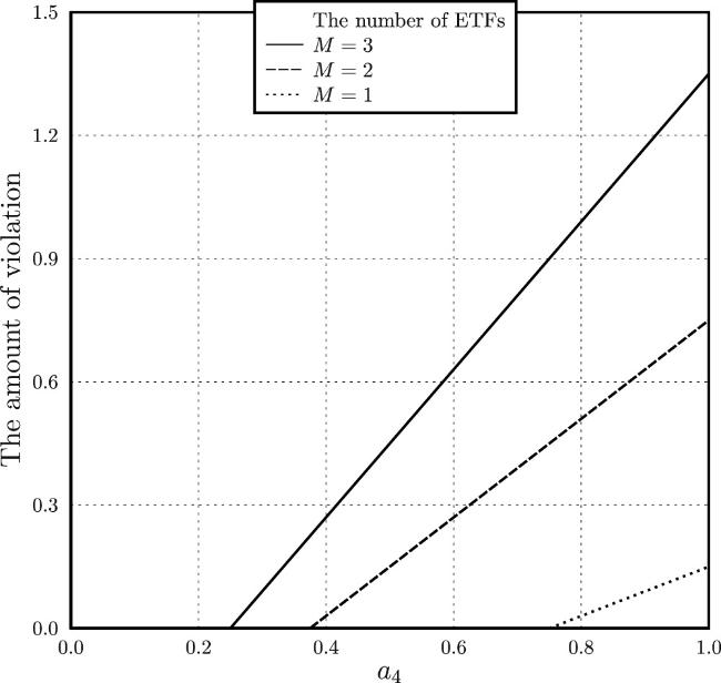
Such bipartite states were used to test new entanglement witnesses for 4 × 4 systems [65]. They concern the key problem to characterize boundaries between the entangled states and separable ones. Let us apply the correlation measure with mutually unbiased ETFs obtained from the matrices ϒ, Δϒ, Δ2ϒ, of which ϒ and Δ are described above by equations (13) and (14). Under the chosen circumstances, the region of detectability depends on the parameter a4. On the other hand, the detection power relies upon the number of involved ETFs. To characterize the situation, we will use the amount of violation defined as
$\begin{eqnarray}G\left({\tilde{{\boldsymbol{\sigma }}}}_{AB}\right)-\frac{(1-c)({d}^{2}-d)}{{n}^{2}}-\frac{M}{n}.\end{eqnarray}$
It shows how much the separability criterion (equation (24)) is violated. In figure 1, we depict the amount of violation with bipartite states of a pair of ququarts for M = 1, 2, 3. It is clearly seen that the detection power becomes stronger with growth of M. At the same time, the resulting improvement obtained with a pass from M = 1 to M = 2 is more essential, than with a pass from M = 2 to M = 3. It was already found for entanglement detection with a single ETF [32] that increasing the number of involved states improves the results. Thus, our findings are in a good agreement with the observations reported in the literature.
Figure 1. The amount of violation of the inequality (equation (24)) with bipartite states of the form (equation (46)) for M = 1, 2, 3.

4. Conclusions

This paper considered entanglement detection with the use of states from a mutually-unbiased-ETF. The well-known case of MUBs appeared here as an important particular one. Both the cases of bipartite and multipartite entanglement can be tested with the use of the presented criteria. There are several ways to pose separability criteria on the base of measurements assigned to a mutually-unbiased-ETF. One of them deals with the correlation measure originally developed with a set of MUBs. Mutually unbiased ETFs also lead to a family of positive maps, whence entanglement witnesses follow. In addition, criteria for tripartite and multipartite systems were derived. These criteria are formulated in terms of the Frobenius norm of the corresponding matrices. The presented findings have generalized the results obtained previously for a set of MUBs and for a single ETF. This paper additionally maintains the conclusion that applications of ETF-based measurements in quantum information science deserve more attention than they have obtained at the moment.

Appendix. Auxiliary calculations

This appendix aims to prove auxiliary statements concerning positive maps to build entanglement witnesses.

The map $\Psi$ expressed as equation (32) is positive and preserves the trace.

Let us begin with the fact that ${\boldsymbol{X}}\in {{ \mathcal L }}_{+}({{ \mathcal H }}_{d})$ implies ${\rm{\Psi }}({\boldsymbol{X}})\in {{ \mathcal L }}_{+}({{ \mathcal H }}_{d})$. It will be sufficient to prove here that [45]

$\begin{eqnarray}{\rm{tr}}\left[{\rm{\Psi }}{({\boldsymbol{X}})}^{2}\right]\leqslant \frac{1}{d-1},\end{eqnarray}$
for all X = ∣φ⟩⟨φ∣ with unit ket $| \varphi \rangle \in {{ \mathcal H }}_{d}$. This means that the output $\Psi$(X) lies in the largest ρ*-centered ball inscribed in the set of mixed states [50]. Immediate calculations show that
$\begin{eqnarray}\begin{array}{l}{\rm{tr}}\left[{\rm{\Psi }}{({\boldsymbol{X}})}^{2}\right]={\rm{tr}}\left[\frac{{{\mathbb{1}}}_{d}}{{d}^{2}}-\frac{2\eta }{d}\displaystyle \sum _{\mu =1}^{M}\displaystyle \sum _{i,j=1}^{n}{R}_{ij}^{(\mu )}{\rm{tr}}\left(\bar{{\boldsymbol{X}}}{{\boldsymbol{F}}}_{j}^{(\mu )}\right){{\boldsymbol{F}}}_{i}^{(\mu )}\right.\\ +\,{\eta }^{2}\displaystyle \sum _{\mu ,\nu =1}^{M}\displaystyle \sum _{i,j,k,\ell =1}^{n}\left.{R}_{ij}^{(\mu )}{\rm{tr}}\left(\bar{{\boldsymbol{X}}}{{\boldsymbol{F}}}_{j}^{(\mu )}\right){{\boldsymbol{F}}}_{i}^{(\mu )}{R}_{k\ell }^{(\nu )}{\rm{tr}}\left(\bar{{\boldsymbol{X}}}{{\boldsymbol{F}}}_{\ell }^{(\nu )}\right){{\boldsymbol{F}}}_{k}^{(\nu )}\Space{0ex}{3.85ex}{0ex}\right]\\ =\,\frac{1}{d}+\frac{{\eta }^{2}{d}^{2}}{{n}^{2}}\displaystyle \sum _{\mu ,\nu =1}^{M}\displaystyle \sum _{i,j,k,\ell =1}^{n}{R}_{ij}^{(\mu )}{R}_{k\ell }^{(\nu )}{\rm{tr}}\left(\bar{{\boldsymbol{X}}}{{\boldsymbol{F}}}_{j}^{(\mu )}\right){\rm{tr}}\left(\bar{{\boldsymbol{X}}}{{\boldsymbol{F}}}_{\ell }^{(\nu )}\right)\\ \times \,{\left|\langle {\phi }_{\mu i}| {\phi }_{\nu k}\rangle \right|}^{2}.\end{array}\end{eqnarray}$
The latter holds due to
$\begin{eqnarray*}\begin{array}{r}\begin{array}{l}\frac{2\eta }{n}\displaystyle \sum _{\mu =1}^{M}\displaystyle \sum _{i,j=1}^{n}{R}_{ij}^{(\mu )}{\rm{tr}}\left(\bar{{\boldsymbol{X}}}{{\boldsymbol{F}}}_{j}^{(\mu )}\right)=\frac{2\eta }{n}\displaystyle \sum _{\mu =1}^{M}\displaystyle \sum _{j=1}^{n}{\rm{tr}}\left(\bar{{\boldsymbol{X}}}{{\boldsymbol{F}}}_{j}^{(\mu )}\right)\\ =\,\frac{2\eta M}{n}\,{\rm{tr}}\left(\bar{{\boldsymbol{X}}}\right)=0,\end{array}\end{array}\end{eqnarray*}$
where we used the completeness relation and equation (30). The second term in the right-hand side of equation (A2) can be divided into the two sums, one of which for μ = ν and other for μ ≠ ν. The second sum is calculated as
$\begin{eqnarray}\begin{array}{l}\frac{{\eta }^{2}d}{{n}^{2}}\displaystyle \sum _{\mu \ne \nu }\displaystyle \sum _{i,j,k,\ell =1}^{n}{R}_{ij}^{(\mu )}{R}_{k\ell }^{(\nu )}{\rm{tr}}\left(\bar{{\boldsymbol{X}}}{{\boldsymbol{F}}}_{j}^{(\mu )}\right){\rm{tr}}\left(\bar{{\boldsymbol{X}}}{{\boldsymbol{F}}}_{\ell }^{(\nu )}\right)\\ =\,\frac{{\eta }^{2}d}{{n}^{2}}\displaystyle \sum _{\mu \ne \nu }\displaystyle \sum _{j,\ell =1}^{n}{\rm{tr}}\left(\bar{{\boldsymbol{X}}}{{\boldsymbol{F}}}_{j}^{(\mu )}\right){\rm{tr}}\left(\bar{{\boldsymbol{X}}}{{\boldsymbol{F}}}_{\ell }^{(\nu )}\right)\\ =\,\frac{{\eta }^{2}({M}^{2}-M)}{d}\,{\left[{\rm{tr}}\left(\bar{{\boldsymbol{X}}}\right)\right]}^{2}=0.\end{array}\end{eqnarray}$
The first sum reads as
$\begin{eqnarray}\begin{array}{l}{\eta }^{2}\displaystyle \sum _{\mu =1}^{M}\displaystyle \sum _{i,j,k,\ell =1}^{n}{R}_{ij}^{(\mu )}{R}_{k\ell }^{(\mu )}{\rm{tr}}\left(\bar{{\boldsymbol{X}}}{{\boldsymbol{F}}}_{j}^{(\mu )}\right){\rm{tr}}\left(\bar{{\boldsymbol{X}}}{{\boldsymbol{F}}}_{\ell }^{(\mu )}\right){\rm{tr}}({{\boldsymbol{F}}}_{i}^{(\mu )}{{\boldsymbol{F}}}_{k}^{(\mu )})\\ =\,\frac{{\eta }^{2}{d}^{2}}{{n}^{2}}\displaystyle \sum _{\mu =1}^{M}\displaystyle \sum _{i,j,\ell =1}^{n}{R}_{ij}^{(\mu )}{R}_{i\ell }^{(\mu )}{\rm{tr}}\left(\bar{{\boldsymbol{X}}}{{\boldsymbol{F}}}_{j}^{(\mu )}\right){\rm{tr}}\left(\bar{{\boldsymbol{X}}}{{\boldsymbol{F}}}_{\ell }^{(\mu )}\right)\\ +\,\frac{{\eta }^{2}c{d}^{2}}{{n}^{2}}\displaystyle \sum _{\mu =1}^{M}\displaystyle \sum _{i\ne k}\displaystyle \sum _{j,\ell =1}^{n}{R}_{ij}^{(\mu )}{R}_{k\ell }^{(\mu )}{\rm{tr}}\left(\bar{{\boldsymbol{X}}}{{\boldsymbol{F}}}_{j}^{(\mu )}\right){\rm{tr}}\left(\bar{{\boldsymbol{X}}}{{\boldsymbol{F}}}_{\ell }^{(\mu )}\right)\\ =\,\frac{{\eta }^{2}(1-c){d}^{2}}{{n}^{2}}\displaystyle \sum _{\mu =1}^{M}\displaystyle \sum _{j=1}^{n}{\left[{\rm{tr}}\left(\bar{{\boldsymbol{X}}}{{\boldsymbol{F}}}_{j}^{(\mu )}\right)\right]}^{2},\end{array}\end{eqnarray}$
due to the completeness relation and equation (31). Using $\bar{{\boldsymbol{X}}}={\boldsymbol{X}}-{{\boldsymbol{\rho }}}_{* }$, the right-hand side of equation (A4) can be rewritten as
$\begin{eqnarray}\begin{array}{r}\begin{array}{l}\frac{{\eta }^{2}(1-c){d}^{2}}{{n}^{2}}\left(\,\displaystyle \sum _{\mu =1}^{M}I({{ \mathcal F }}^{(\mu )};{\boldsymbol{X}})-\frac{M}{n}\right)\\ \quad \leqslant \,\frac{{\eta }^{2}{(1-c)}^{2}{d}^{3}(d-1)}{{n}^{4}}=\frac{1}{d(d-1)}.\end{array}\end{array}\end{eqnarray}$
Combining equation (A2) with equation (A5) results in
$\begin{eqnarray*}{\rm{tr}}\left[{\rm{\Psi }}{({\boldsymbol{X}})}^{2}\right]\leqslant \frac{1}{d}+\frac{1}{d(d-1)}=\frac{1}{d-1},\end{eqnarray*}$
due to equations (10) and (33). This completes the proof of the inequality (equation (A1)). It is immediate to check that the map of equation (32) preserves the trace.  

Let us prove the formula (37). The following statement was shown in reference [35]. If d2 unit vectors $| {\phi }_{j}\rangle \in {{ \mathcal H }}_{d}$ form a SIC-POVM then
$\begin{eqnarray}\displaystyle \frac{1}{{d}^{2}}\,\displaystyle \sum _{j=1}^{{d}^{2}}| {\phi }_{j}\rangle \langle {\phi }_{j}| \otimes | {\phi }_{j}\rangle \langle {\phi }_{j}| =\displaystyle \frac{2}{{d}^{2}+d}\,{{\boldsymbol{\Pi }}}_{\mathrm{sym}},\end{eqnarray}$
where Πsym is the orthogonal projection on the symmetric subspace of ${{ \mathcal H }}_{d}\otimes {{ \mathcal H }}_{d}$. Multiplying both the sides of equation (A6) by ${\boldsymbol{X}}\otimes {{\mathbb{1}}}_{d}$ and taking the partial trace over the first subsystem, we finally obtain equation (37). For every density matrix, it follows from equation (37) that
$\begin{eqnarray*}{\boldsymbol{\rho }}=(d+1)\displaystyle \sum _{j=1}^{{d}^{2}}{p}_{j}({ \mathcal N };{\boldsymbol{\rho }})\,| {\phi }_{j}\rangle \langle {\phi }_{j}| -{{\mathbb{1}}}_{d}.\end{eqnarray*}$
Thus, the use of measurement statistics allows one to recover the pre-measurement state. For informationally complete measurements, there is one-to-one correspondence between probability distributions and density matrices.
1
Horodecki R, Horodecki P, Horodecki M, Horodecki K 2009 Quantum entanglement Rev. Mod. Phys. 81 865-942

DOI

2
Gühne O, Tóth G 2009 Entanglement detection Phys. Rep. 474 1-75

DOI

3
Schrödinger E 1935 Die gegenwärtige situation in der quantenmechanik Naturwissenschaften 23 807-812

DOI

4
Einstein A, Podolsky B, Rosen N 1935 Can quantum-mechanical description of physical reality be considered complete? Phys. Rev. 47 777-780

DOI

5
Bohm D 1951 Quantum Theory Prentice-Hall

6
Deutsch D 1985 Quantum theory, the Church–Turing principle and the universal quantum computer Proc. R. Soc. Lond. A 400 97-117

DOI

7
Shor P W 1997 Polynomial-time algorithms for prime factorization and discrete logarithms on a quantum computer Soc. Ind. Appl. Math. J. Comput. 26 1484-1509

DOI

8
Grover L K 1997 Quantum mechanics helps in searching for a needle in a haystack Phys. Rev. Lett. 79 325-328

DOI

9
Grover L K 1997 Quantum computers can search arbitrarily large databases by a single query Phys. Rev. Lett. 79 4709-4712

DOI

10
Bennett C H, Bernstein E, Brassard G, Vazirani U 1997 Strengths and weaknesses of quantum computing SIAM J. Comput. 26 1510-1523

DOI

11
Wendin G 2017 Quantum information processing with superconducting circuits: a review Rep. Prog. Phys. 80 106001

DOI

12
Flamini F, Spagnolo N, Sciarrino F 2019 Photonic quantum information processing: a review Rep. Prog. Phys. 82 016001

DOI

13
Bruzewicz C D, Chiaverini J, McConnell R, Sage J M 2019 Trapped-ion quantum computing: progress and challenges Appl. Phys. Rev. 6 021314

DOI

14
Henriet L, Beguin L, Signoles A, Lahaye T, Browaeys A, Reymond G-O, Jurczak C 2020 Quantum computing with neutral atoms Quantum 4 327

DOI

15
Peres A 1996 Separability criterion for density matrices Phys. Rev. Lett. 77 1413-1415

DOI

16
Horodecki M, Horodecki P, Horodecki R 1996 Separability of mixed states: necessary and sufficient conditions Phys. Lett. A 223 1-8

DOI

17
Horodecki P 1997 Separability criterion and inseparable mixed states with positive partial transposition Phys. Lett. A 232 333-339

DOI

18
Horodecki M, Horodecki P, Horodecki R 2001 Separability of n-particle mixed states: necessary and sufficient conditions in terms of linear maps Phys. Lett. A 283 1-7

DOI

19
Yu X-D, Imai S, Gühne O 2021 Entanglement certification from moments of the partial transpose Phys. Lett. A 127 060504

DOI

20
Durt T, Englert B-G, Bengtsson I, Życzkowski K 2010 On mutually unbiased bases Int. J. Quantum Inf. 8 535-640

DOI

21
Zauner G 2011 Quantum designs: foundations of a noncommutative design theory Int. J. Quantum Inf. 9 445-507

DOI

22
Schwinger J 1960 Unitary operator bases Proc. Natl. Acad. Sci. U.S.A. 46 570-579

DOI

23
Ivanović I D 1981 Geometrical description of quantal state determination J. Phys. A: Math. Gen. 14 3241-3245

DOI

24
Wootters W K, Fields B D 1989 Optimal state-determination by mutually unbiased measurements Ann. Phys. 191 363-381

DOI

25
Bandyopadhyay S, Boykin P O, Roychowdhury V, Vatan F 2002 A new proof for the existence of mutually unbiased bases Algorithmica 34 512-528

DOI

26
Xiong Z-X, Shi H-D, Wang Y-N, Jing L, Lei J, Mu L-Z, Fan H 2012 General quantum key distribution in higher dimension Phys. Rev. A 85 012334

DOI

27
Fan H, Wang Y-N, Jing L, Yue J-D, Shi H-D, Zhang Y-L, Mu L-Z 2014 Quantum cloning machines and the applications Phys. Rep. 544 241-322

DOI

28
Scott A J 2006 Tight informationally complete quantum measurements J. Phys. A: Math. Gen. 39 13507

DOI

29
Rastegin A E 2024 Entropic uncertainty relations for measurements assigned to a projective two-design APL Quantum 1 026111

DOI

30
Rastegin A E 2023 Entropic uncertainty relations from equiangular tight frames and their applications Proc. R. Soc. A 479 20220546

DOI

31
Rastegin A E 2023 On Kirkwood–Dirac quasiprobabilities and unravelings of quantum channel assigned to a tight frame Physica A 629 129208

DOI

32
Shi X 2024 The entanglement criteria based on equiangular tight frames J. Phys. A: Math. Theor. 57 075302

DOI

33
van Lint J H, Seidel J J 1966 Equilateral point sets in elliptic geometry Indag. Math. 28 335-348

DOI

34
Lemmens P W H, Seidel J J 1973 Equiangular lines J. Algebra 24 494-512

DOI

35
Renes J M, Blume-Kohout R, Scott A J, Caves C M 2004 Symmetric informationally complete quantum measurements J. Math. Phys. 45 2171-2180

DOI

36
Fickus M, Mayo B R 2021 Mutually unbiased equiangular tight frames IEEE Trans. Inf. Theory 67 1656-1667

DOI

37
Rastegin A E 2024 Uncertainty relations for quantum coherence with respect to mutually unbiased equiangular tight frames Phys. Scr. 99 115109

DOI

38
Rastegin A E 2025 Kirkwood–Dirac quasiprobabilities for measurements related to mutually unbiased equiangular tight frames APL Quantum 2 026108

DOI

39
Pérez F C, Avella V G, Goyeneche D 2022 Mutually unbiased frames Quantum 6 851

DOI

40
Kalev A, Gour G 2014 Mutually unbiased measurements in finite dimensions New J. Phys. 16 053038

DOI

41
Siudzińska K 2024 Informationally overcomplete measurements from generalized equiangular tight frames J. Phys. A: Math. Theor. 57 335302

DOI

42
Spengler C, Huber M, Brierley S, Adaktylos T, Hiesmayr B C 2012 Entanglement detection via mutually unbiased bases Phys. Rev. A 86 022311

DOI

43
Rastegin A E 2013 Uncertainty relations for MUBs and SIC-POVMs in terms of generalized entropies Eur. Phys. J. D 67 269

DOI

44
Rastegin A E 2015 On uncertainty relations and entanglement detection with mutually unbiased measurements Open Syst. Inf. Dyn. 22 1550005

DOI

45
Chruściński D, Sarbicki G, Wudarski F 2018 Entanglement witnesses from mutually unbiased bases Phys. Rev. A 97 032318

DOI

46
Horn R A, Johnson C R 1990 Matrix Analysis Cambridge University Press

47
Nielsen M A, Chuang I L 2010 Quantum Computation and Quantum Information Cambridge University Press

48
D’Ariano G M, Perinotti P, Sacchi M F 2004 Informationally complete measurements and groups representation J. Opt. B: Quantum Semiclass. Opt. 6 S487-S491

DOI

49
Rastegin A E 2025 Uncertainty relations in terms of generalized entropies derived from information diagrams J. Phys. A: Math. Theor. 58 285303

DOI

50
Bengtsson I, Życzkowski K 2017 Geometry of Quantum States: An Introduction to Quantum Entanglement Cambridge University Press

51
Werner R F 1989 Quantum states with Einstein–Podolsky–Rosen correlations admitting a hidden-variable model Phys. Rev. A 40 4277-4281

DOI

52
Życzkowski K, Horodecki P, Sanpera A, Lewenstein M 1998 Volume of the set of separable states Phys. Rev. A 58 883-892

DOI

53
Waldron S F D 2018 An Introduction to Finite Tight Frames Birkhäuser

54
Kraus K 1987 Complementary observables and uncertainty relations Phys. Rev. D 35 3070-3075

DOI

55
Bennett C H, Brassard G 2014 Quantum cryptography: public key distribution and coin tossing Theor. Comput. Sci. 560 7-11

DOI

56
Davies E B 1978 Information and quantum measurement IEEE Trans. Inf. Theory 24 596-599

DOI

57
Peres A 1988 How to differentiate between non-orthogonal states Phys. Lett. A 128 19

DOI

58
Duan L-M, Guo G-C 1998 Probabilistic cloning and identification of linearly independent quantum states Phys. Rev. Lett. 80 4999-5002

DOI

59
Fan H 2004 Distinguishability and indistinguishability by local operations and classical communication Phys. Rev. Lett. 92 177905

DOI

60
Rastegin A E 2024 Uncertainty relations for quantum measurements from generalized equiangular tight frames Ann. Phys. 470 169785

DOI

61
Lewenstein M, Kraus B, Horodecki P, Cirac J 2001 Characterization of separable states and entanglement witnesses Phys. Rev. A 63 044304

DOI

62
Chruściński D, Sarbicki G 2014 Entanglement witnesses: construction, analysis and classification J. Phys. A: Math. Theor. 47 483001

DOI

63
Siudzińska K 2022 Indecomposability of entanglement witnesses constructed from symmetric measurements Sci. Rep. 12 10785

DOI

64
Horodecki M, Horodecki P 1999 Reduction criterion of separability and limits for a class of distillation protocols Phys. Rev. A 59 4206-4216

DOI

65
Jafarizadeh M A, Behzadi N, Akbari Y 2009 Entanglement witnesses and characterizing entanglement properties of some PPT states Eur. Phys. J. D 55 197-203

DOI

Outlines

/