


1. Introduction
Nuclear isomers, defined as metastable excited states of atomic nuclei, provide us with some unique opportunities for advancing our understanding of nuclear physics and astrophysics [1]. These long-lived excited states have attracted considerable research interest [2] over the past two decades due to their distinctive quantum mechanical properties and potential applications. Among various types of nuclear isomers, spin isomers, which arise from the difficulty in meeting spin selection rules, represent one of the most prevalent and extensively studied categories. The investigation of spin isomers holds particular significance in elucidating the fundamental properties of atomic nuclei, as well as promoting the development of nuclear experimental techniques.
Nuclei in the vicinity of the neutron number N = 50 and the proton number Z = 40 exhibit a remarkable abundance of spin isomers, presenting a fertile ground for nuclear structure studies. These isomeric states predominantly originate from either single-hole excitation from ν0g9/2 to ν1p1/2 or single-particle excitation from π1p1/2 to π0g9/2. The large differences in angular momentum (Δj = 4) between the first-excited state and the ground state create favorable conditions for the formation of long-lived isomeric states. The systematic investigation of spin isomers in this mass region can provide insights into both the underlying mechanisms of spin isomers and the shell structure properties around the double-closed-shell nucleus 90Zr.
While phenomenological theoretical approaches have been extensively employed to investigate spin isomers, the application of ab initio theoretical frameworks to isomeric state calculations remains rarely explored. The nuclear ab initio theory, which aims to solve the nuclear many-body problem from first principle using realistic nuclear interactions, represents the forefront of contemporary nuclear theoretical frameworks, offers the potential for parameter-free predictions of nuclear properties and could provide novel insights into the microscopic origins of isomers. Over the past two decades, remarkable advances have been achieved in ab initio many-body methods [3–6] with nuclear forces based on chiral effective field theory [7]. These developments have significantly expanded the reach of ab initio calculations to medium-mass nuclei, enabling the theoretical investigation of complex nuclear phenomena. The systematic uncertainties inherited in these calculations can now be quantified through order-by-order improvements in the chiral expansion, providing a rigorous framework for assessing theoretical predictions of nuclear observables, including spectroscopic properties relevant to isomeric states.
In the present work, we employ the ab initio many-body perturbation theory (MBPT) [8], which is one of the most powerful ab initio many-body methods, to systematically study the 1/2− spin isomer in the N = 49 isotones, including 83Se, 85Kr, 87Sr, 89Zr, 91Mo and 93Ru. The systematic study of isotones offers a unique probe to examine the evolution of single-particle properties, the robustness of shell closure and the microscopic mechanisms governing isomer formation. By analyzing these systems from an ab initio perspective, we can gain deeper insights into the influence of single-hole excitation on spin isomers in this mass region. Moreover, we use MBPT to study the decay properties, including M4 magnetic transitions and β decay, of these isomers consistently, giving good results.
2. Theory
2.1. Ab initio many-body perturbation theory
The intrinsic Hamiltonian of an A-nucleon system can be written as 1 ) in harmonic-oscillator (HO) basis, getting the HF basis. Then, we transferred the Hamiltonian (1 ) to the HF basis, and normal ordered it with respect to the HF reference state [10].
$\begin{eqnarray}H=\displaystyle \sum _{i=1}^{A}\left(1-\frac{1}{A}\right)\frac{{{\boldsymbol{p}}}_{i}^{2}}{2m}+\displaystyle \sum _{i\lt j}^{A}\left({v}_{ij}^{{\rm{NN}}}-\frac{{{\boldsymbol{p}}}_{i}\cdot {{\boldsymbol{p}}}_{j}}{mA}\right)+\displaystyle \sum _{i\lt j\lt k}^{A}{v}_{ijk}^{3{\rm{N}}},\end{eqnarray}$
where pi and pj are the nucleon momentum in the laboratory, m means the mass of the nucleon, and ${v}_{ij}^{{\rm{NN}}}$ and ${v}_{ijk}^{3{\rm{N}}}$ are the nucleon-nucleon (NN) and three-nucleon (3N) interactions, respectively. Due to the large cost of full inclusion of three-nucleon force (3NF) during ab initio many-body calculations, the normal-ordered two-body (NO2B) approximation [9] has been widely used in nuclear ab initio calculations to reduce the calculational cost. To do this, we first performed the Hartree–Fock (HF) calculation of the initial Hamiltonian (In this work, we used the ab initio MBPT [8] to construct the realistic valence-space effective Hamiltonian and other effective operators consistently for shell-model (SM) calculation. To do this, we separated the normal-ordered Hamiltonian into the one-body part H0 and the perturbative part H1 [11, 12]. The realistic valence-space effective interaction matrix elements for SM calculation was obtained by the so-called $\hat{Q}$-box folded diagrams [13]. Due to the non-degenerate property of the HF states, the extended Kuo–Krenciglowa method [14, 15] was used to build the effective Hamiltonian Heff. With the valence-space and its complementary-space projection operators P and Q, we iteratively solve the equation
$\begin{eqnarray}{H}_{{\rm{eff}}}^{(\kappa )}=P{H}_{0}P+\hat{Q}(\epsilon )+\displaystyle \sum _{n=1}^{\infty }\frac{1}{n!}\frac{{{\rm{d}}}^{n}\hat{Q}(\epsilon )}{{\rm{d}}{\epsilon }^{n}}{\left\{{H}_{{\rm{eff}}}^{(\kappa -1)}-\epsilon \right\}}^{n},\end{eqnarray}$
with κ being the κ-th iteration and the starting energy ε. The definition of $\hat{Q}$ box is $\begin{eqnarray}\hat{Q}(\epsilon )=P{H}_{1}P+P{H}_{1}Q\frac{1}{\epsilon -QHQ}Q{H}_{1}P,\end{eqnarray}$
with its derivatives $\begin{eqnarray}{\hat{Q}}_{n}(\epsilon )=\frac{1}{n!}\frac{{{\rm{d}}}^{n}\hat{Q}(\epsilon )}{{\rm{d}}{\epsilon }^{n}}.\end{eqnarray}$
The realistic valence-space single-particle energies are obtained by the so-called $\hat{S}$-box folded diagrams [16], which is defined as the one-body part of $\hat{Q}$ box. Both the $\hat{S}$ box and $\hat{Q}$ box are calculated up to the third order in this work.To calculate other observables of nuclei, we used the so-called $\hat{{\rm{\Theta }}}$ box [8] to renormalize the full-space operator Θ into the valence-space, getting the valence-space effective operator Θeff. The $\hat{{\rm{\Theta }}}$ box and their definition are defined as [8, 17]
$\begin{eqnarray}\hat{{\rm{\Theta }}}(\epsilon )=P{\rm{\Theta }}P+P{\rm{\Theta }}Q\frac{1}{\epsilon -QHQ}Q{H}_{1}P,\end{eqnarray}$
$\begin{eqnarray}\hat{{\rm{\Theta }}}({\epsilon }_{1};{\epsilon }_{2})=P{H}_{1}Q\frac{1}{{\epsilon }_{1}-QHQ}Q{\rm{\Theta }}Q\frac{1}{{\epsilon }_{2}-QHQ}Q{H}_{1}P,\end{eqnarray}$
and $\begin{eqnarray}{\hat{{\rm{\Theta }}}}_{n}=\frac{1}{n!}\frac{{{\rm{d}}}^{n}\hat{{\rm{\Theta }}}(\epsilon )}{{\rm{d}}{\epsilon }^{n}},\end{eqnarray}$
$\begin{eqnarray}{\hat{{\rm{\Theta }}}}_{mn}={\left.\frac{1}{m!n!}\frac{{{\rm{d}}}^{m}}{{\rm{d}}{\epsilon }_{1}^{m}}\frac{{{\rm{d}}}^{n}}{{\rm{d}}{\epsilon }_{2}^{n}}\hat{{\rm{\Theta }}}({\epsilon }_{1};{\epsilon }_{2})\right|}_{{\epsilon }_{1}={\epsilon }_{2}=\epsilon }.\end{eqnarray}$
The valence-space effective operator Θeff is defined as
$\begin{eqnarray}{{\rm{\Theta }}}_{{\rm{eff}}}=\displaystyle \sum _{\gamma ,\eta }| {\psi }_{\gamma }\rangle \langle {\widetilde{{\rm{\Psi }}}}_{\gamma }| {\rm{\Theta }}| {{\rm{\Psi }}}_{\eta }\rangle \langle {\widetilde{\psi }}_{\eta }| ,\end{eqnarray}$
where ∣$\Psi$γ⟩ means the full-space wave-function and ∣ψγ⟩ = P∣$\Psi$γ⟩ is the valence-space wave-function. With the $\hat{Q}$ box and $\hat{{\rm{\Theta }}}$ box, the effective operator Θeff can then be written as, $\begin{eqnarray}{{\rm{\Theta }}}_{{\rm{eff}}}={H}_{{\rm{eff}}}{\hat{Q}}^{-1}\left(\displaystyle \sum _{i}^{\infty }{\chi }_{i}\right),\end{eqnarray}$
where $\begin{eqnarray}\begin{array}{rcl}{\chi }_{0} & = & ({\hat{{\rm{\Theta }}}}_{0}+{\rm{h.c.}})+{\hat{{\rm{\Theta }}}}_{00}\\ {\chi }_{1} & = & ({\hat{{\rm{\Theta }}}}_{1}\hat{Q}+{\rm{h.c.}})+({\hat{{\rm{\Theta }}}}_{01}\hat{Q}+{\rm{h.c.}})\\ {\chi }_{2} & = & ({\hat{{\rm{\Theta }}}}_{1}{\hat{Q}}_{1}\hat{Q}+{\rm{h.c.}})+({\hat{{\rm{\Theta }}}}_{2}\hat{Q}\hat{Q}+{\rm{h.c.}})\\ & & +({\hat{{\rm{\Theta }}}}_{02}\hat{Q}\hat{Q}+{\rm{h.c.}})+\hat{Q}{\hat{{\rm{\Theta }}}}_{11}\hat{Q}.\\ & & \cdots \end{array}\end{eqnarray}$
In this work, we truncated the χi series at i = 2, which is sufficient for the convergence [8]. To be consistent with the Heff, the $\hat{{\rm{\Theta }}}$ box were also calculated up to the third order.2.2. Other operators
In the present work, we focused on the magnetic operator and Gamow–Teller β decay. In this subsection, we briefly introduce the basic equations and concepts of these operators. A more systematic introduction of these operators can be found in [18].
2.2.1. Magnetic operator
The tensor component of the full-space bare magnetic transition tensor operator Mλ is given by [18]12 ) being renormalized into the valence-space using the $\hat{{\rm{\Theta }}}$ box, we can get the expectation of the operator, i.e. $\langle {\psi }_{f}\parallel {\boldsymbol{M}}\lambda \parallel {\psi }_{i}\rangle $, with ψi and ψf being the wave functions of the initial and final state.
$\begin{eqnarray}{M}_{\lambda \mu }=\displaystyle \sum _{j=1}^{A}\left[\frac{2}{\lambda +1}{g}_{l}^{j}{{\boldsymbol{l}}}_{j}+{g}_{s}^{j}{{\boldsymbol{s}}}_{j}\right]\cdot {{\rm{\nabla }}}_{j}\left[{r}_{j}^{\lambda }{Y}_{\lambda \mu }({\hat{r}}_{j})\right],\end{eqnarray}$
where λ is the rank of the tensor operator [19], while lj and sj are the orbital and intrinsic angular momenta of the j-th nucleon, respectively. The values of g factors are taken from [18]. With the free-space bare operators (In this work, our main concerns are the magnetic moment and the reduced transition probability.
The magnetic moment of the state ∣ψJ⟩ is defined as
$\begin{eqnarray}\mu =\sqrt{\frac{4\pi }{3}}\sqrt{\frac{J}{(J+1)(2J+1)}}\langle {\psi }_{J}| | {\boldsymbol{M}}1| | {\psi }_{J}\rangle ,\end{eqnarray}$
with J being the total angular momentum of the state ∣ψJ⟩. For extreme single-particle or single-hole condition, the value of magnetic moment, also known as the Schmidt limit [20], can be obtained from the following equation, $\begin{eqnarray}{\mu }_{{\rm{sp}}}=\left\{\begin{array}{ll}{g}_{l}j+\frac{1}{2}\left({g}_{s}-{g}_{l}\right)\quad & \,\rm{for}\,\,\,j=l+\frac{1}{2},\\ {g}_{l}j-\left({g}_{s}-{g}_{l}\right)\frac{j}{2j+2}\,\quad & \,\rm{for}\,\,\,j=l-\frac{1}{2},\end{array}\right.\end{eqnarray}$
where j and l represent the total angular momentum and orbital angular momentum of the orbit of the single particle or single hole, gl and gs are the free-nucleon g-factors [18].The reduced transition probability is defined as
$\begin{eqnarray}B({\boldsymbol{M}}\lambda ;{\psi }_{i}\to {\psi }_{f})=\frac{1}{2{J}_{i}+1}| \langle {\psi }_{f}| | {\boldsymbol{M}}\lambda | | {\psi }_{i}\rangle {| }^{2},\end{eqnarray}$
with Ji being the angular momentum of the initial state. The transition probability can be calculated using $\begin{eqnarray}{T}_{i\to f}^{({\boldsymbol{M}}\lambda )}=\frac{2}{{\epsilon }_{0}\hslash }\frac{\lambda +1}{\lambda {[(2\lambda +1)!!]}^{2}}{\left(\frac{{E}_{\gamma }}{\hslash c}\right)}^{2\lambda +1}B\left({\boldsymbol{M}}\lambda ;{\psi }_{i}\to {\psi }_{f}\right),\end{eqnarray}$
where Eγ is the γ-decay energy from the state ψi to the state ψf in units of MeV. ε0 and ℏc are physics constants [18]. The partial half-life of the decay from ψi to ψf is calculated by $\begin{eqnarray}{t}_{1/2}^{i\to f}=\frac{{\mathrm{ln}}\,2}{{T}_{i\to f}}.\end{eqnarray}$
2.2.2. β decay
The full-space bare Fermi (F) and Gamow–Teller (GT) β decay operator are defined as [21]
$\begin{eqnarray}O(F)=\displaystyle \sum _{j}^{A}{\tau }_{\pm }^{j},\,O(GT)=\displaystyle \sum _{j}^{A}{\sigma }^{j}{\tau }_{\pm }^{j},\end{eqnarray}$
where σ stands for the Pauli spin operator and τ± are isospin operators corresponding to β± decays, respectively. We can then get the reduced F or GT transition matrix element [21] by $\begin{eqnarray}{M}_{{\rm{F}}}={\delta }_{{J}_{i}{J}_{f}}\displaystyle \sum _{p,q}{M}_{{\rm{F}}}^{p,q}\langle {\psi }_{f}| | \left[{a}_{p}^{\dagger }{a}_{q}\right]| | {\psi }_{i}\rangle ,\end{eqnarray}$
and $\begin{eqnarray}{M}_{{\rm{GT}}}=\displaystyle \sum _{p,q}{M}_{{\rm{GT}}}^{p,q}\langle {\psi }_{f}| | \left[{a}_{p}^{\dagger }{a}_{q}\right]| | {\psi }_{i}\rangle .\end{eqnarray}$
where Ji (Jf) is the angular momentum of the initial (final) state. p and q runs over all the index in the valence-space. It should be noted that for β− decay p must be proton index and q must be neutron index, while for β+ decay and electron capture (EC) the situation is opposite. ${M}_{{\rm{F}}}^{p,q}$ and ${M}_{{\rm{GT}}}^{p,q}$ are the valence-space effective F and GT transition matrix elements, respectively, derived from the full-space F and GT operator through the $\hat{{\rm{\Theta }}}$-box calculations.With the value of MF and MGT, we can calculate the F and GT reduced transition probabilities,
$\begin{eqnarray}{B}_{{\rm{F}}}=\frac{{g}_{{\rm{V}}}^{2}}{2{J}_{i}+1}{\left|{M}_{{\rm{F}}}\right|}^{2},\,{B}_{{\rm{GT}}}=\frac{{g}_{{\rm{A}}}^{2}}{2{J}_{i}+1}{\left|{M}_{{\rm{GT}}}\right|}^{2},\end{eqnarray}$
where Ji is the angular momentum of the initial state, while the factor gV and gA are the vector coupling constant of the weak interactions and the axial-vector coupling constant of the weak interactions [18], respectively. The half-life of the β decay from the initial state i to a final state f can be calculated by $\begin{eqnarray}{t}_{1/2}^{i\to f}=\frac{\kappa }{f\left({B}_{{\rm{F}}}+{B}_{{\rm{GT}}}\right)}.\end{eqnarray}$
where the constant κ = 6289 s [22], f is the phase factor [18].2.2.3. Half-life
Within the equations above, we can calculate the half-life of an initial state i by
$\begin{eqnarray}\frac{1}{{t}_{1/2}^{{\rm{total}}}}=\displaystyle \sum _{f}\frac{1}{{t}_{1/2}^{i\to f}}\end{eqnarray}$
where the sum runs over all the decay branches, including the electromagnetic transitions and β decays.3. Results and discussion
In the present work, we used the NN+3Nlnl [23, 24] with the NN interaction at N4LO [25] and the 3N interaction, which has the low-energy constants cD = −1.80, cE = −0.31 [23] and uses a mixture of local and non-local regulators [23, 24], as our input interaction. To speed up convergence, the NN and 3N interactions were consistently SRG evolved to the lower cutoff λSRG = 2.0 fm−1. This interaction can well reproduce the properties from light to medium-mass nuclei [23, 24, 26]. Additionally, the low-energy constants cD and cE in 3N force of the NN+3Nlnl interaction are constrained to the triton half-life and binding energy [23]. In [23] and [27], calculations using NN+3Nlnl can give better GT strength and B(M5) than using other forces, which would indicate that considering triton half-life would make the nuclear force better describe spin-dependent or isomorphic spin-dependent operators. The HO basis at ℏω = 16MeV with $e=2n+l\leqslant {e}_{{\rm{\max }}}=14$ was taken in our calculations, and we limited ${e}_{1}+{e}_{2}+{e}_{3}\leqslant {E}_{{\rm{3max}}}=24$ for 3NF. In [28], it has been demonstrated that the calculation with ${e}_{{\rm{\max }}}=14$ and ${E}_{{\rm{3max}}}=24$ can reach convergence for energies and other operators.
Using the MBPT, we have derived an effective shell-model Hamiltonian with the π(f5/2, p3/2, p1/2, g9/2) ⨂ ν(p1/2, g9/2, g7/2, d5/2) valence-space above 66Ni core for shell-model calculations. The shell-model calculation was performed using the large-scale shell-model code KSHELL [29]. As the large dimensions of the valence-space exceed the computational capacity of the supercomputer and the neutron excitations across N = 50 shell has been demonstrated to be very little in the low-lying states of the nuclei in this region in previous phenomenological shell-model calculations [30–34], we implement the truncation, which allows the valence protons to move freely among all the valence-proton orbits and a total of up to two neutrons to fill in the ν(g7/2, d5/2) orbits, in this work.
The spectra of N = 49 isotones and their daughter nuclei are given in figure 1. As can be seen in figure 1, we well reproduce the spectra of these nuclei. In [36], Cai has demonstrated that the 1/2− states in N = 50 isotones raise from the excitation of a single unpaired proton hole from π1p1/2 to π0g9/2. To illustrate the origin of 1/2− states in N = 49 isotones, we show the configurations of 9/2+ ground states and 1/2− states in these nuclei, as show in figure 2. In figure 2, we can find that a nuetron excite from ν1p1/2 to ν0g9/2 when nuclei excite from 9/2+ states to 1/2− states. However, the configurations are different between 9/2+ and 1/2− states in 83Se compared with other nuclei, as shown in figure 2(a), and this would be the origin the difference between the experimental and theoretical energy values of the 1/2− state of 83Se. From figure 2(a), we can find that as the number of protons increases, the valence protons gradually fill the π0f5/2, π1p3/2 and π1p1/2 orbits. The excitation on π0g9/2 orbit is the reason that magnetic moment of 89Zr deviate single-particle value. If we restrict the excitations on π0g9/2 orbit, theoretical magnetic moment of 89Zr is 0.613 μN, which is close to the Schmidt limit, 0.638 μN.
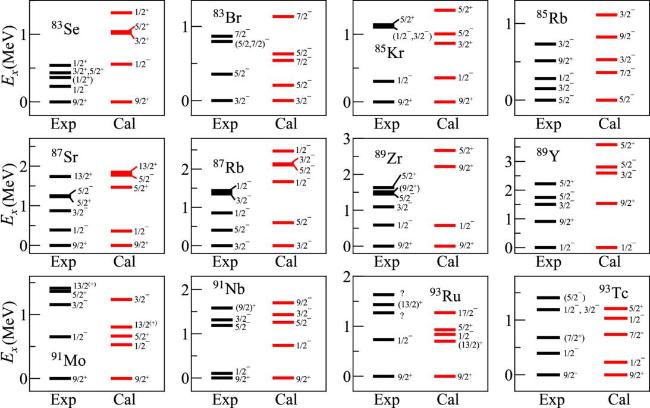
Figure 1. Spectra of N = 49 isotones and their daughter nuclei. Experimental data ara taken from [35]. The NN+3Nlnl interaction were used in the calculation. |
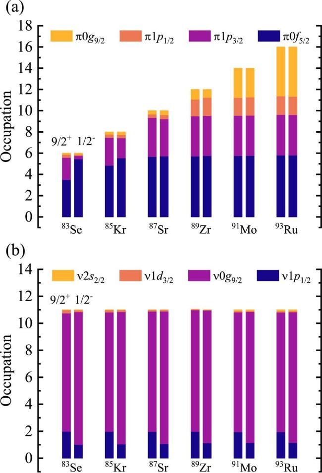
Figure 2. Configurations of 9/2+ states and 1/2− states in N = 49 isotones for proton orbits (a) and neutron orbits (b) in the valence-space. |
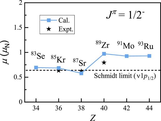
Since these 1/2− states of these nuclei can be considered to be caused by the excitation of a single unpaired neutron hole from ν1p1/2 to ν0g9/2, the states should have strong single-particle phenomena. To reveal this single-particle picture of 1/2− states, we have calculated the magnetic moment of them compared with experimental data [35] and the extreme single-particle magnetic moment of a neutron on the νp1/2 orbit which is the so-called 'Schmidt limit' [20], as can be seen in figure 3.
Figure 3. Nuclear magnetic moments for the 1/2− isomeric states of N = 49 isotones, compared with experimental data [35]. The horizontal dotted line means the single-particle value (Schmidt limit). |
In figure 3, it can be found that our calculation well reproduce the experimental data. The magnetic moments of 83Se, 85Kr and 87Sr are very close to the single-particle value, which reveal the robust single-particle characteristics in these three nuclei. However, for 89Zr, 91Mo and 93Ru, the values of the magnetic moments deviates slightly from the Schmidt limit for both experimental data and computational results. Our calculations also indicate that the magnetic moments of the 1/2− isomeric states in 91Mo and 93Ru are almost the same and both of them are slightly smaller than that of 89Zr.
To deeply understand the 1/2− states, we have also studied the decay properties of these states. We firstly calculated the reduced transition probabilities of the observed M4 transition of the 1/2− isomeric states, which is listed on table 1, compared with the experimental data. As can be found in figure 3, the calculated M4 reduced transition probabilities differs from the experimental data about 1.5 to 3 times. In addition to M4 magnetic transition, the 1/2− isomeric states can also decay through β transition.
Table 1. Calculated reduced transition probabilities B(M4) of the 1/2− isomers observed in N = 49 isotones in units of $1{0}^{5}{\mu }_{{\rm{N}}}^{2}{{\rm{fm}}}^{6}$. The NN+3Nlnl potentials are used. The experimental data is taken from [35]. |
| Nucleus | Transition | $B(M4)\,\left(1{0}^{5}{\mu }_{{\rm{N}}}^{2}{{\rm{fm}}}^{6}\right)$ | |
|---|---|---|---|
| Cal. | Expt. | ||
| 85Kr | ${\frac{1}{2}}^{-}\to {\frac{9}{2}}^{+}$ | 2.54 | 1.41(4) |
| 87Sr | 3.93 | 1.49(1) | |
| 89Zr | 4.41 | 1.58(1) | |
| 91Mo | 3.41 | 1.27(4) | |
| 93Ru | 2.77 | 1.18(14) | |
Tables 2 and 3 give the theoretical results of Fermi and Gamow–Teller reduced transition probabilities, along with computational and experimental ${\mathrm{log}}\,ft$ values of all the observed β-decay branch of the 1/2− isomeric states which we studied. It should be noted that due to the selection rules for allowed beta decay transitions, the values of B(F) are theoretically equal to zero when the Jπ of the final state is 3/2−. The Fermi operator connects isobaric analog states [37], which means that the initial state and final state of a β decay can been seen as isobaric analog states with each other if B(F) is much larger than B(GT). As can be seen in the two tables, we can find that, for those branches whose final states are Jπ = 1/2− on experiment, our calculations give B(GT) values that are bigger than B(F), which means that these states are isospin-mixed states and the isobaric analog component are smaller than the isobaric non-analog component. However, for the branches whose final states are degenerate with Jπ being 1/2− and 3/2− on experiment, except for two branches of 83mSe with the final states being 83Br$\,\left({\frac{1}{2}}_{2}^{-},{\frac{3}{2}}_{3}^{-}\right)$ and 83Br$\,\left({\frac{1}{2}}_{4}^{-},{\frac{3}{2}}_{6}^{-}\right)$ on experiment, our calculations give similar B(F) and B(GT) values for the final state with Jπ = 1/2− on theory, which indicates that the proportions of the isobaric analog component and isobaric non-analog component are similar in these states. Additionally, our results show that the decay branches of 83mSe, whose the final states are 83Br$\,\left({\frac{1}{2}}_{2}^{-},{\frac{3}{2}}_{3}^{-}\right)$ and 83Br$\,\left({\frac{1}{2}}_{4}^{-},{\frac{3}{2}}_{6}^{-}\right)$ on experiment, have strong B(F) values compared with B(GT) for the final state with Jπ = 1/2− on theory, which can be seen in table 2, demonstrating strong isobaric analog component in these two decay branches.
Table 2. Calculated β-decay reduced transition probabilities and calculated and experimental ${\mathrm{log}}\,ft$ values of the 1/2− isomers observed in 83Se, 85Kr and 87Sr. The NN+3Nlnl potentials are used. The experimental data is taken from [35]. |
| Transition | B(F) | B(GT) | ${\mathrm{log}}\,ft$ | |||
|---|---|---|---|---|---|---|
| Initial(Jπ) | Final(Jπ) | Expt. | Cal. | |||
| Expt. | Cal. | |||||
| 83Se(${\frac{1}{2}}_{1}^{-}$) | 83Br$\left({\frac{3}{2}}_{1}^{-}\right)$ | 83Br$\left({\frac{3}{2}}_{1}^{-}\right)$ | 0 | 7.29×10⁻⁴ | 6.0(1) | 6.9 |
| 83Br$\left({\frac{1}{2}}_{2}^{-},{\frac{3}{2}}_{3}^{-}\right)$ | 83Br$\left({\frac{1}{2}}_{2}^{-}\right)$ | 2.79×10⁻² | 4.12×10⁻⁴ | 5.8(1) | 5.3 | |
| 83Br$\left({\frac{3}{2}}_{3}^{-}\right)$ | 0 | 1.42×10⁻² | 5.6 | |||
| 83Br$\left({\left(\frac{3}{2}\right)}_{4}^{-}\right)$ | 83Br$\left({\frac{3}{2}}_{4}^{-}\right)$ | 0 | 2.30×10⁻³ | 5.4(1) | 6.4 | |
| 83Br$\left({\frac{1}{2}}_{3}^{-},{\frac{3}{2}}_{5}^{-}\right)$ | 83Br$\left({\frac{1}{2}}_{3}^{-}\right)$ | 2.31×10⁻⁴ | 5.76×10⁻⁴ | 7.3(1) | 6.9 | |
| 83Br$\left({\frac{3}{2}}_{5}^{-}\right)$ | 0 | 3.33×10⁻³ | 6.3 | |||
| 83Br$\left({\frac{1}{2}}_{4}^{-},{\frac{3}{2}}_{6}^{-}\right)$ | 83Br$\left({\frac{1}{2}}_{4}^{-}\right)$ | 2.72×10⁻⁵ | 4.25×10⁻⁷ | 6.0(1) | 8.4 | |
| 83Br$\left({\frac{3}{2}}_{6}^{-}\right)$ | 0 | 1.12×10⁻² | 5.7 | |||
| 83Br$\left({\frac{1}{2}}_{5}^{(-)},{\frac{3}{2}}_{8}\right)$ | 83Br$\left({\frac{1}{2}}_{5}^{-}\right)$ | 2.41×10⁻⁴ | 5.99×10⁻⁴ | 5.9(1) | 6.9 | |
| 83Br$\left({\frac{3}{2}}_{8}^{-}\right)$ | 0 | 2.76×10⁻⁴ | 7.4 | |||
| 83Br$\left({\frac{1}{2}}_{6}^{-},{\frac{3}{2}}_{9}^{-}\right)$ | 83Br$\left({\frac{1}{2}}_{6}^{-}\right)$ | 1.36×10⁻³ | 2.51×10⁻³ | 4.8(1) | 6.2 | |
| 83Br$\left({\frac{3}{2}}_{9}^{-}\right)$ | 0 | 1.86×10⁻² | 5.5 | |||
| 83Br$\left({\frac{1}{2}}_{10}^{-},{\frac{3}{2}}_{13}^{-}\right)$ | 83Br$\left({\frac{1}{2}}_{10}^{-}\right)$ | 8.28×10⁻³ | 8.75×10⁻³ | 5.9(4) | 5.6 | |
| 83Br$\left({\frac{3}{2}}_{13}^{-}\right)$ | 0 | 2.75×10⁻³ | 6.4 | |||
| 83Br$\left({\frac{1}{2}}_{11}^{-},{\frac{3}{2}}_{14}^{-}\right)$ | 83Br$\left({\frac{1}{2}}_{11}^{-}\right)$ | 3.60×10⁻² | 4.40×10⁻² | 5.7(1) | 4.9 | |
| 83Br$\left({\frac{3}{2}}_{14}^{-}\right)$ | 0 | 8.53×10⁻² | 4.9 | |||
| 85Kr$\left({\frac{1}{2}}_{1}^{-}\right)$ | 85Rb$\left({\frac{3}{2}}_{1}^{-}\right)$ | 85Rb$\left({\frac{3}{2}}_{1}^{-}\right)$ | 0 | 5.71×10⁻² | 7.1(1) | 5.042 |
| 85Rb$\left({\frac{1}{2}}_{1}^{-}\right)$ | 85Rb$\left({\frac{1}{2}}_{1}^{-}\right)$ | 4.17×10⁻⁵ | 6.51×10⁻⁴ | 7.39(2) | 6.96 | |
| 85Rb$\left({\frac{3}{2}}_{2}^{-}\right)$ | 85Rb$\left({\frac{3}{2}}_{2}^{-}\right)$ | 0 | 2.98×10⁻⁵ | 5.250(8) | 8.325 | |
| 87Sr$\left({\frac{1}{2}}_{1}^{-}\right)$ | 87Rb$\left({\frac{3}{2}}_{1}^{-}\right)$ | 87Rb$\left({\frac{3}{2}}_{1}^{-}\right)$ | 0 | 1.51 | 4.40(12) | 3.62 |
Table 3. Same as table 2 but for 1/2− isomers in 89Zr, 91Mo and 93Ru. |
| Transition | B(F) | B(GT) | ${\mathrm{log}}\,ft$ | |||
|---|---|---|---|---|---|---|
| Initial(Jπ) | Final(Jπ) | Expt. | Cal. | |||
| Expt. | Cal. | |||||
| 89Zr$\left({\frac{1}{2}}_{1}^{-}\right)$ | 89Y$\left({\frac{1}{2}}_{1}^{-}\right)$ | 89Y$\left({\frac{1}{2}}_{1}^{-}\right)$ | 1.23×10⁻² | 3.36×10⁻² | 7.1(4) | 5.1 |
| 89Y$\left({\frac{3}{2}}_{1}^{-}\right)$ | 89Y$\left({\frac{3}{2}}_{1}^{-}\right)$ | 0 | 1.63 | 4.31(2) | 3.59 | |
| 91Mo$\left({\frac{1}{2}}_{1}^{-}\right)$ | 91Nb$\left({\frac{1}{2}}_{1}^{-}\right)$ | 91Nb$\left({\frac{1}{2}}_{1}^{-}\right)$ | 7.56×10⁻³ | 2.88×10⁻² | 5.94(22) | 1.27(4) |
| 91Nb$\left({\frac{3}{2}}_{1}^{-}\right)$ | 91Nb$\left({\frac{3}{2}}_{1}^{-}\right)$ | 0 | 3.31×10⁻³ | 4.78(4) | ||
| 91Nb$\left({\frac{3}{2}}_{2}^{-}\right)$ | 91Nb$\left({\frac{3}{2}}_{2}^{-}\right)$ | 0 | 1.54 | 4.4(4) | ||
| 91Nb$\left({\left(\frac{3}{2}\right)}_{3}^{-}\right)$ | 91Nb$\left({\frac{3}{2}}_{3}^{-}\right)$ | 0 | 5.11×10⁻³ | 5.03(4) | ||
| 93Ru$\left({\frac{1}{2}}_{1}^{-}\right)$ | 93Tc$\left({\frac{1}{2}}_{1}^{-}\right)$ | 93Tc$\left({\frac{1}{2}}_{1}^{-}\right)$ | 1.27×10⁻² | 3.93×10⁻² | >5.6 | 5.1 |
| 93Tc$\left({\frac{1}{2}}_{3}^{-},{\frac{3}{2}}_{2}^{-}\right)$ | 93Tc$\left({\frac{1}{2}}_{3}^{-}\right)$ | 1.20×10⁻² | 1.05×10⁻² | 4.84(3) | 5.45 | |
| 93Tc$\left({\frac{3}{2}}_{2}^{-}\right)$ | 0 | 2.28×10⁻³ | 6.44 | |||
| 93Tc$\left({\frac{1}{2}}_{4}^{-},{\frac{3}{2}}_{3}^{-}\right)$ | 93Tc$\left({\frac{1}{2}}_{4}^{-}\right)$ | 9.29×10⁻³ | 2.93×10⁻³ | 4.526(19) | 5.712 | |
| 93Tc$\left({\frac{3}{2}}_{3}^{-}\right)$ | 0 | 1.38 | 3.658 | |||
| 93Tc$\left({\left({\frac{1}{2}}_{5},{\frac{3}{2}}_{4}\right)}^{-}\right)$ | 93Tc$\left({\frac{1}{2}}_{4}^{-}\right)$ | 1.75×10⁻² | 3.51×10⁻³ | 4.72(3) | 5.48 | |
| 93Tc$\left({\frac{3}{2}}_{4}^{-}\right)$ | 0 | 3.16×10⁻² | 5.30 | |||
| 93Tc$\left({\left(\frac{3}{2}\right)}_{5}^{-}\right)$ | 93Tc$\left({\frac{3}{2}}_{5}^{-}\right)$ | 0 | 2.06×10⁻³ | ≤4.7 | 6.5 | |
With the values in tables 1, 2 and 3, we also calculated the half-life of these 1/2− isomers using equation (17 ), (22 ) and (23 ), which are given in table 4. Because the calculation result of half-life is very sensitive to the electromagnetic transition energy Eγ and Q values of β decay, we use the experimental value [35] in the half-life calculation. It can be seen from table 4 that our calculations and experimental results are in very good agreement, showing the reliability of ab initio calculations in description of spin isomers.
Table 4. Calculated half-life of the 1/2− isomers in N = 49 isotones, compared with experimental [35]. |
| Nucleus | half-life | |
|---|---|---|
| Cal. | Expt. | |
| 83Se | 2.74 min | 1.17(1) min |
| 85Kr | 6.197 h | 4.480(8) h |
| 87Sr | 3.645 h | 2.815(12) h |
| 89Zr | 32.638 min | 4.161(12) min |
| 91Mo | 76.1 s | 65.0(7) s |
| 93Ru | 7.4 s | 10.8(3) s |
4. Summary
We have performed ab initio calculations for the N = 49 isotones. We have derived the valence-space effective Hamiltonian and other effective operators with the chiral two- plus three-nucleon force NN+3Nlnl using the $\hat{Q}$-box and $\hat{{\rm{\Theta }}}$-box folded diagrams, respectively, with the 66Ni core. With the valence-space effective Hamiltonian and operators, we have investigated the magnetic moments and the decay properties of isomers of the N = 49 isotones.
We first calculate the energies and the magnetic moments of the 1/2− isomers o N = 49 isotones. Our calculations reproduce reasonably experimental data and revealed the strong single-particle phenomena in 83Se, 85Kr and 87Sr. We then focus on the decay properties of the isomers we studied, including M4 magnetic transitions and β-decay properties. Our calculations can give good results of these properties, demonstrating the reliability of ab initio theory of studying the structure and decay properties of spin isomers in A ≈ 90 mass region.