


1. Introduction
Over the past century, black holes (BHs) have transformed from purely mathematical curiosities to observationally confirmed astrophysical objects with the landmark detection of gravitational waves from binary BH mergers by LIGO-Virgo collaborations [1, 2] and the groundbreaking first image of a BH shadow by the Event Horizon Telescope [3]. In the framework of classical general relativity (GR), the Kerr–Newman family of BHs, characterized by just three parameters—mass, charge and angular momentum—stands as the unique solution to Einstein’s field equations under the no-hair theorem [4, 5]. However, this theorem faces challenges when considering quantum effects, modified gravity theories or the presence of topological defects in the BH spacetime.
Among various BH solutions beyond the classical paradigm, the Frolov BH has gained significant attention in recent years [6]. Introduced by V P Frolov in 2016, this non-singular BH model represents an important advance in addressing the longstanding singularity problem in BH physics. The Frolov BH incorporates a length scale parameter α (related to the Hubble length) that regulates the central singularity through a specific coupling between electromagnetic (EM) and gravitational fields. Unlike conventional Reissner–Nordström (RN) BHs, which contain a physical singularity at r = 0, the Frolov model employs a radially dependent mass function that effectively smooths out the central region, thereby avoiding the infinite curvature problem [7, 8]. This model is particularly valuable since it preserves the horizon structure and many thermodynamic properties of classical BHs while eliminating the troublesome singularity that conflicts with quantum principles [9].
Topological defects, as relics of symmetry-breaking phase transitions in the early universe, provide another rich arena for extending BH physics beyond standard models. Global monopole (GM), first investigated by Barriola et al [10], represents topological defects arising from the spontaneous breaking of global O(3) symmetry to U(1). The spacetime around a GM exhibits a solid deficit angle and modified gravitational potential, creating distinctive effects on geodesic motion and causal structure [11, 12]. Similarly, cosmic strings are 1D topological defects resulting from the breaking of U(1) symmetry, which produces a conical deficit angle in the surrounding spacetime [13]. Both GM and a cloud of strings (CS) have been extensively studied for their cosmological implications, from structure formation to gravitational lensing effects [14, 15], and their incorporation into BH spacetimes introduces remarkable physical behavior not present in standard solutions. Let us briefly consider this static and spherically symmetric BH spacetime with a GM, formed through the spontaneous symmetry-breaking of a triplet of scalar fields ψi (i = 1, 2, 3), possessing a global SO(3) symmetry. The action that gives rise to the GM solution is given in [10] as,
$\begin{eqnarray}\begin{array}{rcl}S & = & \displaystyle \int {{\rm{d}}}^{4}x\sqrt{-g}\\ & & \times \left[R-\frac{1}{2}\,{g}^{\mu \nu }({\partial }_{\mu }{\psi }^{i})({\partial }_{\nu }{\psi }^{i})-\frac{\lambda }{4}{({\psi }^{i}\,{\psi }^{i}-{\eta }^{2})}^{2}\right],\end{array}\end{eqnarray}$
where η is the energy scale of symmetry-breaking and λ is a constant.As outlined in the original work [10], a monopole can be described through the following ansatz:
$\begin{eqnarray}{\psi }^{i}=\frac{\eta \,f(r)\,{x}^{i}}{r},\quad \quad {x}^{i}\,{x}^{i}={r}^{2}.\end{eqnarray}$
We consider a general static and spherical symmetric metric of the following form: $\begin{eqnarray}{\rm{d}}{s}^{2}=-B(r)\,{\rm{d}}{t}^{2}+A(r)\,{\rm{d}}{r}^{2}+{r}^{2}\,({\rm{d}}{\theta }^{2}+{\sin }^{2}\theta \,{\rm{d}}{\phi }^{2}).\end{eqnarray}$
Using this, one can find that the field equations for the scalar fields ψi can be reduced to a single equation for f(r) as follows: $\begin{eqnarray}\begin{array}{l}\frac{{f}^{{\prime\prime} }(r)}{A(r)}+\left[\frac{2}{r\,A(r)}+\frac{1}{2\,B(r)}\,{\left(\frac{B(r)}{A(r)}\right)}^{{\prime} }\right]\,{f}^{{\prime} }(r)\\ \,-\frac{2\,f(r)}{{r}^{2}}-\lambda \,{\eta }^{2}\,f(r)\,({f}^{2}(r)-1)=0,\end{array}\end{eqnarray}$
where prime denotes partial derivative w. r. t. r.Moreover, the energy-momentum tensor for the spacetime with a GM can be expressed as,
$\begin{eqnarray}{T}_{t}^{t}=\frac{{\eta }^{2}\,{f{}^{{\prime} }}^{2}(r)}{2\,A}+\frac{{\eta }^{2}\,{f}^{2}(r)}{{r}^{2}}+\frac{\lambda }{4}\,{\eta }^{4}\,{({f}^{2}(r)-1)}^{2},\end{eqnarray}$
$\begin{eqnarray}{T}_{r}^{r}=-\frac{{\eta }^{2}\,{f{}^{{\prime} }}^{2}(r)}{2\,A}+\frac{{\eta }^{2}\,{f}^{2}(r)}{{r}^{2}}+\frac{\lambda }{4}\,{\eta }^{4}\,{({f}^{2}(r)-1)}^{2},\end{eqnarray}$
$\begin{eqnarray}{T}_{\theta }^{\theta }={T}_{\phi }^{\phi }=\frac{{\eta }^{2}\,{f{}^{{\prime} }}^{2}(r)}{2\,A}+\frac{\lambda }{4}\,{\eta }^{4}\,{({f}^{2}(r)-1)}^{2}.\end{eqnarray}$
One can take the approximation a(r) = 1 outside the core due to the fact that a(r) grows linearly when r < δ and tends exponentially to unity as soon as r > δ, where $\delta \sim {(\eta \,\sqrt{\lambda })}^{-1}$ is the core radius. With this approximation, the energy-momentum tensor has a very simple form. It is given by, $\begin{eqnarray}{T}_{\nu }^{\mu }\approx \left(\frac{{\eta }^{2}}{{r}^{2}},\,\frac{{\eta }^{2}}{{r}^{2}},\,0,\,0\right).\end{eqnarray}$
And one can obtain a GM solution of the Einstein field equations where the metric function is given by, $\begin{eqnarray}B(r)={A}^{-1}(r)=1-8\,\pi \,{\eta }^{2}-\frac{2\,M}{r},\end{eqnarray}$
where M is a constant of integration and in flat space M ∼ Mcore, the mass of monopole core. For a detailed analysis of the physics associated with the GM spacetime, readers are referred to [10].The integration of these topological defects with BH solutions has led to compelling composite spacetime structures. Various authors extended BHs with GM in the literature [10, 16, 17]. Similarly, BHs threaded by CS have been investigated for their modified properties compared to their standard counterparts [18, 19]. These composite solutions are not merely theoretical constructs but represent plausible astrophysical configurations that could form through various evolutionary pathways in the early universe [20]. The combined Frolov BH with dual topological defects (GM and CS), as studied in this paper, therefore represents a physically motivated extension that incorporates both non-singular behavior and topological effects into a unified spacetime structure. Namely, this composite BH model is physically motivated by realistic astrophysical scenarios where BHs form in early universe environments rich in topological defects from phase transitions. These BHs could inherit both GM and CS signatures during primordial formation or through subsequent accretion of topological matter [19, 20]. The Frolov regularization provides a self-consistent framework that avoids singularities while preserving the essential physics needed to study how these inherited topological features manifest in observable quantities such as shadows and gravitational wave signals.
BH thermodynamics constitutes one of the most profound connections between gravity, quantum theory and information science. Since Hawking’s seminal discovery that BHs emit thermal radiation with a temperature proportional to their surface gravity [21, 22], the thermodynamic properties of BHs have been extensively analyzed. The four laws of BH thermodynamics, formulated by Bardeen, Carter and Hawking [23], establish direct analogies between BH physics and conventional thermodynamics, with the BH mass, horizon area and surface gravity corresponding to energy, entropy and temperature, respectively. These thermodynamic properties serve as crucial probes of a BH’s stability, phase transitions and information-theoretic characteristics [24, 25]. For modified BH solutions such as the Frolov BH with GM and CS, the thermodynamic analysis becomes particularly revealing since it can identify unique behavior that distinguishes these solutions from standard BHs and potentially lead to observable signatures [26].
The BH shadow, a dark region against a bright background as viewed by a distant observer, represents one of the few directly observable features of BHs. The shadow’s size and shape depend sensitively on the BH’s mass, spin and the underlying spacetime geometry [27]. Following the groundbreaking observations by the Event Horizon Telescope collaboration [3], BH shadow studies have evolved from theoretical curiosities to powerful tools for testing GR and alternative gravity theories [28, 29]. The shadow of non-standard BH, such as the Frolov BH with GM and CS, can exhibit distinctive features that potentially allow for observational discrimination between different theoretical models [30, 31]. The shadow calculation involves determining the photon sphere, a region where light rays can orbit the BH in unstable circular orbits, which marks the boundary between photons that escape to infinity and those captured by the BH [32]. The dynamical and shadow properties of BHs with CS and GM have previously been investigated in the literature for Schwarzschild and RN spacetimes [16–19]. Our combined Frolov-GM-CS model exhibits both similarities and distinctive differences compared to these earlier studies, particularly in the opposing effects of regularization versus topological defect parameters on shadow radius and quasinormal mode (QNM) spectra.
The study of perturbations around BH spacetime provides crucial insights into their stability and response to external disturbances. Scalar, EM and gravitational perturbations induce characteristic oscillations known as QNMs, which have specific frequencies and damping times determined by the BH parameters [33, 34]. These QNMs not only probe the stability of the underlying spacetime but also carry distinctive 'fingerprints' of the BH’s fundamental properties and offer a direct observational window into BH physics [35–38]. In the context of gravitational wave astronomy, QNMs manifest in the ringdown phase following BH mergers, offering a direct observational window into BH physics [39, 40].
The motivation for studying the Frolov BH with GM and CS stems from several compelling factors. First, the synthesis of non-singular BH models with topological defects represents a natural theoretical progression that addresses both the singularity problem and the influence of early universe phase transitions on BH formation and evolution. Second, the increasing precision of astrophysical observations, particularly in gravitational wave astronomy and BH imaging, creates opportunities for testing extended BH models against observational data. Third, the composite solutions, from modified thermodynamic behavior to distinctive shadow characteristics and perturbation spectra, serve as important test beds for exploring potential signatures of quantum gravity or modified gravity theories in the strong-field regime [41, 42]. In this paper, we conduct a comprehensive investigation of the Frolov BH with GM and CS, focusing on its geometric, thermodynamic and perturbative properties. We systematically analyze how the four key parameters of the model—the length scale parameter α, the charge q, the GM parameter η and the CS parameter a—influence various physical characteristics of the spacetime. Our analysis reveals several notable features: (1) the presence of GM and CS significantly modifies the horizon structure and thermodynamic stability, (2) the shadow radius exhibits opposing trends with respect to the Frolov parameters versus the topological defect parameters, and (3) the QNM spectrum shows distinctive patterns that potentially allow for observational discrimination of this model from ordinary GR BHs. Throughout our analysis, we emphasize the physical implications of these findings and their potential observational signatures.
The paper is organized as follows. In section 2 , we introduce the Frolov BH with GM and CS, examining its metric structure and horizon properties. We study the dynamics of photons in the geometry of Frolov BH with GM and CS in section 3 . Section 4 is devoted to a detailed analysis of the BH’s thermodynamic characteristics, including mass, temperature, entropy and heat capacity functions. In section 5 , we investigate the BH shadow, calculating the photon sphere and shadow radius for various parameter configurations. Section 6 focuses on scalar and EM perturbations, deriving the effective potential and computing the QNM frequencies using the Wentzel–Kramers–Brillouin (WKB) approximation. Finally, in section 7 , we summarize our findings and discuss their implications for theoretical and observational BH physics. Throughout the paper, we adopt natural units where G = c = ℏ = kB = 1.
2. Features of the Frolov BH with GM and CS
The Frolov BH represents a significant advancement in addressing the central singularity problem that plagues classical BH solutions [9, 43]. When combined with topological defects, such as a GM and a CS, the resulting spacetime exhibits rich physical properties that merit detailed investigation. In this section, we analyze the fundamental features of the Frolov BH with GM and CS, focusing on its metric structure, total action and horizon characteristics.
We begin by formulating the complete action that governs the Frolov BH spacetime, incorporating both a GM and a CS, along with a nonlinear electromagnetic field minimally coupled to gravity. This model draws from the regular charged BH framework developed in [6], where nonlinear electrodynamics (NLED) replaces the standard Maxwell theory to ensure regularity of the central curvature. The total action reads:
$\begin{eqnarray}\begin{array}{rcl}{S}_{{\rm{total}}} & = & \frac{1}{16\pi }\displaystyle \int {{\rm{d}}}^{4}x\sqrt{-g}\left[R+16\pi {{ \mathcal L }}_{{\rm{NLED}}}\right.\\ & & -8\pi \left.\left({\partial }_{\mu }{\phi }^{i}{\partial }^{\mu }{\phi }^{i}+\frac{\lambda }{2}{({\phi }^{i}{\phi }^{i}-{\eta }^{2})}^{2}\right)\right]+{S}^{{\rm{CS}}},\end{array}\end{eqnarray}$
where g is the determinant of the metric gμν, R is the Ricci scalar and ${{ \mathcal L }}_{{\rm{NLED}}}$ is the nonlinear electromagnetic Lagrangian. The scalar field φi (i = 1, 2, 3) represents the GM field, with symmetry-breaking scale η and self-coupling λ. In the broken symmetry vacuum, the limit λ → ∞ enforces φiφi = η2, inducing a solid-angle deficit. The term SCS accounts for the CS, described below.The energy-momentum tensor for the CS takes the form [13]:
$\begin{eqnarray}\begin{array}{l}{T}_{t}^{t\,(CS)}={T}_{r}^{r\,(CS)}={\rho }_{c}=\frac{a}{{r}^{2}},\\ {T}_{\theta }^{\theta \,(CS)}={T}_{\phi }^{\phi \,(CS)}=0,\end{array}\end{eqnarray}$
leading to a spherically symmetric spacetime [44]: $\begin{eqnarray}\begin{array}{l}{\rm{d}}{s}^{2}=-\left(1-a-2M/r\right){\rm{d}}{t}^{2}\\ +\,{\left(1-a-2M/r\right)}^{-1}{\rm{d}}{r}^{2}+{r}^{2}({\rm{d}}{\theta }^{2}+{\sin }^{2}\theta {\rm{d}}{\phi }^{2}).\end{array}\end{eqnarray}$
Assuming no direct interaction between the electric charge and the dual topological defects, namely, the GM and the CS, we consider a static, spherically symmetric BH solution described by the following line-element ansatz: 1 —based on the scalar field triplet ψi with global SO(3) symmetry—serves as the foundational framework for the topological defect component in our composite Frolov BH model. In the regime outside the core of the monopole (r ≫ δ, where $\delta \sim {(\eta \sqrt{\lambda })}^{-1}$), the field profile satisfies f(r) → 1, which justifies adopting an effective energy-momentum tensor of the form ${T}_{\nu }^{\mu }\approx {\rm{diag}}({\eta }^{2}/{r}^{2},{\eta }^{2}/{r}^{2},\,0,\,0)$. This leads to a characteristic solid-angle deficit encapsulated in the metric coefficient as ${g}_{tt}=-\left(1-8\pi {\eta }^{2}-2M/r\right)$. In the composite Frolov BH with GM and CS configuration, these topological defects manifest identically as a constant addition (−a − 8 π η2) in the lapse function ${ \mathcal F }(r)$ (see equation (14 )), ensuring physical and mathematical consistency. The scalar field in the GM sector is denoted by φi in the full action (10 ), but this is symbolically equivalent to ψi in the earlier treatment. Hence, the simplified monopole solution is seamlessly embedded within the full NLED Frolov framework, contributing a localized angular defect without disrupting the regular core structure. This consistency validates the use of the simplified monopole stress-energy tensor in constructing the total action and metric structure for the composite BH solution. However, one can attempt to solve the Einstein field equations with these defects, which we left for the readers.
$\begin{eqnarray}{\rm{d}}{s}^{2}=-{ \mathcal F }(r){\rm{d}}{t}^{2}+\frac{{\rm{d}}{r}^{2}}{{ \mathcal F }(r)}+{r}^{2}({\rm{d}}{\theta }^{2}+{\sin }^{2}\theta {\rm{d}}{\phi }^{2}),\end{eqnarray}$
with the lapse function: $\begin{eqnarray}{ \mathcal F }(r)=1-a-8\,\pi \,{\eta }^{2}-\frac{(2\,M\,r-{q}^{2})\,{r}^{2}}{{r}^{4}+(2\,M\,r+{q}^{2})\,{\alpha }^{2}},\end{eqnarray}$
where a is the CS parameter [44], η is the GM scale [10], q is the electric charge and α (identified as ℓ in [6]) is a regularization length scale bounded by $\alpha \leqslant \sqrt{16/27}M$. It is worth noting that GM structure introduced in the previous section The specific NLED Lagrangian that supports this geometry is computed from the field equations and reads: 14 ) satisfies the Einstein equations with the energy-momentum tensor derived from ${{ \mathcal L }}_{{\rm{NLED}}}$ (for details, see the appendix section).
$\begin{eqnarray}\begin{array}{l}{{ \mathcal L }}_{{\rm{NLED}}}\,=\\ \quad -\frac{1}{2}\frac{12{M}^{2}{\alpha }^{2}\sqrt{\frac{{q}^{2}}{F}}+4M{q}^{2}{\alpha }^{2}{\left(\frac{{q}^{2}}{F}\right)}^{1/4}-3{q}^{4}{\alpha }^{2}+\frac{{q}^{4}}{F}}{{\left(2M{\alpha }^{2}{\left(\frac{{q}^{2}}{F}\right)}^{1/4}+{q}^{2}{\alpha }^{2}+\frac{{q}^{2}}{F}\right)}^{2}},\end{array}\end{eqnarray}$
where $F=\frac{1}{4}{F}_{\mu \nu }{F}^{\mu \nu }$ is the electromagnetic invariant. This form ensures that ${ \mathcal F }(r)$ in equation (This construction preserves the regular core of the Frolov model while introducing non-trivial topological structure through the GM and CS. The resulting spacetime is locally regular, but globally non-flat due to the topological defects, as evidenced by the solid-angle deficit and conical geometry at large r.
The asymptotic behavior of the metric function at the origin and at extreme distances are given by,
$\begin{eqnarray}{ \mathcal F }(r)=1-a-8\,\pi \,{\eta }^{2}-\frac{2\,M}{r}+\frac{{q}^{2}}{{r}^{2}}+{\alpha }^{2}\,{ \mathcal O }({r}^{-4})(r\to \infty ),\end{eqnarray}$
$\begin{eqnarray}{ \mathcal F }(r)=1-a-8\,\pi \,{\eta }^{2}+\frac{{r}^{2}}{{\alpha }^{2}}+{ \mathcal O }({r}^{6})\quad (r\to 0).\end{eqnarray}$
The relation given in equation (17 ) confirms that the corresponding metric remains regular at the origin r = 0, where its curvature is of the order of α−2. However, at large distances r → ∞, the metric function ${ \mathcal F }(r)$ in equation (16 ) begins to deviate from the RN metric due to the influence of dual topological defects, namely, the CS and GM contributions characterized by the parameters (a, η). This deviation indicates the presence of a conical geometry, implying that while the spacetime is locally flat, it is not globally flat. As a result, the spacetime is asymptotically non-flat. It should be noted that the presence of both the GM parameter η and the CS parameter a fundamentally alters the spacetime geometry compared to standard BH solutions. In the regime r ≫ α, M, q, the metric function no longer approaches unity but instead tends to the constant value 1 − a − 8πη2, manifesting a conical deficit angle and a non-Minkowskian, asymptotically non-flat structure.
Another remarkable feature of spacetime is that the original Frolov BH solution is regular at r = 0 due to NLED. However, the addition of a GM and CS introduces angular deficits and conical structures into the spacetime. These topological defects possess energy-momentum tensors with 1/r2 behavior, which naturally induce a curvature singularity at the origin. In other words, the Kretschmann scalar diverges as r−4 at the origin r = 0, confirming that a true curvature singularity persists despite the regular Frolov-core form enhanced by the dual topological defects. This singularity is not a re-emergence of the central singularity eliminated by the Frolov core but a characteristic of the GM and CS models themselves [10, 44]. Investigating possible interactions between the Frolov kernel and the defects, which may regularize the geometry further, is an interesting direction for future study.
To better understand the metric function (14 ), we display it as a function of r, as illustrated in figure 1. The graph demonstrates that there are only two horizons for the Frolov BH with GM and CS, the inner horizon (rh-) and the outer horizon (rh+).
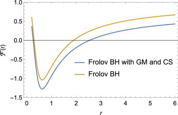
Figure 1. Lapse function ${ \mathcal F }(r)$ as a function of r. It shows that the BH has two horizons. Here, we use a = 0.2, α = 0.2, η = 0.2 and q = 0.6. |
The horizons can be determined using the following condition:
$\begin{eqnarray}1-a-8\,\pi \,{\eta }^{2}-\frac{(2\,Mr-{q}^{2}){r}^{2}}{{r}^{4}+(2\,Mr+{q}^{2}){\alpha }^{2}}=0.\end{eqnarray}$
Unlike the standard RN BH, where horizons can be determined analytically, equation (18 ) has no closed-form solution due to the complex interplay of the Frolov parameter α with the topological defect parameters a and η. The presence of the length scale parameter α fundamentally alters the causal structure of the spacetime, ensuring its regularity at the origin while preserving the horizon structure characteristic of charged BHs.
We employ numerical methods to calculate the event and Cauchy horizons. Tables 1 and 2 present the numerical results for these two horizons under various parameter combinations. Figure 2 depicts the inner horizon and shows how the parameters α, q, a and η influence it, while figure 3 shows the corresponding effects on the outer horizon.
Table 1. Numerical results for the inner and outer horizons of Frolov BH with GM and CS for various values of parameters α and q. Here, a = 0.4 and η = 0.4. |
| q = 0.2 | 0.4 | 0.6 | |||||||
|---|---|---|---|---|---|---|---|---|---|
| α | rh− | rh+ | rh+ − rh− | rh− | rh+ | rh+ − rh− | rh− | rh+ | rh+ − rh− |
| 0.2 | 0.154185 | 4.52142 | 4.36724 | 0.20719 | 4.45982 | 4.25263 | 0.295159 | 4.3531 | 4.05794 |
| 0.4 | 0.294424 | 4.50949 | 4.21507 | 0.352427 | 4.44722 | 4.09479 | 0.445525 | 4.3392 | 3.89368 |
| 0.6 | 0.439386 | 4.48932 | 4.04993 | 0.501542 | 4.42587 | 3.92433 | 0.60167 | 4.3156 | 3.71393 |
Table 2. Numerical results for the inner and outer horizons of the Frolov BH with GM and CS for various values of parameters a and η. Here, α = 0.4 and q = 0.6. |
| η = 0.2 | 0.4 | 0.6 | |||||||
|---|---|---|---|---|---|---|---|---|---|
| a | rh− | rh+ | rh+ − rh− | rh− | rh+ | rh+ − rh− | rh− | rh+ | rh+ − rh− |
| 0.2 | 0.582236 | 2.37048 | 1.78824 | 0.52899 | 2.88963 | 2.36064 | 0.445525 | 4.3392 | 3.89368 |
| 0.4 | 0.495324 | 3.34944 | 2.85412 | 0.445525 | 4.3392 | 3.89368 | 0.357059 | 8.14422 | 7.78716 |
| 0.6 | 0.411624 | 5.35737 | 4.94575 | 0.357059 | 8.14422 | 7.78716 | 0.230508 | 49.8192 | 49.5887 |
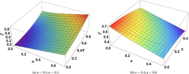
Figure 2. Variation of the inner horizon for different values of α and q in panel (a), and η and a in panel (b). |
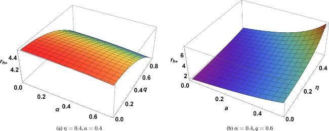
Figure 3. Variation of the outer horizon for different values of α and q in panel (a), and η and a in panel (b). |
Analysis of these figures reveals several important patterns. Figure 2 indicates that α and q have similar effects, with the inner horizon increasing with both (see left panel). However, the inner horizon shrinks substantially when a and η rise (see right panel). Conversely, figure 3 shows that increasing α and q values decrease the outer horizon radius (left panel), while the outer horizon expands significantly as a and η increase (right panel). This opposing behavior between inner and outer horizons under parameter variation illustrates the complex interplay between regularization and topological effects in determining the causal structure of the spacetime.
3. Dynamics of photons in Frolov BH with GM and CS
In this section, we study motions of photon light around the Frolov BH solution with GM and CS and analyze how various parameters, such as the GM and CS parameters and electric charge alter the dynamics of photon light. The geodesic motion of photons provides useful information about the photon sphere radius, BH shadow, and the stability of circular orbits under the influence of a BH's gravitational field. Geodesics motions in various singular and regular BHs have been widely studied in the literature (see, for example, [45–52] and related references therein). The effective potential for null geodesics around a BH is a tool to describe the behavior of light in curved spacetime near a BH. It helps us to understand the motion of light around BHs, particularly in regions where the spacetime is highly curved, such as near the event horizon. The effective potential provides insight into whether photons will be able to escape from the BH’s gravitational pull (if they are outside the photon sphere) or whether they will be captured by the BH. With the help of the effective potential, one can determine the photon sphere radius including the BH shadow and others.
The motion of photon light is described by ds2 = 0. For the given spacetime (13 ), we obtain:
$\begin{eqnarray}\begin{array}{l}-{ \mathcal F }(r)\,{\left(\frac{{\rm{d}}t}{{\rm{d}}\tau }\right)}^{2}+\frac{1}{{ \mathcal F }(r)}\,{\left(\frac{{\rm{d}}r}{{\rm{d}}\tau }\right)}^{2}\\ \,+\,{r}^{2}\,{\left(\frac{{\rm{d}}\theta }{{\rm{d}}\tau }\right)}^{2}+{r}^{2}\,{\sin }^{2}\theta \,{\left(\frac{{\rm{d}}\phi }{{\rm{d}}\tau }\right)}^{2}=0,\end{array}\end{eqnarray}$
where τ represents an affine parameter.Considering the geodesic motion in the equatorial plane defined by θ = π/2 and $\frac{{\rm{d}}\theta }{{\rm{d}}\tau }=0$, we find the following conserved quantities:
$\begin{eqnarray}E={ \mathcal F }(r)\,\left(\frac{{\rm{d}}t}{{\rm{d}}\tau }\right),\quad \quad L={r}^{2}\,\frac{{\rm{d}}\phi }{{\rm{d}}\tau },\end{eqnarray}$
where E is the conserved energy associated with the temporal coordinate and L is the conserved angular momentum.With these, we can rewrite equation (19 ) after rearranging as,
$\begin{eqnarray}{\left(\displaystyle \frac{{\rm{d}}r}{{\rm{d}}\tau }\right)}^{2}+{V}_{\,\rm{eff}\,}(r)={E}^{2},\end{eqnarray}$
which is equivalent to the 1D equation of motion with Veff(r), which is the effective potential given by, $\begin{eqnarray}\begin{array}{rcl}{V}_{\,\rm{eff}\,}(r) & = & \frac{{{L}}^{2}}{{r}^{2}}\,{ \mathcal F }(r)\\ & = & \frac{{{L}}^{2}}{{r}^{2}}\left(1-a-8\,\pi \,{\eta }^{2}-\frac{(2\,M\,r-{q}^{2})\,{r}^{2}}{{r}^{4}+(2\,M\,r+{q}^{2})\,{\alpha }^{2}}\right).\end{array}\end{eqnarray}$
From the expression given in equation (22 ), it is clear that the effective potential for null geodesics is influenced by several factors. These include the energy scale of the symmetry-breaking η, the CS parameter a, the length scale parameter α and the electric charge q. In addition, the conserved angular momentum L and BH mass M alter the effective potential.
In figure 4, we generate a plot showing the effective potential for null geodesics by varying the values of the CS parameter a, the symmetry-breaking energy scale parameter η, and the length scale parameter α, all individually and in combination. In panel (a), we observe that increasing the length scale parameter from α = 0.5 leads to a corresponding rise in the effective potential with increasing the radial coordinate r. In contrast, panels (b) to (f) show that increasing the CS parameter a, the energy scale parameter η, or their combinations with the length scale parameter α, results in a decrease in the effective potential as r increases. Throughout this figure, we fix the BH mass M = 1, the angular momentum L = 1 and the electric charge to q = 0.5. These parameters collectively influence the shape and behavior of the effective potential for null geodesics in the vicinity of the considered BH.
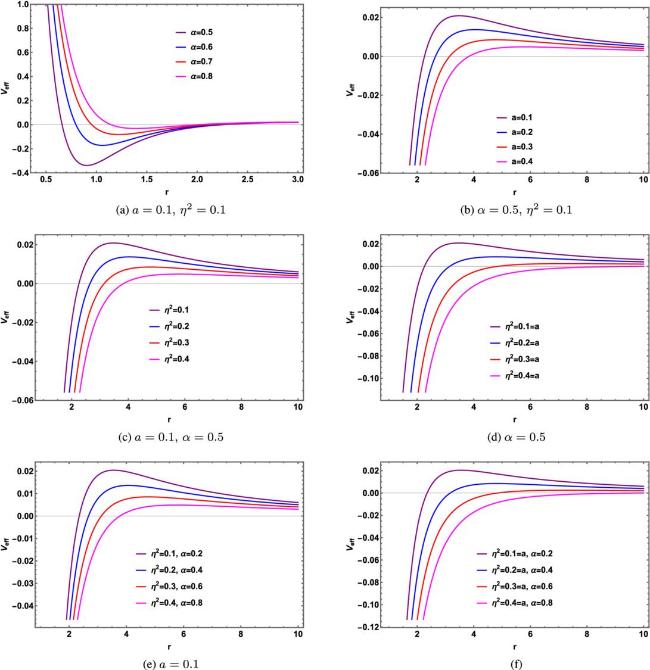
Figure 4. Behavior of the effective potential for null geodesics varying different parameters a, η and α. Here, we set M = 1, L = 1 and q = 0.5. |
In the limit where α = 0, corresponding to the absence of the Frolov parameter, and η = 0, indicating the absence of the symmetry-breaking energy scale, the effective potential given by equation (22 ) reduces to the following: 22 ) reduces to the following:
$\begin{eqnarray}{V}_{\,\rm{eff}\,}(r)=\frac{{{L}}^{2}}{{r}^{2}}\,\left(1-a-\frac{2\,M}{r}+\frac{{q}^{2}}{{r}^{2}}\right).\end{eqnarray}$
Moreover, in the limit where α = 0, corresponding to the absence of the Frolov parameter, and a = 0, indicating the absence of the CS, the effective potential given by equation ( $\begin{eqnarray}{V}_{\,\rm{eff}\,}(r)=\frac{{{L}}^{2}}{{r}^{2}}\,\left(1-8\,\pi \,{\eta }^{2}-\frac{2\,M}{r}+\frac{{q}^{2}}{{r}^{2}}\right).\end{eqnarray}$
Now, we determine the force on photons under the gravitational field produced by the BH and show how various parameters affect the motion of light in the vicinity of the BH. Using the effective potential for null geodesics given in equation (22 ), we can determine the force on photons as,
$\begin{eqnarray}\begin{array}{rcl}{F}_{\,\rm{ph}\,} & = & -\frac{1}{2}\,\frac{{\rm{d}}{V}_{\,\rm{eff}\,}}{{\rm{d}}r}\\ & = & \frac{{{L}}^{2}}{{r}^{3}}\,\left[1-a-8\,\pi \,{\eta }^{2}+\frac{M\,{r}^{3}}{{r}^{4}+(2\,M\,r+{q}^{2})\,{\alpha }^{2}}\right.\\ & & \left.+\frac{(M\,{\alpha }^{2}\,{q}^{2}-2\,{\alpha }^{2}\,{M}^{2}\,r+2\,{q}^{2}\,{r}^{3}-4\,M\,{r}^{4})\,{r}^{3}}{{[{r}^{4}+(2\,M\,r+{q}^{2})\,{\alpha }^{2}]}^{2}}\right].\end{array}\end{eqnarray}$
From the expression given in equation (25 ), it is clear that the force on photon particles depends on various factors. These include the energy scale of the symmetry-breaking η, the CS parameter a, the length scale parameter α and the electric charge q. In addition, the conserved angular momentum L, and BH mass M also alter the force acting on photon particles under the gravitational field produced by the selected charged BH.
In figure 5, we illustrate the behavior of the force acting on photon particles by varying the CS parameter a, the symmetry-breaking energy scale parameter η, and the length scale parameter α, both individually and in combination. In panel (a), we observe that increasing the length scale parameter from α = 0.5 leads to a corresponding increase in the force with the radial coordinate r. This suggests that larger values of α enhance the gravitational field, resulting in a stronger attraction of photon particles. In contrast, panels (b) to (f) show that increasing the CS parameter a, the energy scale parameter η, or their combinations with α, leads to a decrease in the force as r increases. This indicates that larger values of these parameters weaken the effective gravitational field generated by the charged BH, thereby reducing the attraction experienced by photon particles. Throughout the analysis, we fix the BH mass to M = 1, the angular momentum to L = 1 and the electric charge to q = 0.5. Together, these parameters govern the dynamics of photon particles, influencing whether they are captured by or escape from the gravitational field of the BH.
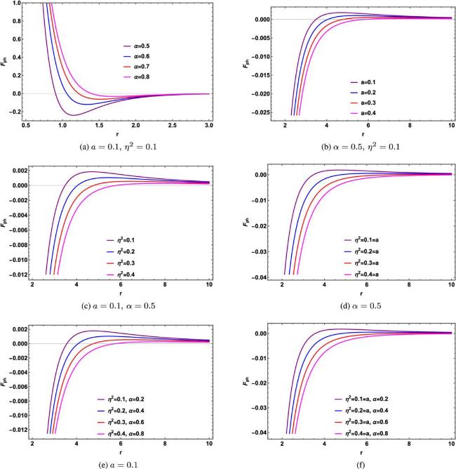
Figure 5. Behavior of force on photon particles by varying different parameters a, η and α. Here, we set M = 1, L = 1 and q = 0.5. |
To differentiate force from the known result, we consider the limit where α = 0, that is the absence of the length scalar parameter in the selected BH solution, zero CS parameter a = 0 and zero the energy scale parameter η = 0. In this limit, the chosen BH solution reduces to RN metric, where the metric function reduces to ${ \mathcal F }\to f=1-\frac{2\,M}{r}+\frac{{q}^{2}}{{r}^{2}}$.
Therefore, the expression of force on photon particles in this limit from equation (25 ) becomes,
$\begin{eqnarray}{F}_{\,\rm{ph}\,}=\frac{{{L}}^{2}}{{r}^{3}}\,\left(1-\frac{3\,M}{r}+\frac{2\,{q}^{2}}{{r}^{2}}\right).\end{eqnarray}$
Thus, comparing the expression of force given in equation (25 ) with that of equation (26 ), it is clear that the current result is modified (either increased or decreased) by the energy scale of the symmetry-breaking η, the CS parameter a and length scale parameter α.
For circular motions around the BH vicinity, we have the conditions $\frac{{\rm{d}}r}{{\rm{d}}\tau }=0$ and $\frac{{{\rm{d}}}^{2}r}{{\rm{d}}{\tau }^{2}}=0$ at radius r = rc yielding the following relations:
$\begin{eqnarray}\begin{array}{rcl}{E}^{2} & = & {V}_{\,\rm{eff}\,}(r)\\ & = & \frac{{{L}}^{2}}{{r}^{2}}\left(1-a-8\,\pi \,{\eta }^{2}-\frac{(2\,M\,r-{q}^{2})\,{r}^{2}}{{r}^{4}+(2\,M\,r+{q}^{2})\,{\alpha }^{2}}\right).\end{array}\end{eqnarray}$
The above relation gives us the critical impact parameter for photon light given by, $\begin{eqnarray}\frac{1}{{\beta }_{c}^{2}}=\frac{{{\rm{E}}}_{\,\rm{ph}\,}}{{{L}}_{\,\rm{ph}\,}}=\frac{1-a-8\,\pi \,{\eta }^{2}}{{r}_{c}^{2}}-\frac{(2\,M\,{r}_{c}-{q}^{2})}{{r}_{c}^{4}+(2\,M\,{r}_{c}+{q}^{2})\,{\alpha }^{2}}.\end{eqnarray}$
From the expression given in equation (28 ), it is clear that the critical impact parameter for photon particles is influenced by several factors. These include the energy scale of the symmetry-breaking η, the CS parameter a, the length scale parameter α and the electric charge q. In addition, the BH mass M alters this impact parameter.
And the second relation is ${V}_{\,\rm{eff}\,}^{{\prime} }(r)=0$ which gives us the photon sphere radius r = rph satisfying the following relation:
$\begin{eqnarray}\begin{array}{l}r\,{{ \mathcal F }}^{{\prime} }(r)-2\,{ \mathcal F }(r)=0\\ \Rightarrow \,1-a-8\,\pi \,{\eta }^{2}+\frac{M\,{r}^{3}}{{r}^{4}+(2\,M\,r+{q}^{2})\,{\alpha }^{2}}\\ +\,\frac{(M\,{\alpha }^{2}\,{q}^{2}-2\,{\alpha }^{2}\,{M}^{2}\,r+2\,{q}^{2}\,{r}^{3}-4\,M\,{r}^{4})\,{r}^{3}}{{[{r}^{4}+(2\,M\,r+{q}^{2})\,{\alpha }^{2}]}^{2}}=0.\end{array}\end{eqnarray}$
We now proceed to analyze how various parameters, such as the GM, CS and electric charge, which are embedded in the spacetime geometry of the Frolov BH, affect the trajectory of photons. The orbital equation using equations (20 ) and (21 ) is obtained as follows:
$\begin{eqnarray}\displaystyle \begin{array}{l}{\left(\frac{{\rm{d}}r}{{\rm{d}}\phi }\right)}^{2}=\frac{{\dot{r}}^{2}}{{\dot{\phi }}^{2}}\\ =\,{r}^{4}\,\left[\frac{1}{{\beta }^{2}}-\frac{1}{{r}^{2}}\,\left(1-a-8\,\pi \,{\eta }^{2}-\frac{(2\,M\,r-{q}^{2})\,{r}^{2}}{{r}^{4}+(2\,M\,r+{q}^{2})\,{\alpha }^{2}}\right)\right],\end{array}\end{eqnarray}$
where β = L/E is the impact parameter for photons.Transforming to a new variable via $r=\frac{1}{u}$, where $\frac{{\rm{d}}r}{{\rm{d}}\phi }=-\frac{1}{{u}^{2}}\,\frac{{\rm{d}}u}{{\rm{d}}\phi }$. The equation of orbit (30 ) can be re-written as follows: 31 ) w. r. t. φ and after simplification, we find:32 ) represents a second-order differential equation that governs the motion of photon trajectories in the modified Frolov BH spacetime, incorporating the combined effects of two topological defects, the GM and CS.
$\begin{eqnarray}\begin{array}{l}{\left(\frac{{\rm{d}}u}{{\rm{d}}\phi }\right)}^{2}+\left(1-a-8\,\pi \,{\eta }^{2}\right)\,{u}^{2}\\ \,=\,\frac{1}{{\beta }^{2}}+\frac{(2\,M-{q}^{2}\,u)\,{u}^{3}}{1+(2\,M+{q}^{2}\,u)\,{\alpha }^{2}\,{u}^{3}}.\end{array}\end{eqnarray}$
Differentiating both sides of equation ( $\begin{eqnarray}\begin{array}{l}\frac{{{\rm{d}}}^{2}u}{{\rm{d}}{\phi }^{2}}+\left(1-a-8\,\pi \,{\eta }^{2}\right)\,u\\ \,=\,\frac{3\,M\,{u}^{2}-2\,{q}^{2}\,{u}^{3}+2\,M\,{q}^{2}\,{\alpha }^{2}\,{u}^{6}}{{\left(1+2M{\alpha }^{2}{u}^{3}+{q}^{2}{\alpha }^{2}{u}^{4}\right)}^{2}}.\end{array}\end{eqnarray}$
Equation (In the limit where α = 0 corresponds to the absence of the Frolov parameter, the photon trajectories from equation (32 ) reduce as,33 ) represents a second-order differential equation governing photon trajectories in the RN BH, incorporating the effects of dual topological defects, the GM and CS.
$\begin{eqnarray}\frac{{{\rm{d}}}^{2}u}{{\rm{d}}{\phi }^{2}}+(1-a-8\,\pi \,{\eta }^{2})\,u=3\,M\,{u}^{2}-2\,{q}^{2}\,{u}^{3}.\end{eqnarray}$
Equation (In the limit where α = 0, corresponding to the absence of the Frolov parameter, and η = 0, indicating the absence of the symmetry-breaking energy scale, the photon trajectory given by equation (32 ) reduces to the following: 34 ) represents a second-order differential equation governing photon trajectories in the RN BH surrounded by a CS. This equation further reduces to the case of the Letelier BH in the limit q → 0.
$\begin{eqnarray}\frac{{{\rm{d}}}^{2}u}{{\rm{d}}{\phi }^{2}}+(1-a)\,u=3\,M\,{u}^{2}-2\,{q}^{2}\,{u}^{3}.\end{eqnarray}$
Equation (In the limit where α = 0, corresponding to the absence of the Frolov parameter, and a = 0, indicating the absence of the CS, the photon trajectory given by equation (32 ) reduces to the following: 34 ) represents a second-order differential equation governing photon trajectories in the RN BH with a GM. This equation further reduces to the case of a GM spacetime in the limit q → 0.
$\begin{eqnarray}\frac{{{\rm{d}}}^{2}u}{{\rm{d}}{\phi }^{2}}+(1-8\,\pi \,{\eta }^{2})\,u=3\,M\,{u}^{2}-2\,{q}^{2}\,{u}^{3}.\end{eqnarray}$
Equation (Now, the radial equation along the time coordinate using equations (20 ) and (21 ) is described by the following equation: 20 ), (21 ), (31 ) and (36 ).
$\begin{eqnarray}{\left(\frac{{\rm{d}}r}{{\rm{d}}t}\right)}^{2}=\frac{{\dot{r}}^{2}}{{\dot{t}}^{2}}={{ \mathcal F }}^{2}(r)\,\left(1-\frac{{\beta }^{2}}{{r}^{2}}\,{ \mathcal F }(r)\right).\end{eqnarray}$
Thus, photon motion in the selected Frolov BH with GM and CS is completely described by the equations (For radial photon motion, characterized by a trajectory with vanishing angular momentum (L = 0), photons may either escape away from the singularity or inevitably fall into it. From equations (20 ), (21 ) and (36 ), we obtain: 14 ).
$\begin{eqnarray}\frac{{\rm{d}}t}{{\rm{d}}\tau }=\frac{E}{{ \mathcal F }(r)},\quad \frac{{\rm{d}}r}{{\rm{d}}\tau }=\pm \,E.\end{eqnarray}$
And $\begin{eqnarray}\begin{array}{rcl}\frac{{\rm{d}}r}{{\rm{d}}t} & = & \pm \,{ \mathcal F }(r)\\ & = & \pm \left(1-a-8\,\pi \,{\eta }^{2}-\frac{(2\,Mr-{q}^{2}){r}^{2}}{{r}^{4}+(2\,Mr+{q}^{2}){\alpha }^{2}}\right),\end{array}\end{eqnarray}$
where the sign +(−) corresponds to photons moving towards spatial infinity (are getting closer to the event horizon). Here, ${ \mathcal F }(r)$ is the metric function given in equation (From the expressions given in equations (31 ) and (38 ), it is clear that the photon trajectories for angular motion (L ≠ 0) and radial motion (L = 0) are influenced by several parameters. These include the energy scale of the symmetry-breaking parameter η, the CS parameter a, the length scale parameter α, the electric charge q and the BH mass M.
For radial photon motion, assuming that photons are placed at r = ri when t = τ = 0 and then they approach to r+. A straightforward integration of equation (37 ) yields the following:
$\begin{eqnarray}r(\tau )={r}_{i}-E\,\tau ,\end{eqnarray}$
which then takes an affine parameter τ+ = (ri − r+)/E to reach the event horizon.We now turn our attention to an important physical quantity that determines the stability of circular null orbits, the Lyapunov exponent. This exponent characterizes the (in)stability of the orbits and is derived from the second derivative of the effective potential for null geodesics, as follows [53]:20 ).
$\begin{eqnarray}{\lambda }_{{\rm{L}}}^{\rm{null}\,}=\sqrt{-\frac{{V}_{\,\rm{eff}}^{{\prime\prime} }(r)}{2\,{\dot{t}}^{2}}},\end{eqnarray}$
where $\dot{t}$ is given in equation (Using the effective potential for null geodesics given in equation (22 ), we find the Lyapunov exponent for circular null geodesics in terms of the metric function ${ \mathcal F }(r)$ as follows:
$\begin{eqnarray}{\lambda }_{{\rm{L}}}^{\,\rm{null}\,}=\sqrt{{ \mathcal F }(r)\,\left(\frac{{ \mathcal F }}{{r}^{2}}-\frac{{{ \mathcal F }}^{{\prime\prime} }}{2}\right)}{\left|\right.}_{r={r}_{c}},\end{eqnarray}$
where we have used the relation $r\,{{ \mathcal F }}^{{\prime} }(r)=2\,{ \mathcal F }(r)$.Substituting the metric function given in equation (14 ), we find the Lyapunov exponent for circular null orbits as (setting 8 π = 1):
$\begin{eqnarray}\begin{array}{rcl}{\lambda }_{{\rm{L}}}^{\,\rm{null}\,} & = & \left[-\frac{\left(1-a-8\,\pi \,{\eta }^{2}-\frac{(2\,M\,r-{q}^{2})\,{r}^{2}}{{r}^{4}+(2\,M\,r+{q}^{2})\,{\alpha }^{2}}\right)}{{r}^{2}\,{\left({r}^{4}+({q}^{2}+2\,M\,r)\,{\alpha }^{2}\right)}^{3}}\right.\\ & & \times \left\{{q}^{6}\,{\alpha }^{6}\,(-1+a+{\eta }^{2})+{q}^{4}\,r\,{\alpha }^{2}\right.\\ & & \times \left(-14\,{r}^{5}-8\,M\,{r}^{2}\,{\alpha }^{2}+3\,{r}^{3}\,{\alpha }^{2}\,(-1+a+{\eta }^{2})\right.\\ & & \left.+6\,M\,{\alpha }^{4}\,(-1+a+{\eta }^{2})\right)+{q}^{2}\,{r}^{2}\\ & & \times \left(2\,{r}^{8}+12\,M\,{r}^{5}\,{\alpha }^{2}-8\,{M}^{2}\,{r}^{2}\,{\alpha }^{4}+3\,{r}^{6}\,{\alpha }^{2}\,\right.\\ & & \times (-1+a+{\eta }^{2})+12\,M\,{r}^{3}\,{\alpha }^{4}\,(-1+a+{\eta }^{2})\\ & & \left.+12\,{M}^{2}\,{\alpha }^{6}\,(-1+a+{\eta }^{2})\right)+{r}^{3}\,\left(36\,{M}^{2}\,{r}^{5}\,{\alpha }^{2}\right.\\ & & +{r}^{9}\,(-1+a+{\eta }^{2})+6\,M\,{r}^{6}\,{\alpha }^{2}\,(-1+a+{\eta }^{2})\\ & & +12\,{M}^{2}\,{r}^{3}\,{\alpha }^{4}\,(-1+a+{\eta }^{2})\\ & & {\left.{\left.\left.\left.+8\,{M}^{3}\,{\alpha }^{6}\,(-1+a+{\eta }^{2})\right)\right\}\Space{0ex}{4.98ex}{0ex}\right]}^{1/2},\Space{0ex}{4.5ex}{0ex}\right|}_{r={r}_{c}}.\end{array}\end{eqnarray}$
In figure 6, we present the behavior of the square of the Lyapunov exponent associated with circular null geodesics by varying the CS parameter a, the symmetry-breaking energy scale parameter η, and the length scale parameter α, both individually and in combination. In panel (a), we observe that increasing the length scale parameter from α = 0.5 results in positive values of the Lyapunov exponent squared as a function of the radial coordinate r. This indicates that larger values of α enhance the gravitational field, leading to exponential divergence or convergence of nearby circular null trajectories, signifying chaotic behavior and unstable circular orbits. In contrast, panels (b) to (f) show that increasing the CS parameter a, the energy scale η, or their combinations with α, causes fluctuations in the square of the Lyapunov exponent with respect to r. This behavior suggests that larger values of these parameters reduce the effective gravitational strength of the charged BH, leading to regions where circular orbits may alternate between stability and instability, depending on the radial distance r = rc, where rc is the radius of the circular null orbits. Throughout the analysis, we fix the BH mass to M = 1, the angular momentum to L = 1 and the electric charge to q = 0.5.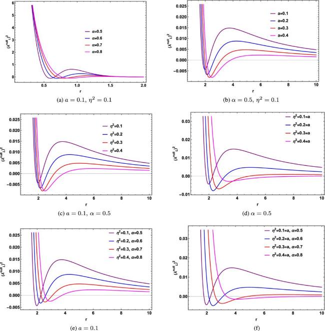
Figure 6. Behavior of the square of the Lyapunov exponent by varying different parameters a, η and α. Here, we set M = 1, L = 1 and q = 0.5. |
In the limit where α = 0, corresponding to the absence of the Frolov parameter, and η = 0, indicating the absence of the symmetry-breaking energy scale, the Lyapunov exponent from equation (42 ) reduces as, 42 ) reduces as, 43 ) and (44 ) represent the Lyapunov exponent expression for circular null orbits in a charged BH surrounded by a CS and a charged BH with a GM, respectively.
$\begin{eqnarray}{\lambda }_{{\rm{L}}}^{\,\rm{null}\,}\,=\,\frac{1}{r}{\left.\sqrt{\left(1-a-\frac{2\,M}{r}+\frac{{q}^{2}}{{r}^{2}}\right)\,\left(1-a-\frac{2\,{q}^{2}}{{r}^{2}}\right)}\right|}_{r={r}_{c}}.\end{eqnarray}$
Moreover, in the limit where α = 0, corresponding to the absence of the Frolov parameter, and a = 0, indicating the absence of the CS effects, the Lyapunov exponent from equation ( $\begin{eqnarray}\begin{array}{l}{\lambda }_{{\rm{L}}}^{\,\rm{null}\,}\\ \,=\frac{1}{r}{\left.\sqrt{\left(1-8\,\pi \,{\eta }^{2}-\frac{2\,M}{r}+\frac{{q}^{2}}{{r}^{2}}\right)\,\left(1-8\,\pi \,{\eta }^{2}-\frac{2\,{q}^{2}}{{r}^{2}}\right)}\right|}_{r={r}_{c}}.\end{array}\end{eqnarray}$
Equations (The geodesics angular velocity (called coordinate velocity) is defined by [53],
$\begin{eqnarray}\omega =\frac{\dot{\phi }}{\dot{t}}=\frac{\sqrt{{ \mathcal F }(r)}}{r}.\end{eqnarray}$
Here, we have used the relation $E=\frac{{L}}{r}\,\sqrt{{ \mathcal F }}$.Substituting the metric function given in equation (14 ), we find the geodesic angular velocity:
$\begin{eqnarray}\omega =\sqrt{\frac{1-a-8\,\pi \,{\eta }^{2}}{{r}^{2}}-\frac{(2\,M\,r-{q}^{2})}{{r}^{4}+(2\,M\,r+{q}^{2})\,{\alpha }^{2}}}.\end{eqnarray}$
From the expression given in equation (46 ), it is clear that null geodesics angular velocity in the equatorial plane depend on various factors. These include the energy scale of the symmetry-breaking η, the CS parameter a and the length scale parameter α. In addition, the BH mass M and charge q also alter the angular velocity under the given gravitational field of the charged BH.
In the limit where α = 0, corresponding to the absence of the Frolov parameter, and η = 0, indicating the absence of the symmetry-breaking energy scale, the angular velocity from equation (46 ) reduces as, 42 ) reduces as, 47 ) and (48 ) represent the geodesic angular velocities for a charged BH surrounded by a CS and a charged BH with a GM, respectively.
$\begin{eqnarray}\omega =\frac{1}{r}\sqrt{1-a-\frac{2\,M}{r}+\frac{{q}^{2}}{{r}^{2}}}.\end{eqnarray}$
Moreover, in the limit where α = 0, corresponding to the absence of the Frolov parameter, and a = 0, indicating the absence of the CS effects, the angular velocity from equation ( $\begin{eqnarray}\omega =\frac{1}{r}\sqrt{1-8\,\pi \,{\eta }^{2}-\frac{2\,M}{r}+\frac{{q}^{2}}{{r}^{2}}}.\end{eqnarray}$
Equations (4. Thermodynamics of the Frolov BH with GM and CS
The thermodynamic analysis of BHs has become a cornerstone in understanding the deep connections between gravity, quantum theory and information science [22, 23]. For modified BH solutions, such as the Frolov BH with GM and CS, examining thermodynamic properties reveals distinctive behaviors that differentiate these solutions from classical BHs and potentially lead to observable signatures [54]. In this section, we conduct a comprehensive thermodynamic analysis of the Frolov BH with GM and CS, investigating how the interplay between the length scale parameter α, charge q, GM parameter η and CS parameter a influences various thermodynamic quantities.
Let us begin by deriving the mass function for the Frolov BH with GM and CS. By applying the horizon condition ${ \mathcal F }({r}_{+})=0$ at the event horizon radius r+, we obtain:
$\begin{eqnarray}{M}_{H}=\frac{{q}^{2}({r}_{+}^{2}-{\alpha }^{2}(a+{\eta }^{2}-1))-{r}_{+}^{4}(a+{\eta }^{2}-1)}{2{r}_{+}^{2}({r}_{+}^{2}-{\alpha }^{2}+a{\alpha }^{2}+{\alpha }^{2}{\eta }^{2})}.\end{eqnarray}$
The mass function in equation (49 ) differs significantly from that of standard BH solutions due to the complex interplay between the Frolov parameter α and the topological defect parameters a and η [55]. Unlike the Arnowitt, Deser and Misner (ADM) mass in asymptotically flat spacetimes, the mass MH here incorporates the contribution of the background geometry modified by the GM and CS. In specific limits, we recover known results. Without GM and CS (a = 0 = η), equation (49 ) reduces to the mass of the original Frolov BH [55], and when α = 0, it reduces to the mass of the RN BH as ${M}_{H}=\frac{{q}^{2}+{r}_{+}^{2}}{2{r}_{+}}$.
Figure 7 illustrates how the BH parameters impact the mass function. The mass exhibits characteristic behavior. It initially decreases exponentially, reaching a minimum at a critical horizon radius, after which it increases monotonically with increasing horizon radius. This behavior is consistent with both the original Frolov BH and the RN BH. Our analysis focuses primarily on the parameters α and a since the behavior of q and η is comparable to that of α and a, respectively.
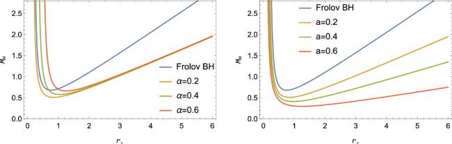
Figure 7. Mass of the Frolov BH with GM and CS showing the influence of the length scale parameter (left) and the CS parameter (right). Here, q = 0.6 and η = 0.4. |
Next, we determine the Hawking temperature based on the relationship between surface gravity and metric components in the semi-classical framework [56]. The temperature of a BH is proportional to its surface gravity κ at the event horizon through the relation T = κ/2π [57]. For the Frolov BH with GM and CS, the Hawking temperature takes the following form:
$\begin{eqnarray}{T}_{+}=\frac{{q}^{2}(4{r}_{+}^{2}{\alpha }^{2}(a+{\eta }^{2}-1)-{r}_{+}^{4})-{r}_{+}^{4}(a+{\eta }^{2}-1)(3{\alpha }^{2}(a+{\eta }^{2}-1)+{r}_{+}^{2})+{\alpha }^{2}{(a+{\eta }^{2}-1)}^{2}}{4\pi \,{r}_{+}^{3}({r}_{+}^{4}+{q}^{2}{\alpha }^{2})}.\end{eqnarray}$
The temperature expression in equation (50 ) reveals how the thermodynamic behavior of the BH is influenced by the combined effects of the Frolov parameter and topological defects [58]. This modification has significant implications for the BH’s evaporation process and final state, potentially avoiding the complete evaporation predicted for classical BHs [59]. In specific limits, we recover known results. Without GM and CS (a = 0 = η), equation (50 ) reduces to the temperature of the original Frolov BH [55], and when α = 0, it reduces to the temperature of the RN BH as ${T}_{+}=\frac{{r}_{+}^{2}-{q}^{2}}{4\pi {r}_{+}^{3}}$.
Figure 8 illustrates how the Hawking temperature T+ varies with the horizon radius and model parameters. The temperature initially rises with increasing horizon radius, reaches a peak, and then falls as the horizon radius increases further. The peak temperature decreases as α increases (with a, η and q held constant), and also decreases with increasing charge q. This behavior is consistent with both the original Frolov BH and the RN BH. As with the mass analysis, we focus primarily on the parameters α and a since q and η exhibit behaviors similar to those of α and a, respectively.
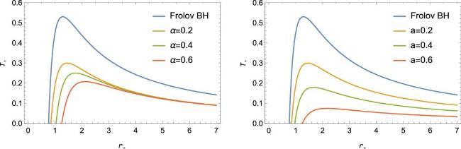
Figure 8. Temperature of the Frolov BH with GM and CS showing the influence of the length scale parameter (left) and the CS parameter (right). Here, q = 0.6 and η = 0.4. |
In the limit where α = 0, corresponding to the absence of the Frolov parameter, and η = 0, indicating the absence of the symmetry-breaking energy scale, the Hawking temperature from equation (50 ) reduces as, 42 ) reduces as, 50 ) and (52 ) represent the Hawking temperature for a charged BH surrounded by a CS and a charged BH with a GM, respectively.
$\begin{eqnarray}{T}_{+}=\frac{1}{4\,\pi \,{r}_{+}}\,\left(1-a-\frac{{q}^{2}}{{r}_{+}^{2}}\right).\end{eqnarray}$
Moreover, in the limit where α = 0, corresponding to the absence of the Frolov parameter, and a = 0, indicating the absence of the CS effects, the Hawking temperature from equation ( $\begin{eqnarray}{T}_{+}=\frac{1}{4\,\pi \,{r}_{+}}\,\left(1-8\,\pi \,{\eta }^{2}-\frac{{q}^{2}}{{r}_{+}^{2}}\right).\end{eqnarray}$
Equations (To determine the entropy of the BH, we apply the first law of thermodynamics (dM = T+dS+ + Φ dq), which yields: 53 ) deviates significantly from the Bekenstein–Hawking area law that characterizes standard BH solutions [60]. In classical BH thermodynamics, the entropy is proportional to the area of the event horizon, S = A/4. However, for the Frolov BH with GM and CS, the entropy contains additional terms that reflect the modified causal structure of the spacetime [61]. This deviation has profound implications for information theory and the resolution of the information paradox [62].
$\begin{eqnarray}\begin{array}{rcl}{S}_{+} & = & \displaystyle \int \frac{1}{{T}_{+}}\frac{\partial M}{\partial {r}_{+}}{\rm{d}}{r}_{+}\\ & = & \frac{\pi }{4}\left({r}_{+}^{2}-\frac{{\alpha }^{2}(2{q}^{2}+{\alpha }^{2}{(a+{\eta }^{2}-1)}^{2})}{{r}_{+}^{2}+{\alpha }^{2}(a+{\eta }^{2}-1)}\right.\\ & & \left.-2{\alpha }^{2}\left(a+{\eta }^{2}-1\right)\Space{0ex}{3.5ex}{0ex}\right)\\ & & \times {\mathrm{log}}\,[{r}_{+}^{2}+{\alpha }^{2}(a+{\eta }^{2}-1)].\end{array}\end{eqnarray}$
The entropy expression in equation (To analyze the thermodynamic stability of the system, we calculate the specific heat capacity (C+), which describes how the BH responds to temperature fluctuations. A positive value of specific heat indicates local stability (the system can absorb heat while maintaining a moderate temperature increase), whereas negative values imply local instability (temperature increases as mass decreases). The specific heat is determined using ${C}_{+}=\frac{{\rm{d}}M}{{\rm{d}}{T}_{+}}$, which gives:
$\begin{eqnarray}{C}_{+}=\frac{-2\pi \,{r}_{+}^{4}{({r}_{+}^{4}+2{q}^{2}{\alpha }^{2})}^{2}}{2{q}^{4}{\alpha }^{2}({r}_{+}^{2}+{\alpha }^{2}X)({r}_{+}^{2}+3{\alpha }^{2}X)-{r}_{+}^{8}X({r}_{+}^{2}+9{\alpha }^{2}X)+{q}^{2}{r}_{+}^{4}(-3{r}_{+}^{4}+26{r}_{+}^{2}{\alpha }^{2}X+13{\alpha }^{4}{X}^{2})},\end{eqnarray}$
where X = a + η2 − 1.The heat capacity expression in equation (54 ) reveals the complex thermodynamic structure of the Frolov BH with GM and CS, with multiple phase transitions possible depending on parameter values [63]. The sign changes in the heat capacity indicate transitions between thermodynamically stable and unstable phases, which have significant implications for the BH’s evolutionary path and final state [25]. In specific limits, we recover known results. Without GM and CS (a = 0 = η), equation (54 ) reduces to the heat capacity of the original Frolov BH [55], and when α = 0, it reduces to the specific heat capacity of the RN BH as ${C}_{+}=\frac{2\pi (3{q}^{2}-{r}_{+}^{2})}{{r}_{+}^{4}}$.
Equation (54 ) for heat capacity is intricate and challenging to interpret, hence it is depicted in figures 9 and 10. Figure 9 shows the heat capacity for various values of the length scale parameter α (with fixed values a = 0.2, q = 0.6 and η = 0.4). The heat capacity diverges at two critical radii, r1 and r2, indicating a stable region for r1 < r+ < r2 and an unstable region for r+ > r2. This behavior reveals a phase transition at r2 from a smaller stable BH to a larger unstable BH. Figure 10 shows similar behavior for various values of the CS parameter a (with fixed values α = 0.2, q = 0.6 and η = 0.4).
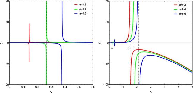
Figure 9. Specific heat capacity of the Frolov BH with GM and CS showing the influence of the length scale parameter for small values of horizon r+ (left) and large values (right). Here, q = 0.6 and η = 0.4. |
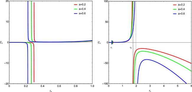
Figure 10. Specific heat capacity of the Frolov BH with GM and CS showing the influence of the CS parameter for small values of horizon r+ (left) and large values (right). Here, q = 0.6 and η = 0.4. |
The phase structure revealed by this heat capacity analysis has important implications for the BH’s evaporation process and final state [64]. The stable region between r1 and r2 suggests that the BH may reach a thermodynamic equilibrium state rather than evaporating completely, potentially resolving some of the paradoxes associated with the final stages of BH evaporation [65]. Furthermore, the influence of the GM and CS parameters on the phase transitions indicates that topological defects can fundamentally alter the thermodynamic behavior of BHs, providing potential observational signatures of such exotic objects [66].
5. Shadow of the Frolov BH with GM and CS
The detection of BH shadows by the Event Horizon Telescope collaboration has opened a new observational window into strong-field gravity, making the theoretical investigation of BH shadows increasingly relevant for testing alternative gravity theories and exotic BH models [3]. The BH shadow represents the apparent image of the photon capture region as seen by a distant observer, effectively marking the boundary between photons that escape to infinity and those captured by the BH [27]. For modified BH solutions, such as the Frolov BH with GM and CS, the shadow characteristics can serve as distinctive observational signatures that potentially distinguish these models from classical GR solutions [30, 31].
The formation of a BH shadow is intimately connected to the existence of a photon sphere, a region where light rays can orbit the BH in unstable circular paths. For spherically symmetric spacetimes, the photon sphere corresponds to the critical radius where the effective potential for null geodesics reaches its maximum [67]. The shadow radius, which determines the apparent size of the BH as seen by a distant observer, is then calculated based on the impact parameter of the critical null geodesics that define the boundary of the shadow [68].
This section examines how model parameters of the Frolov BH with GM and CS affect the shadow radius. Spherically symmetric and static metrics with a photon sphere allow an observer to view an infinite number of images of a light source. We can determine the photon orbit radius using the following relation:
$\begin{eqnarray}{r}_{\,\rm{ph}\,}\,{{ \mathcal F }}^{{\prime} }({r}_{\,\rm{ph}\,})=2\,{ \mathcal F }({r}_{\,\rm{ph}\,}).\end{eqnarray}$
This condition arises from analyzing the geodesic equations for null particles in the Frolov BH with GM and CS spacetime. By considering the Lagrangian for geodesic motion and applying the Euler–Lagrange equations, one obtains equations of motion that govern the trajectory of light rays [69]. The condition for circular photon orbits is derived by setting the radial velocity and acceleration to zero, leading to the characteristic equation above that determines the radius of the photon sphere [70].Considering the metric function in equation (14 ), the equation for rph becomes: 56 ) reduces to the following: 57 ) represents the photon sphere radius in the RN BH coupled with a CS and GM.
$\begin{eqnarray}\begin{array}{l}(1-a-8\,\pi \,{\eta }^{2})-\frac{(2\,M\,{r}_{\,\rm{ph}\,}-{q}^{2})\,{r}_{{\rm{p}}{\rm{h}}}^{2}}{{r}_{{\rm{p}}{\rm{h}}}^{4}+{\alpha }^{2}\,(2\,M\,{r}_{\,\rm{ph}\,}+{q}^{2})}\\ +\frac{{r}_{\,\rm{ph}\,}\,\left[(6\,M\,{r}_{\,\rm{ph}\,}-2\,{q}^{2}\,{r}_{\,\rm{ph}\,})({r}_{\,\rm{ph}\,}^{4}+{\alpha }^{2}\,(2\,M\,{r}_{\,\rm{ph}\,}+{q}^{2}))-(2\,M\,{r}_{\,\rm{ph}\,}^{3}-{q}^{2}\,{r}_{\,\rm{ph}\,}^{2})(4\,{r}_{\,\rm{ph}\,}^{3}+2\,M\,{\alpha }^{2})\right]}{2\,{\left[{r}_{\,\rm{ph}\,}^{4}+{\alpha }^{2}\,(2\,M\,{r}_{\,\rm{ph}\,}+{q}^{2})\right]}^{2}}=0.\end{array}\end{eqnarray}$
In the limit where α = 0, corresponding to the absence of the Frolov parameter, the photon sphere relation given by equation ( $\begin{eqnarray}\begin{array}{l}(1-a-8\,\pi \,{\eta }^{2})\,{r}_{\,\rm{ph}\,}^{2}-3\,M\,{r}_{\,\rm{ph}\,}+2\,{q}^{2}=0\Rightarrow {r}_{\,\rm{ph}\,}\\ \,=\,\frac{3\,M}{2\,(1-a-8\,\pi \,{\eta }^{2})}\\ \,\times \,\left[1+\sqrt{1-\frac{8\,(1-a-8\,\pi \,{\eta }^{2})\,{q}^{2}}{9\,{M}^{2}}}\right].\end{array}\end{eqnarray}$
Equation (Moreover, in the limit where α = 0, corresponding to the absence of the Frolov parameter, and η = 0, indicating the absence of symmetry-breaking energy scale, the photon sphere radius using equation (56 ) becomes: 58 ) represents the photon sphere radius in the RN BH surrounded by a CS only.
$\begin{eqnarray}{r}_{\,\rm{ph}\,}=\frac{3\,M}{2\,(1-a)}\,\left[1+\sqrt{1-\frac{8\,(1-a)\,{q}^{2}}{9\,{M}^{2}}}\right].\end{eqnarray}$
Equation (In addition, in the limit where α = 0, corresponding to the absence of the Frolov parameter, and a = 0, indicating the absence of the CS, the photon sphere relation given by equation (56 ) reduces to the following: 59 ) represents the photon sphere radius in the RN BH with a GM only.
$\begin{eqnarray}{r}_{\,\rm{ph}\,}=\frac{3\,M}{2\,(1-8\,\pi \,{\eta }^{2})}\,\left[1+\sqrt{1-\frac{8\,(1-8\,\pi \,{\eta }^{2})\,{q}^{2}}{9\,{M}^{2}}}\right].\end{eqnarray}$
Equation (The complexity of equation (56 ) reflects the intricate interplay between the Frolov parameter α, the charge q and the topological defect parameters a and η to determine the location of the photon sphere. Unlike the Schwarzschild BH, where the photon sphere occurs at a fixed radius rph = 3M, or the RN BH, where the photon sphere depends only on mass and charge, the Frolov BH with GM and CS exhibits a more complex dependence on multiple parameters [71]. This complexity arises from the modified gravitational potential due to both the regular Frolov core and the topological defects, which alter the effective potential experienced by photons [72].
Since equation (56 ) cannot be solved analytically, we employ numerical techniques to determine the photon orbit radii rph. Once we obtain these values, we calculate the shadow radii using: 60 ) represents the apparent size of the BH as seen by a distant observer in the equatorial plane. Physically, it corresponds to the critical impact parameter that separates the capture and scattering orbits for light rays approaching the BH [73]. For observers at infinity, this critical impact parameter manifests itself as the radius of a dark circular region against a bright background, the BH shadow. Tables 3 and 4 present numerical values of the photon sphere and shadow radii for various combinations of parameters of the Frolov BH with GM and CS. These tabulated results allow for a systematic analysis of how each parameter influences the shadow characteristics, providing quantitative predictions that could potentially be compared with observational data from instruments such as the Event Horizon Telescope [74].
$\begin{eqnarray}{R}_{s}=\frac{{r}_{\,\rm{ph}\,}}{\sqrt{{ \mathcal F }({r}_{\,\rm{ph}\,})}}.\end{eqnarray}$
The shadow radius formula in equation (Table 3. Numerical results for the photon radius and shadow radius with various BH parameters, α and q. Here, a = 0.4 and η = 0.4. |
| q = 0.2 | 0.4 | 0.6 | ||||
|---|---|---|---|---|---|---|
| α | rph | Rs | rph | Rs | rph | Rs |
| 0.2 | 6.78791 | 17.7464 | 6.70612 | 17.5868 | 6.56508 | 17.3127 |
| 0.4 | 6.77736 | 17.7327 | 6.69504 | 17.5724 | 6.55301 | 17.2972 |
| 0.6 | 6.75961 | 17.7096 | 6.67639 | 17.5482 | 6.53265 | 17.2709 |
Table 4. Numerical results for the photon radius and shadow radius with various BH parameters, a and η. Here, α = 0.4 and q = 0.6. |
| η = 0.2 | 0.4 | 0.6 | ||||
|---|---|---|---|---|---|---|
| a | rph | Rs | rph | Rs | rph | Rs |
| 0.2 | 3.63485 | 7.40957 | 4.39661 | 9.70029 | 6.55301 | 17.2972 |
| 0.4 | 5.0779 | 11.9337 | 6.55301 | 17.2972 | 12.2508 | 43.5389 |
| 0.6 | 8.07556 | 23.5079 | 12.2508 | 43.5389 | 74.7591 | 647.955 |
The shadow radius exhibits particular sensitivity to the parameters of the topological defects, as evidenced by the dramatic increase in shadow size with increasing values of a and η in table 4. This enhanced sensitivity could provide a distinctive observational signature for the identification of BHs with topological defects, as the shadow size would appear significantly larger than expected for a classical BH of equivalent mass [28]. Tables 3 and 4 reveal an interesting pattern. Frolov BH parameters (q, α) and topological defect parameters (η, a) affect the shadow radius in opposite ways. Increasing the Frolov parameters (q, α) decreases the shadow radius, while increasing the topological defect parameters (η, a) increases it. Figures 11 and 12 illustrate these opposing tendencies using 3D visualizations and contour plots, providing a comprehensive view of the dependencies of the parameters.
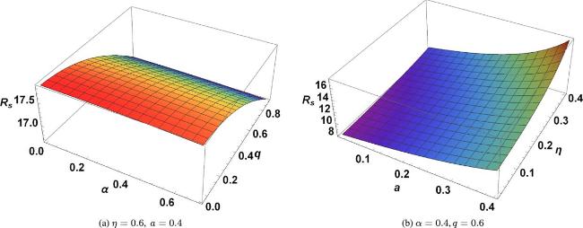
Figure 11. Variation of the shadow radius for different values of α and q (left), and for different values of η and a (right). |
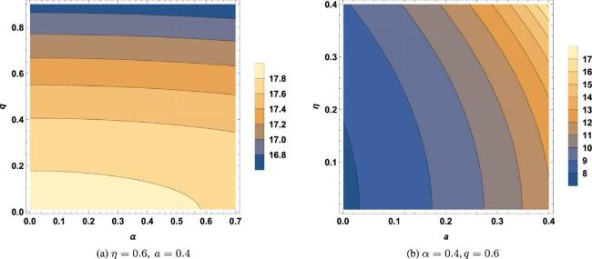
Figure 12. Contour plot of the shadow radius for different values of α and q (left), and for different values of η and a (right). |
These opposing tendencies reveal the complex interplay between the Frolov regularization and topological defects in shaping the causal structure of spacetime. The decrease in shadow radius with increasing Frolov parameters (q, α) stems from the regularization of the central singularity, which modifies the near-horizon geometry and effectively reduces the photon capture cross-section. Conversely, the increase in shadow radius with increasing topological defect parameters (η, a) reflects the additional gravitational effects introduced by the GM and CS, which enhance the light-bending capabilities of the spacetime and consequently enlarge the photon capture region.
The contour plots in figure 12 offer valuable visualizations of these parameter dependencies, showing how the shadow radius varies across the parameter space. These visualizations could guide observational efforts by indicating which parameter regimes would produce the most distinctive shadow characteristics compared to classical BH solutions. The dramatic increase in shadow radius for large values of the topological defect parameters suggests that BHs with significant GM and CS components would exhibit shadows that are substantially larger than their classical counterparts, potentially providing a clear observational signature [75].
From an observational perspective, these results suggest that BHs with GM and CS could be distinguished from classical BHs through precise shadow measurements. Current and future observations by the Event Horizon Telescope collaboration and other facilities could potentially constrain the presence and magnitude of these topological defects in astrophysical BHs by comparing measured shadow sizes with theoretical predictions across the parameter space [76].
6. Scalar and EM perturbations in Frolov BH geometry
Perturbation analysis serves as a powerful tool for probing the stability and spectral characteristics of BH spacetimes. It allows researchers to study how BHs respond to small external disturbances, offering deep insights into their dynamical behavior and potential observational signatures. Among the various types of perturbations—scalar, vector and tensor—scalar field perturbations are particularly valuable due to their relative mathematical simplicity. Despite being simpler than gravitational (tensor) perturbations, scalar perturbations retain the ability to capture essential features of the BH’s dynamical response and provide a useful approximation for understanding wave propagation and stability in curved spacetimes.
In the context of the Frolov BH, which incorporates both a regular core and non-trivial topological structures, such as a GM and CS corrections, the analysis of scalar field perturbations becomes especially meaningful. These perturbations help elucidate how the presence of these dual topological defects influences the QNMs—the characteristic oscillation frequencies of BHs—and ultimately affects the overall stability of the spacetime [75]. The combined effects of the regular geometry near the core and the asymptotically non-flat structure induced by the GM and CS terms result in a modified perturbative spectrum, which could, in principle, be probed through gravitational wave observations.
Understanding scalar perturbations is also crucial in a broader context since they have been widely employed to investigate the stability of a range of BH solutions in general relativity and beyond. For example, detailed studies have been carried out for Schwarzschild, Kerr and RN BHs, where scalar field perturbations provide valuable information about the propagation of matter and fields in curved spacetime and the response of the geometry to these perturbations [76]. These investigations have been extended to BHs in alternative theories of gravity, offering a comparative perspective on stability across different gravitational frameworks. Overall, the study of scalar perturbations in BH spacetimes not only enhances our theoretical understanding of BH dynamics but also contributes to the ongoing efforts in gravitational wave astronomy, where these perturbative signatures may eventually become key observational indicators of exotic spacetime structures and new physics.
In this section, we investigate scalar field perturbations in the background of the Frolov BH incorporating a GM and cosmic string term. Our analysis begins with the derivation of the massless Klein–Gordon equation, which governs the evolution of a scalar field in this spacetime geometry. The study of perturbations typically starts with identifying the appropriate field equation. For a massless scalar field, the dynamics are described by the Klein–Gordon equation in curved spacetime, expressed in its covariant form as [47, 48, 51, 52]:
$\begin{eqnarray}\frac{1}{\sqrt{-g}}\,{\partial }_{\mu }\left[\left(\sqrt{-g}\,{g}^{\mu \nu }\,{\partial }_{\nu }\right)\,{\rm{\Psi }}\right]=0,\end{eqnarray}$
where $\Psi$ is the wave function of the scalar field, gμν is the covariant metric tensor, $g=\det ({g}_{\mu \nu })$ is the determinant of the metric tensor, gμν is the contravariant form of the metric tensor, and ∂μ is the partial derivative with respect to the coordinate systems.Similarly, for EM perturbations, the dynamics are governed by Maxwell’s equations in curved spacetime:
$\begin{eqnarray}\frac{1}{\sqrt{-g}}{\partial }_{\mu }\left[{F}_{\alpha \beta }{g}^{\alpha \nu }{g}^{\beta \mu }\sqrt{-g}\,{\rm{\Psi }}\right]=0,\end{eqnarray}$
where Fαβ = ∂αAβ − ∂βAν is the EM tensor.Explicitly writing these equations, we employ the tortoise coordinate transformation, which maps the semi-infinite domain [r+, ∞) to the entire real line (−∞, ∞), facilitating the analysis of wave propagation near the horizon and at spatial infinity. The tortoise coordinate is defined by,13 ) results in the following:
$\begin{eqnarray}\begin{array}{l}{\rm{d}}{r}_{* }=\displaystyle \frac{{\rm{d}}r}{{ \mathcal F }(r)}.\end{array}\end{eqnarray}$
Applying this coordinate transformation to the line-element equation ( $\begin{eqnarray}{\rm{d}}{s}^{2}={ \mathcal F }({r}_{* })\,\left(-{\rm{d}}{t}^{2}+{\rm{d}}{r}_{* }^{2}\right)+{{ \mathcal D }}^{2}({r}_{* })\,\left({\rm{d}}{\theta }^{2}+{\sin }^{2}\theta \,{\rm{d}}{\phi }^{2}\right),\end{eqnarray}$
where ${ \mathcal F }({r}_{* })$ and ${ \mathcal D }({r}_{* })$ are the metric functions expressed in terms of the tortoise coordinate r*.To analyze perturbations, we employ the separation of variables technique by expressing the scalar field in the following form:
$\begin{eqnarray}{\rm{\Psi }}(t,{r}_{* },\theta ,\phi )=\exp (-{\rm{i}}\,\omega \,t)\,{Y}_{{\ell }}^{m}(\theta ,\phi )\,\frac{\psi ({r}_{* })}{{r}_{* }},\end{eqnarray}$
where ω is the (possibly complex) temporal frequency, ψ(r) is the radial part of the scalar field and ${Y}_{{\ell }}^{m}(\theta ,\phi )$ are the spherical harmonics characterized by the angular momentum quantum numbers ℓ and m.With this ansatz, the wave equations (61 ) and (62 ) reduce to a 1D Schrödinger-like equation:
$\begin{eqnarray}\frac{{\partial }^{2}\psi ({r}_{* })}{\partial {r}_{* }^{2}}+\left({\omega }^{2}-{V}_{\,\rm{scalar}\,}(r)\right)\,\psi ({r}_{* })=0,\end{eqnarray}$
where V represents the effective potential that encapsulates the influence of the background spacetime on the propagation of the perturbation. For scalar perturbations, this effective potential takes the following form: $\begin{eqnarray}\begin{array}{rcl}{V}_{\,\rm{scalar}\,}(r) & = & \left(\frac{{\ell }\,({\ell }+1)}{{r}^{2}}+\frac{{{ \mathcal F }}^{{\prime} }(r)}{r}\right)\,{ \mathcal F }(r)\\ & = & \left(1-a-8\,\pi \,{\eta }^{2}-\frac{(2\,Mr-{q}^{2}){r}^{2}}{{r}^{4}+(2\,Mr+{q}^{2}){\alpha }^{2}}\right)\\ & & \times \left(\frac{{\ell }\,({\ell }+1)}{{r}^{2}}+\frac{2{r}^{4}(Mr-{q}^{2})+2({q}^{4}-2M{q}^{2}r-4{M}^{2}{r}^{2}){\alpha }^{2}}{{\left({r}^{4}+(2\,Mr+{q}^{2}){\alpha }^{2}\right)}^{2}}\right).\end{array}\end{eqnarray}$
Similarly, for the EM perturbations (vector field), one can derive the following equation:
$\begin{eqnarray}\displaystyle \frac{{\partial }^{2}{\psi }_{{\rm{E}}{\rm{M}}}({r}_{* })}{\partial {r}_{* }^{2}}+\left({\omega }^{2}-{V}_{\,\rm{EM}\,}(r)\right)\,{\psi }_{\mathrm{EM}}({r}_{* })=0,\end{eqnarray}$
where the effective potential is given by, $\begin{eqnarray}\begin{array}{rcl}{V}_{\,\rm{EM}\,}(r) & = & \frac{{\ell }\,({\ell }+1)}{{r}^{2}}{ \mathcal F }(r)=\frac{{\ell }\,({\ell }+1)}{{r}^{2}}\\ & & \times \left(1-a-8\,\pi \,{\eta }^{2}-\frac{(2\,Mr-{q}^{2}){r}^{2}}{{r}^{4}+(2\,Mr+{q}^{2}){\alpha }^{2}}\right).\end{array}\end{eqnarray}$
The effective potentials for scalar and vector perturbations given in equations (67 ) and (69 ) shows that various factors involved in the spacetime geometry influence these potentials, and thus, is modified compared to the standard Schwarzschild or RN BH solution. These factors include the length scale parameter α and the dual topological defect parameters (a, η). In addition, the BH mass M and electric charge q, and the multipole number ℓ alter these potentials. The structure of these potentials determines the characteristic oscillation modes, known as QNMs, that dominate the late-time response of the BH to external perturbations [77].
It is evident that equations (67 ) and (69 ) are influenced by several factors, including the CS parameter a, the GM parameter η and the length scale parameter α. In figures 13 and 14, we present the radial evolution of the scalar perturbative potential for different values of BH parameters. The figures show how the parameters α, η, a and q affect the perturbative potentials.
The potential appears to be somewhat insensitive to the parameters α and q when compared to the parameters η and a.
The potential peak increases with an increase in the length scale parameter α, and the charge parameter q follows a similar increasing trend.
The potential peak diminishes with an increase in the GM parameter η, and the CS parameter a follows a similar decreasing trend.
Figure 13. Plot of the scalar potential is shown for different combinations of the parameter. In the left panel, for different values of α. In the right panel, for different values of η. Here, q = 0.8 and l = 2. |
Figure 14. Plot of the scalar potential is shown for different combinations of the parameter. In the left panel, for different values of a. In the right panel, for different values of q. Here, α = 0.2, η = 0.2 and l = 2. |
The shape of the effective potential provides valuable insights into the stability and spectral characteristics of the BH. A positive definite potential with a single peak, as observed in figures 13 and 14, indicates stability against scalar perturbations since it prevents the existence of bound states with negative energy that could trigger instabilities. The height and width of the potential barrier determine the oscillation frequency and damping rate of the QNMs, with higher barriers typically corresponding to higher frequencies and longer damping times.
The WKB approximation method is often used to calculate QNMs. It was first introduced by Iyer [78] and later expanded to higher levels by Konoplya [79]. The WKB technique is effective for low overtone values n, especially for n < ℓ. Using the perturbative potentials, we numerically calculate the quasinormal frequencies for scalar and EM perturbations using the sixth-order WKB approximation. The results of the calculated QNMs are presented in tables 5–8, which show the dependence of the QNM frequencies on the BH parameters α, η, a and q. Figures 15–18 summarize the results from tables 5–8.
Table 5. Variation of amplitude and damping of QNMs with respect to the energy scale of the spontaneous symmetry-breaking parameter. |
| q = 0.8, α = 0.2, n = 0, ℓ = 2, a = 0.2 | ||
|---|---|---|
| η | Scalar | EM |
| 0 | 0.362932 − 0.0627145i | 0.368547 − 0.0610567i |
| 0.1 | 0.355801 − 0.0611452i | 0.361048 − 0.0596077i |
| 0.2 | 0.330296 − 0.0550463i | 0.339009 − 0.0553340i |
| 0.3 | 0.300809 − 0.0493128i | 0.303753 − 0.0484837i |
| 0.4 | 0.255723 − 0.0400121i | 0.257378 − 0.0395421i |
| 0.5 | 0.202005 − 0.0294940i | 0.202678 − 0.0292790i |
Table 6. Variation of amplitude and damping of QNMs with respect to the CS parameter. |
| q = 0.8, n = 0, ℓ = 2, α = 0.2, η = 0.2 | ||
|---|---|---|
| a | Scalar | EM |
| 0 | 0.516159 − 0.0906914i | 0.492135 − 0.0893779i |
| 0.1 | 0.429441 − 0.0728478i | 0.411179 − 0.0718790i |
| 0.2 | 0.350406 − 0.0568682i | 0.337001 − 0.0561831i |
| 0.3 | 0.278756 − 0.0428282i | 0.269344 − 0.0423692i |
| 0.4 | 0.214322 − 0.0307679i | 0.208089 − 0.0304816i |
| 0.5 | 0.157065 − 0.0207048i | 0.153261 − 0.0205431i |
| 0.6 | 0.107105 − 0.0126417i | 0.105049 − 0.0125628i |
Table 7. Variation of amplitude and damping of QNMs with respect to the length scale parameter. |
| η = 0.2, n = 0, ℓ = 2, a = 0.2, q = 0.8 | ||
|---|---|---|
| α | Scalar | EM |
| 0.1 | 0.350604 − 0.0567825i | 0.337212 − 0.0560965i |
| 0.2 | 0.351230 − 0.0565079i | 0.337877 − 0.0558201i |
| 0.3 | 0.352294 − 0.0560271i | 0.339009 − 0.0553340i |
| 0.4 | 0.353828 − 0.0552993i | 0.340645 − 0.0545950i |
| 0.5 | 0.355881 − 0.0542537i | 0.342843 − 0.0535259i |
| 0.6 | 0.358512 − 0.0527671i | 0.345676 − 0.0519899i |
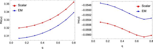
Table 8. Variation of amplitude and damping of QNMs with respect to the charge parameter. |
| a = 0.2, n = 0, ℓ = 2, α = 0.2, η = 0.2 | ||
|---|---|---|
| q | Scalar | EM |
| 0.1 | 0.319889 − 0.0554904i | 0.306802 − 0.0547214i |
| 0.2 | 0.321148 − 0.0555469i | 0.308045 − 0.0547810i |
| 0.3 | 0.323294 − 0.0556375i | 0.310168 − 0.0548770i |
| 0.4 | 0.326408 − 0.0557555i | 0.313252 − 0.0550030i |
| 0.5 | 0.330616 − 0.0558888i | 0.317423 − 0.0551465i |
| 0.6 | 0.336110 − 0.0560148i | 0.322878 − 0.0552860i |
| 0.7 | 0.343183 − 0.0560903i | 0.329915 − 0.0553782i |
| 0.8 | 0.352294 − 0.0560271i | 0.339009 − 0.0553340i |
Figure 15. Variation of amplitude and damping of QNMs with respect to the GM parameter η for scalar and EM perturbations. |
Figure 16. Variation of amplitude and damping of QNMs with respect to the length scale parameter α for scalar and EM perturbations. |
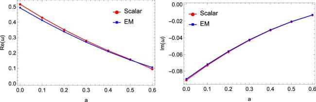
Figure 17. Variation of amplitude and damping of QNMs with respect to the CS parameter a for scalar and EM perturbations. |
Figure 18. Variation of amplitude and damping of QNMs with respect to the charge parameter q for scalar and EM perturbations. |
The QNM frequencies presented in tables 5–8 consist of a real part, representing the oscillation frequency, and an imaginary part, representing the damping rate. The negative imaginary component indicates stability of the perturbations since it ensures that the oscillations decay exponentially with time rather than growing undoubtedly. This confirms the stability of the Frolov BH with GM and CS against scalar and EM perturbations, at least within the parameter ranges considered in this study.
The real part of the QNM frequency, Re(ω), which specifies the oscillation frequency of the perturbations, decreases as the GM parameter η increases. This tendency implies that the oscillation frequency of the perturbations gradually decreases, resulting in a decreased response of the BH spacetime. In contrast, when η increases, the imaginary part Im(ω), which represents the dissipative rate of the oscillations, becomes less negative. This suggests a slower dissipation rate of the disturbances, implying that the oscillations will persist for a longer period of time. A similar pattern is observed for the CS parameter a.
The study also examines the QNM frequencies in relation to the length scale parameter α and charge q. As α increases, Re(ω) rises, indicating more stable oscillations at higher levels. As α increases, Im(ω) decreases, and perturbations dissipate more slowly. The charge q has the opposite effect on QNM frequencies compared to α. As q increases, so does Re(ω), indicating quicker oscillations. As q increases, Im(ω) becomes less negative, indicating slower decay of disturbances. The EM field associated with the charge parameter ‘tightens’ the effective potential around the BH, enhancing the oscillatory response and duration of the oscillations.
The trends observed in the QNM spectra have significant physical implications. The slower damping rates associated with increasing topological defect parameters suggest that BHs with substantial GM and CS components would exhibit longer-lived ringdown signals following perturbation events such as binary mergers. This extended ringdown phase could potentially provide a distinctive observational signature in gravitational wave data, offering a means to identify or constrain the presence of topological defects in astrophysical BHs [80]. Furthermore, the parameter-dependent behavior of the QNM frequencies reveals the intricate interplay between the regular core structure, EM field and topological defects in shaping the spectral characteristics of the BH.
7. Conclusion
In this study, we have presented a comprehensive investigation of the Frolov BH with GM and CS. We explored the combined effects of a non-singular BH core, as introduced by Frolov, and the modifications induced by topological defects. Our study systematically analyzed the geometric, thermodynamic and perturbative properties of the composite spacetime, providing new insights into how the parameters α, q, η and a interact to shape the BH characteristics.
We began by deriving the spacetime metric given by equation (13 ) and the associated metric function ${ \mathcal F }(r)$ in equation (14 ). This formulation encapsulated both the regularizing feature introduced by the Frolov parameter α and the contributions of the GM and CS, represented by the parameters η and a, respectively. Through numerical methods, we demonstrated that the lapse function and the corresponding horizon structure were significantly modified compared to standard BHs. Figures 1, 2 and 3 illustrate how the inner and outer horizons are affected by variations in α, q, a and η, confirming that the presence of topological defects induced notable deviations from the classical RN solution.
In our thermodynamic analysis, we derived the mass function in equation (49 ) by imposing the horizon condition ${ \mathcal F }({r}_{+})=0$, which allowed us to express the BH mass MH as a function of the horizon radius r+ and the model parameters. Figure 7 demonstrated that the mass function reached a minimum at a critical horizon radius before increasing monotonically, a behavior that paralleled the trends observed in both the original Frolov and RN BHs. This result not only validated our approach but also highlighted the intricate balance between the regularization parameter and the effects of the topological defects.
The Hawking temperature, derived in equation (50 ), was shown to depend sensitively on the horizon radius as well as on α, q, a and η. Figure 8 depicts a temperature profile that increased with r+ until reaching a peak, followed by a subsequent decline. This peak shifted with variations in α and q, indicating that the interplay between the EM charge and the regularization parameter plays a crucial role in dictating the BH’s evaporation dynamics. In the appropriate limits, our temperature expression reduced to that of the original Frolov BH or the standard RN solution, thus providing a consistency check for our model.
We computed the entropy via the first law of thermodynamics, leading to the expression in equation (53 ). Unlike the conventional Bekenstein–Hawking area law, the entropy here included logarithmic corrections and additional terms arising from the modified causal structure due to the presence of the GM and CS. This deviation suggests that the information content of the BH is influenced by the topological defects, potentially offering a resolution to aspects of the information paradox [62, 81].
The analysis of the specific heat capacity, given by equation (54 ), revealed further subtleties in the thermodynamic behavior. Figures 9 and 10 clearly show that the specific heat diverged at critical horizon radii, signaling phase transitions between thermodynamically stable and unstable regions. In particular, we observed that the BH exhibited a stable phase within a certain range of r+ (between r1 and r2), beyond which it became unstable. These phase transitions were markedly influenced by the parameters α, a and η, implying that the topological defects not only alter the gravitational field but also have profound implications for the thermal stability and evolution of the BH [63].
Our study also extended to the observational signatures of the BH through the analysis of its shadow. By determining the photon sphere via the condition ${r}_{\mathrm{ph}}{{ \mathcal F }}^{{\prime} }({r}_{\mathrm{ph}})=2{ \mathcal F }({r}_{\mathrm{ph}})$ and computing the shadow radius using equation (60 ), we were able to generate numerical predictions for the apparent size of the BH. Tables 3 and 4 provide detailed numerical values of the photon sphere and shadow radii under different parameter configurations, while figures 11 and 12 offer clear visualizations of how the shadow radius varies with α, q, a and η. Notably, our results demonstrate that while an increase in the Frolov parameters α and q tended to decrease the shadow radius, the incorporation of topological defects (i.e. increasing η and a) led to a significant enlargement of the shadow. This opposing trend could serve as a distinctive observational signature to differentiate between classical and modified BH models.
Finally, we thoroughly explored the dynamics of scalar and EM perturbations around the composite BH spacetime. By solving the massless Klein–Gordon and Maxwell equations, we derived and analyzed the effective potentials for scalar and EM perturbations both analytically and numerically. Our findings indicate that the height and width of the perturbative potentials are significantly sensitive to variations in the GM and CS parameters, whereas the impacts of the Frolov length scale α and electric charge q are comparatively mild, as clearly shown in figures 13 and 14. Utilizing the sixth-order WKB approximation method, we computed the QNMs for both scalar and EM perturbations. Our comprehensive analysis (see tables 5–8 and figures 15–18) reveal that increasing the GM and CS parameters leads to notable decreases in both the oscillation frequencies and the decay rates of the perturbations, reflecting slower damping and prolonged ringdown phases. Importantly, this behavior was consistent across both scalar and EM perturbations, reinforcing the overall stability of the Frolov BH solutions modified by GM and CS. These extended ringdown signatures in gravitational wave observations could serve as distinctive indicators for the presence of topological defects in astrophysical BHs [34].
In summary, our study successfully combines analytical and numerical methods to explore the multifaceted properties of the Frolov BH modified by GM and CS defects. We demonstrate that the inclusion of these topological defects significantly alters the horizon structure, thermodynamic behavior, shadow characteristics and perturbative dynamics of the BH. Our findings not only corroborate known limits, reducing to standard Frolov or RN BHs under appropriate conditions, but also reveal novel features that could be probed in future observational campaigns.
Looking forward, we plan to extend this study in several directions. First, we will consider additional perturbative analyses, such as gravitational perturbations, which are expected to provide further insights into the dynamical stability of these exotic objects. Second, we aim to explore rotating configurations of the Frolov BH with GM and CS since rotation is an essential feature of astrophysical BHs [82]. Finally, we plan to employ advanced numerical techniques and higher-order corrections to refine our QNM calculations and to simulate more realistic scenarios that could be compared with future gravitational wave observations [1].
Appendix. Derivation of the NLED Lagrangian ${{ \mathcal L }}_{{\rm{NLED}}}$ of the Frolov BH
In this appendix, we summarize the derivation of the NLED Lagrangian ${{ \mathcal L }}_{{\rm{NLED}}}$ corresponding to the charged Frolov BH. The goal is to determine the electromagnetic Lagrangian that sources the regular metric function:
$\begin{eqnarray}{ \mathcal F }(r)=1-\frac{(2Mr-{q}^{2}){r}^{2}}{{r}^{4}+(2Mr+{q}^{2}){\alpha }^{2}},\end{eqnarray}$
where M is the mass, q the electric (or magnetic) charge and α is the regularization length scale.A.1. Field equations and ansatz
We consider the action:
$\begin{eqnarray}S=\int {{\rm{d}}}^{4}x\sqrt{-g}\left(\frac{R}{16\pi }+{{ \mathcal L }}_{{\rm{NLED}}}(F)\right),\end{eqnarray}$
with $F=\frac{1}{4}{F}_{\mu \nu }{F}^{\mu \nu }$ being the electromagnetic field invariant.For a purely magnetic field, with magnetic charge q, we use the spherically symmetric field strength:
$\begin{eqnarray}{F}_{\theta \phi }=q\sin \theta ,\quad \Rightarrow \quad F=\frac{{q}^{2}}{{r}^{4}}.\end{eqnarray}$
The Einstein equations yield the relation:
$\begin{eqnarray}{G}_{0}^{0}={G}_{1}^{1}=\frac{r{f}^{{\prime} }(r)-1+f(r)}{{r}^{2}}=8\pi {T}_{0}^{0}=2{ \mathcal L },\end{eqnarray}$
from which the Lagrangian can be written as, $\begin{eqnarray}{ \mathcal L }(r)=\frac{r{f}^{{\prime} }(r)-1+f(r)}{2{r}^{2}}.\end{eqnarray}$
A.2. Substituting the metric function
Given the lapse function:
$\begin{eqnarray}f(r)=1-\frac{{r}^{2}(2Mr-{q}^{2})}{{r}^{4}+(2Mr+{q}^{2}){\alpha }^{2}},\end{eqnarray}$
where its derivative with respect to r yields a rational expression. Substituting into the expression for ${ \mathcal L }(r)$ gives: $\begin{eqnarray}{ \mathcal L }(r)=-\frac{12{M}^{2}{\alpha }^{2}{r}^{2}+4M{q}^{2}{\alpha }^{2}r-3{q}^{4}{\alpha }^{2}+{q}^{2}{r}^{4}}{2{\left(2M{\alpha }^{2}r+{q}^{2}{\alpha }^{2}+{r}^{4}\right)}^{2}}.\end{eqnarray}$
A.3. Final expression for ${{ \mathcal L }}_{{\rm{NLED}}}(F)$
Since $F=\frac{{q}^{2}}{{r}^{4}}$, we solve for r in terms of F:
$\begin{eqnarray}r={\left(\frac{{q}^{2}}{F}\right)}^{1/4}.\end{eqnarray}$
The corresponding NLED Lagrangian in terms of F becomes: $\begin{eqnarray}\begin{array}{l}{ \mathcal L }(r)\to {{ \mathcal L }}_{{\rm{NLED}}}(F)\\ \quad =-\frac{1}{2}\frac{12{M}^{2}{\alpha }^{2}\sqrt{\frac{{q}^{2}}{F}}+4M{q}^{2}{\alpha }^{2}{\left(\frac{{q}^{2}}{F}\right)}^{1/4}-3{q}^{4}{\alpha }^{2}+\frac{{q}^{4}}{F}}{{\left(2M{\alpha }^{2}{\left(\frac{{q}^{2}}{F}\right)}^{1/4}+{q}^{2}{\alpha }^{2}+\frac{{q}^{2}}{F}\right)}^{2}}.\end{array}\end{eqnarray}$
This expression ensures that the Einstein equations are satisfied by the metric function ${ \mathcal F }(r)$. Moreover, ${{ \mathcal L }}_{{\rm{NLED}}}$ is finite at r = 0 and asymptotically approaches the standard Maxwell form ∼F as r → ∞, confirming its consistency as a NLED source for regular BH spacetimes.