This study examines the effect of charge on physical features of a gravastar model in the framework of Rastall gravity. A gravastar is an alternative model to a black hole consisting of three separate regions: the inner sector, the intermediate shell and the outer sector. Different values of the barotropic equation of state (EoS) parameter provide the mathematical basis for these regions. Field equations (FEs) are initially developed for a spherically symmetric spacetime coupled with charged matter distribution. We then use the temporal component of Tolman IV spacetime to formulate the radial metric potential for both the inner region and intermediate shell. We also apply the matching criteria to ensure smooth matching of exterior and interior spacetimes so that the constants resulting from integrations can be determined. Afterwards, we explore various physical properties of the developed gravastar model such as the proper length, entropy, energy, and others to analyze how shell thickness and charge affect them. It is concluded that, in the background of Rastall theory, a gravastar model exists and serves as a viable alternative to the black hole.
M. Sharif, Tayyab Naseer, Areej Tabassum. Exploring structure and stability of charged gravastar in non-conservative theory of gravity[J]. Communications in Theoretical Physics, 2026, 78(2): 025406. DOI: 10.1088/1572-9494/ae0158
1. Introduction
Compact cosmic remnants represent the ultimate outcome of stellar formation. When a star’s thermal pressure no longer counterbalances the force of gravity, it forms a compact object. Due to the extreme pressure and density conditions created by this ultimate collapse, astrophysicists have shown great interest in studying these objects and their evolution. This provides a valuable opportunity to test various theories within the realm of general relativity (GR). It is hypothesized that when a massive star undergoes a supernova explosion, the remnant’s mass determines whether it becomes a neutron star or a black hole [1]. Karl Schwarzschild presented the first solution for black holes derived from Einstein’s field equations (FEs) within a vacuum scenario in 1916 [2]. This solution is pivotal for both charged and uncharged classical black holes. However, the Schwarzschild solution has two significant issues: (i) a central singularity, and (ii) an event horizon. The central singularity, which occurs as r approaches zero, is an irreducible feature that cannot be removed, even through coordinate transformations; it is termed a dynamical singularity [3]. In contrast, the other singularity, $r={r}_{{\rm{s}}}=\frac{2GM}{{c}^{2}}$, corresponding to the event horizon located at r = 2M (with G = 1 = c) is a coordinate singularity and introduces notable complexities [3]. In quantum mechanics, this event horizon suggests that a photon’s energy becomes infinite near this point, with no predefined parameters available to control this divergence.
Although GR provides a framework for understanding cosmic phenomena, it falls short in explaining the Universe’s accelerated expansion. This shortfall arises from well-known problems like fine-tuning and the cosmic coincidence issue. To tackle these problems along with the singularity issue, several modifications to GR have been proposed. In connection with this, Rastall [4, 5] put forward an intriguing modification to GR in 1972, gaining attention from numerous researchers. His approach challenges the traditional conservation law of the energy-momentum tensor (EMT), i.e. ∇νTμν = 0 in curved spacetime, suggesting that this law may not always hold. Instead, Rastall’s theory posits that the covariant divergence of the EMT is proportional to the derivative of the scalar curvature expressed by ∇νTμν ∝ R,μ. He introduced a coupling parameter, where a zero value returns the theory to standard GR. Additionally, Rastall’s FEs are simpler than those in other modified theories, making them easier to solve and analyze.
Rastall gravity (RG) offers a simple version of Einstein's FEs that reveal intriguing characteristics from both astrophysical and cosmological viewpoints. Recently, this theory has proven effective in formulating the geometry of different black hole solutions, including charged, uncharged and rotating black holes [6–10]. This theory has also played a significant role in generating the compact stars model. Mota et al [11] explored the physical existence and properties of neutron stars to examine how they behave in the context of Rastall theory. Abbas and Shahzad [12] investigated a novel solution for an anisotropic compact star under this non-conserved theory with a varying cosmological constant, as well as Krori–Barua metric components [13]. Oliveira et al [14] have also determined spherically symmetric solutions representing the interior of a neutron star in this theory and found consistent outcomes. The particular choices of the Rastall parameter have been taken into account to determine the physical traits of a compact star PSR J0740+6620 and concluded that this star maintains its stability under sound speed constraints [15]. Hansraj et al [16] examined the effects of the Rastall parameter to explore its implications for modeling neutron stars and cold fluid structures. Additionally, the role of the non-conservation phenomenon has been extensively examined in various stellar models in the literature [17–23].
A hypothetical, highly compact object devoid of singularity, known as a gravastar, has been proposed as a potential alternative to black holes. This concept could be developed by exploring the fundamental principles of Bose–Einstein condensation. Mazur and Mottola [24] introduced a distinctive model, which offers a solution to Einstein‘s FEs. They named this entity a gravitationally condensate star, or gravastar. Several scholars have shown interest in investigating the structure of a gravastar because this model is anticipated to address two critical problems related to black hole structure—the information paradox and the formation of singularity. The gravastar structure is divided into three domains: internal, thin-shell, and external. In the inner domain, the state variables have a relation ϱ = − p, where ϱ and p stand for pressure and energy density, respectively. The non-attractive force produced by this matter composition generates sufficient pressure to prevent collapse. The internal area is protected by a central region that contains stiff matter and follows the relation ϱ = p. This shell applies an inward force on the inner area, maintaining hydrostatic balance and creating a compact structure without possessing singularity. The outer region is completely void, adhering to the equation of state (EoS) where both the pressure and density are zero, expressed as ϱ = p = 0.
Although there is no direct experimental confirmation of gravastars, indirect evidence hints at their potential existence. Sakai et al [25] established criteria for detecting gravastars through the analysis of their shadows. Kubo and Sakai [26] attempted to identify gravastars through gravitational lensing by detecting peak luminosity effects, which are absent in black holes of the same mass. Additionally, the cosmic event GW150914, observed by LIGO interferometers, detected a ringdown signal [27, 28]. The objects emitting these signals do not possess an event horizon, suggesting the presence of gravastars. A recent image from the Event Horizon Telescope (EHT) has been examined that pointed to the existence of such objects [29]. Visser and Wiltshire [30] developed a simplified model of the gravastar, analyzed its dynamic stability and found that certain EoSs for the transition layer result in a stable configuration. Carter [31] derived new spherically symmetric gravastar solutions which are stable under radial perturbations. Horvat and Ilijic [32] proposed such a model and analyzed configurations with stiff, dust, and tension shells. They also examined the stability of their resulting models by taking into account two different (such as Schwarzschild and Schwarzschild-de Sitter) exteriors. There is a wide range of studies on gravastar solutions, investigating various matter contents [33–38]. Some fascinating explorations across diverse fields can be found in the literature [39–42].
Ghosh et al [43] examined a new gravastar model in higher-dimensional spacetime and suggested that such models may not be physically applicable. Abbas and Majeed [44] developed a new gravastar model using the Mazur–Mottola mechanism, featuring a stable, three-layers structure with singularity-free interior. Debnath [45] further explored charged gravastars in the Rastall–Rainbow gravity framework, examining stability and key physical properties. Majeed and Abbas [46] extended this work and found exact, stable and non-singular gravastar solutions in non-conservative RG using the Kuchowicz metric potentials. Bhattacharjee and Chattopadhyay [47] investigated the impact of charge on isotropic spherically symmetric gravastars and explored their structural characteristics. The remarkable discoveries of gravastars have prompted experts to investigate their structural properties within modified theories [48–52].
Electromagnetism is essential for understanding the structural development and stability of collapsing cosmic entities. To maintain the balance of a stellar body, a considerable quantity of charge is necessary to counteract gravitational forces. Lobo and Arellano [53] explored various gravastar models within nonlinear electrodynamics, constructing electrically and magnetically charged gravastars, and examined their physical properties. Horvat et al [54] extended this model by introducing an electrically charged component and analyzed the impact of the electromagnetic field on the sound speed and surface redshift. Turimov et al [55] analyzed dipolar magnetic fields and Maxwell equations in the interior of a slowly rotating gravastar. Usmani et al [56] introduced a model possessing conformal motion and internal charge by taking into account the Reissner–Nordström exterior metric. Some other works in the presence of charge are [57–68]. One can think that the charged core acts as an electromagnetic mass model which is crucial for the gravastar’s stability. Sharif and Javed [69] examined the stability of the gravastar within the context of quintessence and conventional black hole geometries, revealing a continuously increasing trend in physical characteristics against the shell’s thickness. Various metric ansatz have been suggested in the literature and used by astrophysicists to develop physically viable structures. In this regard, Tolman IV spacetime gained much significance in the literature [70]. Recent studies related to this metric have been examined in [71–74].
This study investigates the effect of charge on the gravastar model in the context of RG. We explore the structure of this object containing three different domains within the framework of Tolman IV spacetime and graphically represent its physical characteristics. The paper is structured as follows. Section 2 outlines the core concepts and definitions of the considered non-conserved theory, taking into account the impact of an electric charge on the geometry of spherical spacetime. Section 3 explores the structure of a charged gravastar by analyzing the relevant EoSs for each region. Sections 4 and 5 delve into the physical traits of the developed gravastar model, covering aspects such as the proper length, energy, EoS parameter, entropy, and structural stability. The final section provides a summary of our main findings.
2. Non-conserved Rastall FEs
In Einstein’s GR, the conservation law for the EMT is expressed as ${T}_{\mu ;\nu }^{\nu }=0$. Peter Rastall extended this theory by modifying this conservation law in curved spacetime [4]; it is formulated as follows
where λ is a constant and R = gμνRμν represents the Ricci scalar. Within the framework of RG, the constant λ can be seen as quantifying the tendency to which the geometry interacts with the matter fields. This interaction results in a revised form of FEs, expressed as
with κ being the gravitational coupling parameter. For the current case, we eliminate $\kappa \lambda =\frac{1}{4}$ because it results in T = 0 and R = 0, which effectively reduces to Einstein’s theory where Rμν = 0. The dimensionless Rastall parameter, denoted by χ, is defined as the product of the Rastall and gravitational coupling parameters, i.e. χ = κλ. Hence, in a relativistic unit system, where G and c are set to unity, the simplified form of κ and λ are given by
Equation (5) shows that when χ = 0, κ satisfies Einstein’s gravitational constant. This also shows that for $\chi =\frac{1}{6}$, κ diverges, and therefore we restrict $\chi =\frac{1}{4}$ for RG specifications. Finally, by using equations (2)–(5), Rastall's FEs are formulated as follows
To study the charged gravastar in relativistic astrophysics, we consider a spherically symmetric and static spacetime. In Schwarzschild coordinates, the general form of the line element can be expressed as
where the two functions ξ = ξ(r) and γ = γ(r) denote the gravitational potentials. Assuming the fluid source is comprised of normal matter and is surrounded by the electromagnetic field, the EMT can be represented as
In the equation given above, uμ represents the fluid’s four-velocity, which satisfies the condition uμuμ = − 1. Moreover, the symbols ϱ and p denote the energy density and pressure of the fluid, respectively.
The EMT for the electromagnetic field is represented as
where Jμ is the current density, satisfying Jμ = σuμ with σ being the charged density. The only non-zero component of Fμν in the current scenario is F01 = −F10, which is a function of the radial coordinate alone. Thus, from equation (12) (left), we can derive the following expression for the interior charge q(r) as
It is worth mentioning here that when the Rastall parameter χ → 0, this theory and the corresponding results reduce to GR.
3. Gravastar geometry
In this section, we examine the geometry of the charged gravastar model by analyzing three distinct regions: the interior domain, the thin shell, and the exterior domain, each of them governed by specific EoSs. The thin shell, having an insignificant thickness, surrounds the inner layer of the gravastar. This shell extends from R1 = R < r to R2 = R + ε with the small thickness represented by ε = R2 − R1. Note that the radii of the interior and exterior layers of the charged gravastar are denoted by R1 and R2, respectively.
3.1. Inner domain
The core of a charged gravastar is believed to be a de Sitter vacuum characterized by the EoS p = −ϱ. The repulsive force arising from the negative pressure in this region counteracts the inward gravitational pull on the shell. However, this region’s negative energy density is analogous to a positive cosmological constant. The ‘degenerate vacuum’ is a specific type of EoS that is commonly used to describe dark energy systems. Substituting the EoS for the interior region in the non-conservation equation (17) results in
Here, ${k}_{1}=\kappa {\varrho }_{{\rm{c}}}\left(1+\frac{4\chi -1}{4\chi }\right)$ and k2 is an integration constant. If we set k2 to be zero, the solution will be regular at r = 0, resulting in the simplified form given by
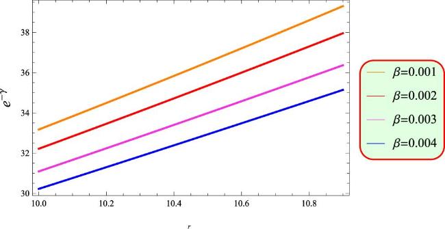
The previous analysis indicates that the interior region’s solution is devoid of singularities, effectively overcoming the singularity problem commonly found in conventional black hole models. To graphically plot the factor (20), we need to make the interior charge a known quantity. It has initially been taken as $q(r)={q}_{0}{\left(\frac{r}{R}\right)}^{n}$ with n and q0 being constants, and R denoting the object’s boundary [75]. Later, a new form of this quantity has been suggested in which n was fixed to be 3 and $\beta =\frac{{q}_{0}}{R}$; it therefore takes the form q = βr3. This choice has widely been used in the literature to simplify the governing equations characterizing charged fluid distributions [76–78]. Figure 1 shows the singularity-free increasing behavior of the component (20) for distinct values of β. To examine the active gravitational mass of the inner sector, we employ the following equation
Figure 1. Metric component (20) versus r for different values of β.
3.2. Intermediate region
A charged gravastar’s non-vacuum shell is filled with a highly relativistic fluid that exhibits an EoS defined by p = ϱ. This form of matter, referred to as stiff matter, was initially introduced by Zel’dovich in connection with a cold baryonic universe [79]. Several researchers have utilized this form of matter distribution and achieved notable findings [80–84]. Some ground-breaking work in various other disciplines can be found in [85–88]. However, within the specified limit for this zone, i.e. 0 < e−γ(r) ≪ 1, such possibilities can be derived by taking into account the EoS for the thin layer. The smooth transition between the inner and outer parts of a charged gravastar leads to a thin shell structure representing the intermediate region. Incorporating this constraint, the system (14)–(16) becomes
GR has greatly enhanced our understanding of the cosmos by revealing numerous astrophysical phenomena. One notable model, the gravastar structure, requires explicit solutions to explore its gravitational characteristics. Scholars have employed several methods to address the FEs, including the Finch–Skea condition, the Tolman–Kuchowicz metric ansatz, and conformal motion, etc. In this study, we utilize the Tolman IV metric potential, focusing particularly on its temporal component, which consists of a set of constants. This allows us to create a model analogous to the gravastar structure. Richard C. Tolman [70] developed this ansatz, a mathematical framework that effectively characterizes the gravitational field resulting from a specific distribution of matter. The expression for the gtt potential in connection with the Tolman IV metric is given as follows
It must be highlighted that there are two approaches to solve the Rastall FEs. Since there are three governing equations (23)–(25) along with the EoS for the thin shell, i.e. p = ϱ, we can solve them to find a unique solution as the number of unknowns are also four. However, this has already been done in the literature. We, therefore, apply another approach by taking into account the fact that the isotropic fluid composition can be completely expressed with the help of equations (23) and (24). These two equations along with p = ϱ contain four unknowns (two metric potentials, isotropic pressure and energy density). To solve this system uniquely, we consider the time component of Tolman IV spacetime (26) as the fourth equation. This choice simplifies the mathematical treatment and fits well with the unique characteristics of the thin shell region in the gravastar model. Utilizing equations (23), (24) and (26) together with the EoS p = ϱ, we calculate the inverse radial metric potential for the thin shell as
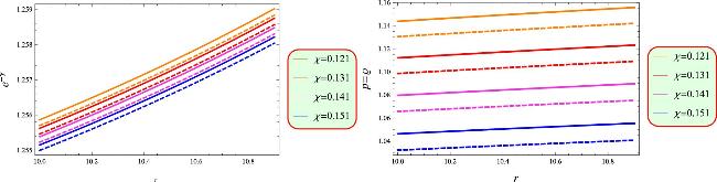
where $\varpi =A\left(48{\chi }^{3}+28{\chi }^{2}-1\right)$. Here, the integration constant is denoted by C, and the radius r lies within the interval R1 = R < r and R2 = R + ε > r along with the considerations ε ≪ 1 and e−γ ≪ 1. Figure 2 shows how the metric potential eγ behaves consistently over the intermediate shell r. By substituting the EoS p = ϱ and (26) into (17), we derive the expression for density (such that density = pressure) as follows
It can be observed that the density is directly related to the radius. This indicates that the high-relativistic fluid in the shell of the gravastar is denser in the outer regions as compared to the inner ones. Figure 2 depicts the evolution of energy density, showing that as we move away from the center, the fluid becomes even denser. In contrast, when we increase the value of charge, the fluid gets less dense as compared to the lower charge, indicating that the higher electric charge enhances the shell’s density and possibly its stability.
Figure 2. Metric component (27) and pressure (28) versus r for Q = 1.23 (solid) and 1.25 (dashed).
3.3. Outer layer
This sector is characterized by the EoS ϱ = 0 = p, implying that pressure and density are both zero. Hence, the outer sector indicates a vacuum. Since the interior spherical geometry is charged, the most suitable line element indicating the exterior region is the Reissner–Nordström metric. This is described as follows
where M and Q refer to the total exterior mass and charge, respectively.
3.4. Boundary conditions
A gravastar structure is characterized by two primary boundaries: one boundary is located at r = R1, defining the interface between the inner and intermediate regions, while the other boundary is at r = R2, differentiating the outer layer from the gravastar’s shell. By equating the metric functions at these boundaries, we can derive the values of arbitrary constants A, B and C involved in the assumptions made previously. Both the metric potentials and the radial derivative of the gtt component are matched at R = R2 to ensure continuity. This results in three distinct equations, which are given as follows
In this study, we analyze a charged gravastar model by selecting specific Rastall parametric values. We use a mass of M = 3M⊙ and an outer boundary radius of R2 = 10.9 km, with different values of χ as 0.121, 0.131, 0.141, and 0.151. It must be mentioned here that some thermodynamical studies in Rastall theory suggest that the parameter χ must be less than 0.16 or greater than 0.25 [89]. We thus chose the above four values to ensure our study was consistent with the previous findings. By utilizing these parameters, we compute the constant triplet A, B, C for two distinct charge values, as presented in tables 1 and 2. Our findings indicate that the constant C varies with the electric charge and Rastall parameter, while A and B change only with respect to the charge. We ensure that the condition $\frac{2M}{{R}_{2}}\lt \frac{8}{9}$ is satisfied. This constraint allows for the selection of different combinations for M and R2 that yield acceptable results. Consequently, this particular relationship between the radius and mass leads to a distinct outcome when the charge varies.
Table 1. Numerical values of constant triplet for Q = 1.23 with M = 3M⊙ and R2 = 10.9.
χ
A
B
C
0.1201
90.4236
0.199779
0.410164
0.1202
90.4236
0.199779
0.409312
0.1203
90.4236
0.199779
0.408394
0.1204
90.4236
0.199779
0.407442
Table 2. Numerical values of constant triplet for Q = 1.25 with M = 3M⊙ and R2 = 10.9.
χ
A
B
C
0.1201
91.0784
0.200825
0.411031
0.1202
91.0784
0.200825
0.410168
0.1203
91.0784
0.200825
0.409263
0.1204
91.0784
0.200825
0.408313
4. Core features of the gravastar model
The gravastar model offers insights into the nature of compact objects and challenges conventional understandings of gravitational phenomena. This section examines the properties of a charged gravastar, specifically its proper length, shell energy, entropy and EoS parameter through graphical analysis. We shall explore how different positive values of the Rastall parameter and charge affect these characteristics.
4.1. Proper length
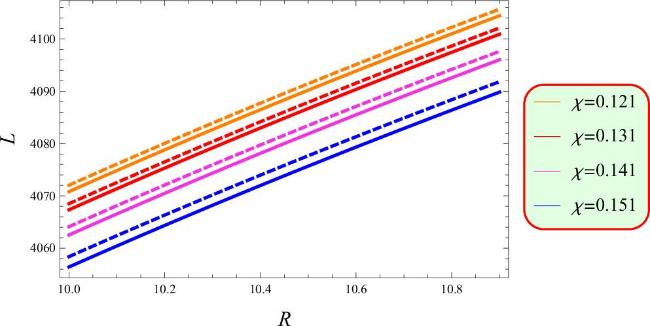
The proper length of the central region is given by R2 − R1 = ε, where ε is a small quantity indicating an insignificant change. The formula for the length of the thin shell is given by
We use Taylor series approximation (up to the second order of the thickness parameter, i.e. ε2) to estimate the length of the thin shell. After performing some mathematical steps and manipulating them (for details, see [90]), we ultimately determine the shell’s length as follows
The graphical description of the shell’s length is displayed in figure 3. This illustrates an increment in the thin shell length as the radius value rises. Figure 3 also reveals that increasing the charge within the fluid increases the shell length, suggesting that the electromagnetic field expands the gravastar’s shell. Consequently, uncharged gravastars exhibit a relatively shorter shell length.
Figure 3. Proper length versus R for Q = 1.23 (solid) and 1.25 (dashed).
4.2. Energy of charged shell
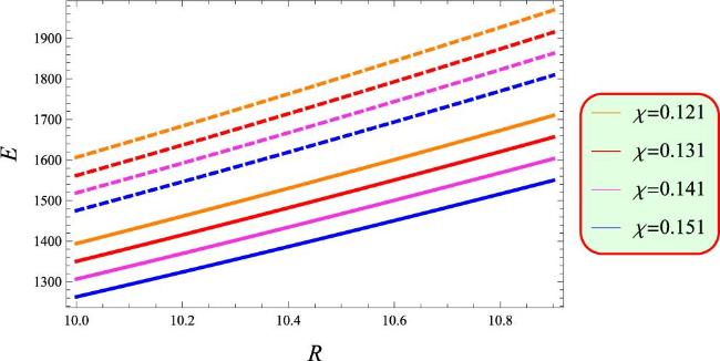
The core of a charged gravastar exhibits repulsive behavior, characterized by the EoS ϱ = −p. The observed negative pressure, indicative of dark energy, generates the repulsive force. The energy associated with this behavior is mathematically represented as follows
Since the above integration is not easy to solve analytically, we use numerical methods to examine the impact of the electromagnetic field on the energy within the shell. Figure 4 illustrates that the energy increases by increasing the shell’s radius. It is also found that the energy is directly proportional to both Rastall parameter and charge as their increasing values result in the gravastar model possessing higher energy. This boost in energy enhances the shell’s repulsive forces, improving stability against gravitational collapse.
Figure 4. Energy versus R for Q = 1.23 (solid) and 1.25 (dashed).
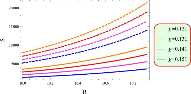
4.3. Entropy
The entropy of a gravastar is an intriguing aspect that reflects its unique structure and physical properties. In the interior region of a gravastar, the entropy density is found to be zero, indicating a state of minimal disorder within this domain. However, within the thin shell that encases this interior, the entropy can be expressed through specific mathematical formulations, revealing that it is influenced by local temperature variations. This thin shell, composed of ultra-relativistic matter, plays a crucial role in maintaining stability and contributes to the overall entropy of the gravastar. The formula to calculate the entropy is given by
$\begin{eqnarray}S={\int }_{R}^{R+\epsilon }4\pi {r}^{2}{ \mathcal X }(r)\sqrt{{{\rm{e}}}^{\gamma (r)}}{\rm{d}}r,\end{eqnarray}$
where ${ \mathcal X }(r)$ is the entropy density which is defined in terms of the local temperature t(r) as
$\begin{eqnarray}{ \mathcal X }(r)=\frac{{\vartheta }^{2}{{K}_{{\rm{B}}}}^{2}t(r)}{4\pi {\hslash }^{2}}=\vartheta \left(\frac{{K}_{{\rm{B}}}}{\hslash }\right)\sqrt{\frac{p}{2\pi }},\end{eqnarray}$
with KB and ℏ being constants. Using equations (28), (46) and (48) together results in
Analytically solving the above equation is difficult, so we turn to a numerical approach. Figure 5 illustrates that the entropy of the gravastar shell rises with increasing shell’s radius, reaching its maximum value at the outer surface. The entropy is influenced by higher charge density and local temperature variations, potentially enhancing the gravastar’s stability. Moreover, the higher values of χ and the charge also lead to the greater entropy in the context of Rastall theory.
Figure 5. Entropy versus R for Q = 1.23 (solid) and 1.25 (dashed).
4.4. Junction conditions
To study celestial bodies, it is essential to smoothly match the interior and exterior spacetimes. The charged gravastar structure consists of three main regions, denoted as R1, R, and R2, with R serving as the interface between R1 and R2. The Israel matching criterion [91] ensures the smooth alignment of the inner and outer geometries. While the metric coefficients remain continuous, their derivatives may exhibit discontinuities at the hypersurface. Based on Lanczos equations [92], the stress-energy tensor for the matter surface is determined as
$\begin{eqnarray}{S}_{\alpha }^{\lambda }=-\frac{1}{8\pi }[{{ \mathcal K }}_{\alpha }^{\lambda }-{\partial }_{\alpha }^{\lambda }{{ \mathcal K }}_{n}^{n}].\end{eqnarray}$
The extrinsic curvature admits a discontinuity given by
$\begin{eqnarray}{{ \mathcal K }}_{\lambda \alpha }={{ \mathcal K }}_{\lambda \alpha }^{+}-{{ \mathcal K }}_{\lambda \alpha }^{-},\quad \lambda ,\alpha =0,2,3,\end{eqnarray}$
where λ and α represent the coordinates on the hypersurface. The extrinsic curvature associated with R1 and R2 is given as
The condition ηkηk = 1 holds, where ζα denotes the inherent coordinates on the shell. The parametric equation of the shell is described by f(Xα(χi)) = 0. The symbols − and + refer to the spherical interior metric and the Reissner–Nordström spacetime, respectively.
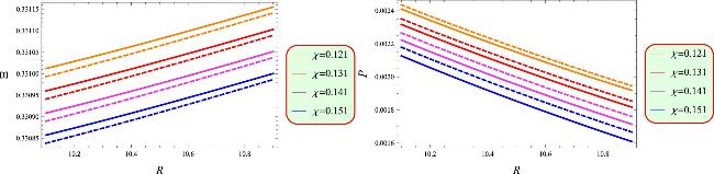
According to the Lanczos equation, the tensor Sλα is represented as Sλα = diag( −Ξ, P, P, P), where Ξ corresponds to the surface energy density, and P signifies the surface pressure. The equations below define Ξ and P as follows
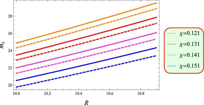
Figure 6 represents the graphs of both these physical quantities as functions of the radius R. The plots reveal that the energy density and pressure are directly and inversely proportional to the radius, respectively. Moreover, as both the Rastall parameter and the charge increase, the energy density decreases, while the surface pressure increases. These observations support the validity of the model which allow us to proceed further to calculate the thin shell’s surface mass. Its formula is described by
Figure 7 displays the rising profile of the thin shell’s mass against R, emphasizing a physically viable feature of compact stellar objects. The total mass M of the gravastar, in relation to the thin shell’s mass ms, is expressed as follows
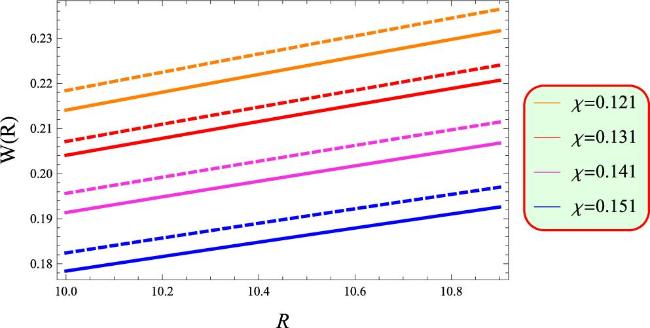
To keep W(R) real, we need to satisfy constraints such as, $\frac{2M}{R}+\frac{{Q}^{2}}{{R}^{2}}\lt 1$ and $\frac{\kappa {\varrho }_{{\rm{c}}}}{3}\left(1+\frac{4\chi }{4\chi -1}\right){R}^{2}-\frac{\kappa {Q}^{2}}{{R}^{2}}\lt 1$. The constraints relating M, Q and R are given by $Q\gt \sqrt{2MR-{R}^{2}}$ and R > 2M. Taking positive values for both surface density and pressure leads to a positive value of W. For large R, we find that W(R) ≈ 1. The structure of the gravastar becomes comparable to compact objects when R is sufficiently large. Additionally, substituting specific values of R into equation (58) can result in W = 0, representing a dust shell. Figure 8 illustrates the plot of the EoS parameter, showing that it remains acceptable under the influence of charge.
Figure 8. EoS parameter versus R for Q = 1.23 (solid) and 1.25 (dashed).
5. Stability
The two main methods used in this section to analyze the stability of our hypothetical charged model representing the gravastar are surface redshift and entropy maximization. These strategies are explained in the following subsections.
5.1. Surface redshift
Examining the surface redshift of a gravastar is essential for evaluating its stability. To calculate the gravastar’s gravitational surface redshift, we use the formula ${Z}_{{\rm{s}}}=\frac{{\rm{\Delta }}\lambda }{{\lambda }_{{\rm{e}}}}=\frac{{\lambda }_{0}-{\lambda }_{{\rm{e}}}}{{\lambda }_{{\rm{e}}}}$, where λ0 is the wavelength emitted by the source and λe is that detected by the observer. According to Buchdahl’s proposal [93], an isotropic, stable, ideal fluid distribution should have a surface redshift of not more than 2. However, Ivanov [94] stated that it might become up to 3.84 for the anisotropic fluid setup. Moreover, Barraco and Hamity [95] demonstrated that for an isotropic fluid distribution without the cosmological constant, the condition Zs ≤ 2 is satisfied. In our case, we define the surface redshift given by
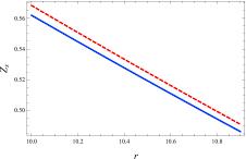
Figure 9 illustrates the variation in the surface redshift within the gravastar model, showing that this factor increases as we increase the value of charge. This indicates that higher charges reduce the gravitational redshifting of light escaping from the gravastar. This effect is likely due to stronger electromagnetic influences counteracting the gravitational pull. Additionally, it is worth noting that the Rastall parameter does not influence the surface redshift.
Figure 9. Surface redshift versus r for Q = 1.23 (solid) and 1.25 (dashed).
5.2. Entropy maximization
This approach maximizes the entropy in relation to the mass function. At the gravastar’s shell boundaries, specifically at r = R1 and r = R2, stability is attained when the entropy functional’s initial variation equals zero which is mathematically denoted by δS = 0. The entropy functional is given as
This paper investigates the construction of a charged gravastar within the context of RG. The gravastar model presents a compelling alternative to traditional black hole theories, characterized by three distinct regions: the interior, the thin shell, and the exterior. The interior region is defined by a negative energy density, leading to a repulsive pressure that counteracts gravitational collapse, i.e. characterized by p = −ϱ. Surrounding this core is the thin shell (represented by ϱ = p), composed of ultra-relativistic matter, which maintains stability by balancing the outward pressure from the interior. Finally, the exterior region is typically represented by a vacuum solution, such as the Reissner–Nordström metric in the case of charged geometrical structure, indicating a non-singular spacetime structure expressed by the EoS ϱ = p = 0.
To discuss this model, we have assumed the spherical spacetime and electromagnetic EMT to induce the effects of charge in the geometry of the gravastar. We have also considered the temporal component of the Tolman IV ansatz to make our complex expressions easy to solve. Using this potential, we have calculated the radial components for both the shell and interior regions. The boundary conditions have afterwards been used to make the constants (having appeared from the Tolman IV ansatz and performing integrations) known. Furthermore, different physical attributes of the gravastar model have been explored to observe how they become influenced by the presence of charge. The key findings of our study are summarized as follows.
The growing density suggests that the outer boundary of the shell is denser as compared to the inner boundary (figure 2).
The proper length of the charged intermediate region increases as the shell’s radius expands (figure 3). The gravastar length continues to grow with increasing charge values.
The energy associated with the inner region is lower compared to that of the outer region. The graph shows that the radius of the shell increases linearly with the energy of the shell (figure 4).
The entropy of a charged thin shell is directly related to its radius; as the shell expands, its entropy increases (figure 5). Additionally, an increase in the electric charge contributes to a rise in the entropy.
A rising trend in surface energy density and declining trend in surface pressure against R are found (figure 6). It is also noted that increasing the electric charge decreases the former and increases the later's surface quantity. Additionally, the continuous increase in the shell’s mass is noted as the radius grows (figure 7).
The EoS parameter shows an acceptable profile under certain conditions, such as $\frac{\kappa {\varrho }_{{\rm{c}}}}{3}\left(1+\frac{4\chi }{4\chi -1}\right){R}^{2}-\frac{\kappa {Q}^{2}}{{R}^{2}}\lt 1$, which helps to maintain the real value of W(R) (figure 8).
The surface redshift confirms the stability of our hypothetical model (figure 9).
Several astrophysical tests could detect the existence of gravastar models. We discuss these tests and how they are affected under the considered non-conserved theory in the following.
Gravastar shadows are similar to black hole shadows, appearing as dark regions against brighter emissions but without an event horizon due to the gravastar’s compact nature. Under RG, these shadows could exhibit variations in size and shape. Such differences are essential for distinguishing gravastars from black holes and for evaluating the accuracy of RG’s predictions.
Microlensing involves a massive object, such as a gravastar, amplifying light from a distant source as it passes between the source and an observer, revealing the presence of compact masses indirectly. Under RG, changes in gravitational interactions could alter the intensity and pattern of microlensing light curves. These deviations from expected patterns could provide unique signatures that distinguish gravastars from black holes.
The EHT is a network of global radio telescopes that takes high-resolution images of the regions around supermassive black hole candidates, capturing the shadow and light rings formed by intense gravitational bending. If gravastars are real and are influenced by RG, the EHT might detect unusual ring-like structures around these objects, differing from typical black hole observations.
LIGO detectors detect spacetime ripples from massive astrophysical events, such as mergers or collapses. If gravastars merge, they too could produce detectable gravitational waves. These waves might display unique characteristics, like altered waveforms or energy distributions, under RG, potentially distinguishing them from black hole signals.
Our findings indicate that charge plays a significant role in shaping the formation and properties of gravastars, suggesting that charged gravastar models are feasible within the framework of RG. The application of this non-conserved theory alters the fundamental characteristics of charged gravastars compared to those predicted by Einstein gravity. It is important to highlight that the shell’s approximation has been taken up to the second order to achieve more accurate outcomes [96]. Moreover, the results of this study are consistent with those of the uncharged version [90]. We conclude that this modified theory effectively describes the behavior of charged gravastar models. Furthermore, setting the Rastall parameter to zero, i.e. χ = 0 reduces these results to GR.
NaseerT, SharifM2024 Role of decoupling and Rastall parameters on Krori–Barua and Tolman IV models generated by isotropization and complexity factor Class. Quantum Grav.41 245006
NaseerT2024 Complexity and isotropization based extended models in the context of electromagnetic field: an implication of minimal gravitational decoupling Eur. Phys. J. C84 1256
NaseerT2025 Isotropization and complexity based extended Krori–Barua and Tolman IV Rastall models under the effect of electromagnetic field Astropart. Phys.166 103073
FengG, YuS, WangT, ZhangZ2025 Discussion on the weak equivalence principle for a Schwarzschild gravitational field based on the light-clock model Ann. Phys.473 169903
NaseerT, SaidJ L2024 Existence of non-singular stellar solutions within the context of electromagnetic field: a comparison between minimal and non-minimal gravity models Eur. Phys. J. C84 808
Zel'dovichY B, SmorodinskyY A1962 On the upper limit on the density of neutrinos, gravitons, and baryons in the universe Sov. Phys. J. Exp. Theor. Phys.14 647
80
CarrB J1975 The primordial black hole mass spectrum Astrophys. J.201 1-9
DingS, LiuC, FanZ, HangJ2025 Lumped parameter adaptation-based automatic MTPA control for IPMSM drives by using stator current impulse response IEEE Trans. Energy Convers. 1-11
ZengZ, GoetzS M2025 A zero common mode voltage PWM scheme with minimum zero-sequence circulating current for two-parallel three-phase two-level converters IEEE J. Emerg. Sel. Top. Power Electron.13 1503-1513
MoradpourH, SalakoI G2016 Thermodynamic analysis of the static spherically symmetric field equations in Rastall theory Adv. High Energy Phys.2016 3492796


