


1. Introduction
General relativity (GR), which presents a structural configuration to comprehend space and time, substitutes the classical Newtonian approach of defining gravity. It is essential in evaluating several events happening in the Universe, incorporating cosmic inflation, cosmic development, and how gravity affects dynamic compact systems. The most persuasive argument for the rapid growth of the entire cosmos is found in the observations of Type Ia supernovae, the cosmic microwave background (CMB), and large-scale structure searches, as demonstrated by the most recent studies [1–4]. This discovery has profound consequences for our comprehension of the Universe’s evolution and the nature of the enigmatic dark energy that seems to be controlling this accelerating behavior of the cosmos. In contrast, dark matter affects the visible structures within the cosmos. Among the significant factors which are considered to be responsible for the Universe’s expansion, two of them are dark energy and also Einstein’s cosmological constant. Nevertheless, GR encounters difficulties in explaining this cosmos’s expansion that does not involve dark energy [5–8]. Consequently, more theoretical developments are required in order to better understand this ingredient of the Universe. To understand such types of mysteries and study various cosmological difficulties regarding the observable Universe, many researchers have used a variety of mathematical frameworks, hypothetical techniques, and altered theories of gravity, which is a hot subject in cosmic and astrophysical study.
The Einstein–Hilbert action (EHA) is used to accomplish these types of adjustments that offer more broadly defined functions for scalar fields, while these gravitational models provide improved frameworks for comprehending dynamics, cosmic growth, dark matter, dark energy, and how cosmic events gradually emerge [9–15]. The hydrostatic equilibrium of stellar structures inside f(R) gravity was studied by Capozziello et al [16], who found modified Poisson and Lane–Emden equations within the Newtonian range. Their physical validity is verified by the alignment of their gravitational potential radial profile solutions with GR data. Recent studies have also explored compact structures using higher-dimensional gravity models, focusing on the effects of coupling coefficients. Salehi et al [17] used Type Ia supernova data for homogeneous and quintessence cold dark matter (QCDM) frameworks to analyze the dynamics of the local universe at a large scale. Their investigation showed that this model, which includes a Q-component consistent with Lambda cold dark matter (ΛCDM), is characterized by escalating potential, inner interactions along the stable vector field. A compact self-gravitating model was recently revisited by Mazharimousavi [18], who added a de Sitter-like surface to stabilize the neck and prevent collapse. These models behaved dynamically and followed a Catenary curve while maintaining a surface tension that resembled a cosmological constant in a considered symmetry. Higher-dimensional variants exhibit comparable stability while the complex nature of anisotropic fluid and evaluation of a compact system for the interior area are examined in [19]. Sharif et al [20] investigated the instability of non-static compositions contained within altered gravities and discovered that extra curvature components and geometric factors initiated by the theories analyzed are responsible for the unstable behavior of the considered compact systems.
In astrophysical scenarios such as compact stars or core-collapse supernovae, matter exists at extremely high-energy densities, demanding theories that extend beyond standard GR. Meanwhile, modified gravity theories, such as f(R, T) gravity, have emerged as viable frameworks to incorporate geometric matter coupling and account for quantum or exotic matter effects under such conditions. The characteristics of dark energy can be evaluated through observational data within theoretical frameworks, such as the f(R, T) gravity theory, which was introduced by Harko et al in [14]. This theory generalizes f(R) gravity [9] by incorporating both the Ricci scalar R and the trace of the stress-energy tensor T into its Lagrangian density. Notably, the field equations derived from this theory do not consider the conservation of the stress-energy tensor. Meanwhile, f(R, T) gravity offers enhanced flexibility and potential solutions to various astrophysical and cosmological challenges, including the accelerating cosmic development, in the absence of specifically invoking dark energy; it also offers insights into interactions between matter and gravity. Chakraborty [21] conducted work in f(R, T) gravity while preserving identical field equations by integrating conservation constraints, investigating the cosmic consequences encompassing energy conditions for diverse universe models. Bhatti et al [22] used an equation of state (EoS) to construct constraints for the adiabatic index in N and pN domains by using the perturbation technique to study stable or unstable structures. A study conducted by [23] looked at the linear amalgamation of R and T and how T affects cosmological parameters such as the scalar spectral index and tensor-to-scalar ratio across four well-established inflationary models. The results also showed that while the Coleman Weinberg potential model remains viable, the other three potential models are more in line with late Planck results when T is included. Many researchers considered f(R, T) alternative gravity to conduct their investigations for certain features of cosmology, such as gravitational radiation, dynamical behaviors, and thermodynamics, among many others—see [24, 25] for further details. The presence of an electromagnetic field within the matter configuration plays a crucial role in determining the fundamental structural and dynamical characteristics of self-gravitating systems, while the inclusion of electric charge not only affects the internal pressure gradients and energy distribution but can also delay or modify the onset of gravitational collapse [26–29]. In the domain of GR, numerous studies have explored the influence of electromagnetic fields on the evolution, stability, and compactness of astrophysical objects such as charged stars, gravastars, and black holes. In the domain of GR and several of its extensions—including modified theories of gravity such as f(R), f(R, T), and Einstein–Maxwell Gauss–Bonnet gravities—researchers have further examined how the presence or absence of electric charge alters the equilibrium conditions and dynamical behavior of compact configurations, thereby influencing the criteria for stability and critical mass limits [30–36]. Thus, several works related to the analysis of the implications of modified gravities on celestial formations can be seen in the literature [37–44].
In GR, Einstein field equations govern the process of gravitational collapse, with the final outcome typically being a black hole or singularity, primarily determined by the initial conditions and matter composition [45]. However, Einstein’s theory faces challenges in addressing high-energy regimes, quantum gravity effects, and the accelerated expansion of the Universe. These challenges have motivated the development of modified gravity theories that incorporate additional geometric terms or matter–geometry couplings that can substantially alter collapse dynamics. A prominent example is the f(R) gravity theory [46, 47], where the Ricci scalar R in the EHA is replaced by a general function f(R) [9]. In the Starobinsky model, f(R) = R + λR2, the quadratic term acts as a repulsive force at high curvature [48], potentially avoiding singularity formation and producing bounce-like behavior, particularly in the presence of phantom energy or vacuum-like components. The inclusion of T, the trace of the energy-momentum tensor, in f(R) gravity introduces an explicit matter–geometry coupling, generating additional effective forces sensitive to the matter distribution [49]; while depending on the functional form, these forces can promote or resist collapse, mimic dark energy behavior, and maintain stable stellar configurations under standard EoSs. Related approaches, such as f(R, T, Q) gravity and models including electromagnetic fields, demonstrate that such couplings can delay or suppress collapse thresholds and provide alternative explanations for cosmic acceleration without exotic matter [50–53]. An example of this is the study of analytical solutions of planar geometry with zero complexity in extended gravity, while electromagnetic field and spatially hyperbolical spacetime models were examined in [54]. The construction of complexity-free fuzzy dark matter wormholes was discussed in [55], whereas Yousaf et al [56] explored the quasi-static evolution of axially and reflection-symmetric large-scale configurations. Furthermore, the complexity of charged self-gravitating systems in f(R, G) theory was analyzed in [57], while the dynamics of collapsing charged compact fluids in ${ \mathcal D }$-dimensional Einstein gravity were investigated in [58] and imprints of higher-dimensional gravity [59] and the stability of compact structures was studied in [60, 61]. Additionally, scalar–tensor theories, such as Brans–Dicke gravity, introduce scalar fields coupled to curvature, which become dynamical during collapse, modify the effective gravitational constant, and can trigger spontaneous scalarization [62–66], thereby affecting instability conditions [67]. Higher-order curvature theories, including Gauss–Bonnet and Lovelock gravity, particularly in higher dimensions, alter both interior and exterior spacetime geometries, potentially avoiding singularities. Moreover, extra-dimensional and braneworld models [68–71], such as Randall–Sundrum scenarios, further influence collapse by allowing gravity to propagate into the bulk, leading to modified black holes or black strings [72].
Gravitational collapse is a crucial stage in the life span of a compact entity that marks the end of its presence, although various stages in their life cycle are also significant for the development of new compact objects, clusters of planets, and galaxies when dust and interstellar gasses collide due to gravity, which causes condensation and the development of distinct compact objects. These cosmic systems transform by using their inner energy source and developing elements beyond hydrogen and helium in the vast expanse of the cosmos; the stability of such a structure is maintained when external pressure balances the gravitational force exerted by systems that otherwise collapse completely. During the collapsing process, stars lead to the formation of white dwarfs having a mass not more than eight times the mass of the Sun. Exceeding this threshold, they undergo a complete transformation into neutron stars or super-massive black holes among other possibilities. The stability in cosmic theories refers to the way the Universe or its components react to small perturbations. Complex phenomena, including the creation of black holes, gravitational waves, or the instability of some solutions under particular circumstances, can result from nonlinear processes. Comprehending stability is critical to many research fields, such as the dynamics of gravitational waves, compact objects such as neutron stars, and cosmological models. Dynamical stability in relativistic gravity, on the other hand, describes how spacetime and its gravitational field behave according to perturbations and is frequently linked to the stability of the solutions for gravitational field equations. This can be done by linearizing the field equations as well as studying the resulting linearized equations by examining the eigenvalues and eigenfunctions of the linearized equations. To perform stability analysis, the perturbations are expanded in a series of small quantities, and equations are then linearized by keeping only the linear terms in the perturbations which allows for a simplified analysis of the compact system. It also helps to discuss the formation and evolution of the large-scale frameworks of the Universe, such as cosmological filaments, galaxies, and galaxy groups, while also exploring how small alternations to these frameworks preserve their overall properties and homogeneity.
The study of matter under extreme gravitational and thermodynamic conditions is central to modern astrophysics and high-energy-density physics. While in environments such as the interiors of neutron stars, collapsing massive stars, and early Universe cosmology, matter experiences energy densities exceeding 1011J/m3 and such regimes demand theoretical frameworks that extend beyond classical GR to account for quantum corrections, exotic matter effects, and strong curvature influences. Modified gravity theories, particularly the f(R, T) theory of gravitation, provide a promising platform to study such extreme conditions by incorporating explicit matter–geometry couplings in which we adopt a minimally coupled version of f(R, T) gravity to analyze the evolutionary dynamics of anisotropic self-gravitating fluids under perturbative collapse. The formulation captures essential corrections to the gravitational field equations that are significant in high-energy astrophysical settings. This study explores the instability of relativistic objects to develop an understanding of cosmic development processes. It shows that the interactions between mass, density disruption, fluid dynamics, and the gravitational framework used play an important role in explaining the instability of these compact objects. An accurate representation of these factors is therefore crucial for evaluating overall instability. Chandrasekhar’s work identified a critical mass restraint, termed the Chandrasekhar limit, which marks the threshold for the collapse of cosmic entities [73, 74]. Herrera et al expanded this research by studying the collapse and instability of celestial structures with various types of compact fluids. Their findings suggest that the stability criteria can differ from the Chandrasekhar limit, with the adiabatic index (Γ) playing a critical role: considered fluids are stable if Γ > 1.33 and unstable when Γ < 1.33 [75–80]. The framework of Skripkin met the restraint related to both zero expansion and non-dissipative patterns of a denser matter composition and offered significant information associated with the dynamical characteristics of compact fluid sphere-type structures imbued with electrical charge, thus highlighting the potential for naked singularities. His work showed that under conditions of zero expansion and non-dissipative matter arrangements, the spectrum of physical instability maintains consistent behavior in both Newtonian (N) and post-Newtonian (pN) approximations when Γ is in existence. However, beyond the pN approximation, Γ might influence the stability. The references provided offer further details and support these findings [81–83], while the instability of non-static, self-gravitating fluid configuration is conducted under the influence of D-dimensional Einstein gravity in [84]. The complexity of a spherical matter configuration in the context of alternative theory is analyzed in [85, 86]. Mustafa [87] suggested novel solutions related to celestial formations by employing the Karmarkar restraint after considering Bardeen black hole geometry for static, spherically symmetric spacetime having an anisotropic fluid along with the electric charge; additionally, graphical analysis confirmed the viability of the considered models. The dynamics and stability of thin-shell approximations for black holes were explored in [88], whereas the impacts of dark energy frameworks on the physical characteristics of compact formations within extended gravities were examined in [89–91]. Naseer [92] studied three analytical solutions in Rastall theory which were obtained via gravitational decoupling, starting from an anisotropic spherical fluid and applying the MGD scheme. Tested with data from pulsar 4U 1820−30, the models remain physically viable for suitable Rastall and decoupling parameters. Silveira analyzed [93] the stability of a self-gravitating, poorly conducting fluid with shear viscosity near equilibrium; while using a Boltzmann relation and the EoS, dimensionless parameters are introduced to derive the critical radius and mass as functions of viscosity. The results indicated that shear viscosity alone cannot induce gravitational collapse, offering a useful benchmark for astrophysical hydrodynamic codes, while the impact of modified gravity using the perturbation scheme was investigated in [94, 95]. Consequently, employing the adiabatic index Γ in our approach offers a well-established, physically intuitive, and mathematically practical means to probe the onset of gravitational collapse and the instability spectrum of massive matter structures under the influences of modified gravity effects.
The instability of a very restricted class of axially symmetric structure in f(R, T) functions, which is defined by f(R, T) = R + λR2 + ηT [96], is examined in this paper. The key objective is to figure out how Γ behaves during the N and pN durations. We designated a two parameter model say λ and η. Within f(R, T) gravity, the selected gravitational model exhibits minimum coupling, with ηT serving as a correction to f(R) gravity. Due to its local gravitational conditions, this framework is considered to be the most appropriate for analyzing the dynamic unstable behavior of relativistic cosmic bodies. These findings are particularly relevant to high-energy-density astrophysical scenarios such as the evolution of compact stars, core-collapse supernovae, and early-universe structure formation, where extreme gravitational and thermodynamic conditions prevail. The insights gained from this study contribute to a better theoretical understanding of matter behavior under such extreme environments and the potential instabilities that can arise in modified gravitational settings. The document is structured as follows. In section 2 , modified gravitational theory is discussed in relation to a constrained axial geometry with an altered field and non-conserved equations, while section 3 provides a detailed review of the perturbative strategy for the collapse mechanism using non-conserved perturbed equations. In section 4 , requirements for stability in the N and pN realms are analyzed with specific attention to Γ and two f(R, T) functions. Concluding remarks are provided in section 5 . Appendices are included at the end.
2. Axially symmetric geometry and field equations
GR has been remarkably successful in explaining a wide range of astrophysical and cosmological phenomena, including black holes, gravitational waves, and cosmic expansion. However, observational inconsistencies, such as dark energy, dark matter, and cosmic inflation, suggest that modifications to Einstein’s theory may be required. One promising avenue involves modifying the gravitational action by incorporating additional dependencies beyond the Ricci scalar R. In such alternative theories, f(R, T) theory, first proposed by Harko and his collaborators [14], extended the conventional f(R) gravity by including an explicit dependence on the trace of the energy-momentum tensor T. In this modified gravity theory, the gravitational Lagrangian is a function of R and T; it is thoroughly investigated to comprehend the physics of compact objects in the setting of cosmological perturbations. Let us consider the EHA associated with the f(R, T) model expressed as:
$\begin{eqnarray}{{ \mathcal A }}_{f(R,T)}=\frac{1}{2{\kappa }^{2}}{\int }_{{\rm{\Omega }}}\sqrt{-g}\left(f\left(R,T\right)\right){{\rm{d}}}^{4}x+{{ \mathcal A }}^{(m)}.\end{eqnarray}$
Here, Ω represents a four-dimensional spacetime manifold with a coordinate system xς defined on it, while ${{ \mathcal A }}^{(m)}={\int }_{{\rm{\Omega }}}\sqrt{-g}\,{{ \mathcal L }}_{m}{{\rm{d}}}^{4}x$ is expressed in the form of matter Lagrangian density (${{ \mathcal L }}_{m}$). Additionally, here, the determinant of the metric tensor gςω in coordinates xς is labeled by g, with Greek indices ranging from 0 to 3; the coupling constant is κ2 ≡ 8πG/c4, while c is the speed of light and G is the gravitational constant. The presence of T in the gravitational action introduces minimal and non-minimal coupling between geometry and matter, leading to novel dynamical effects. Several forms of f(R, T) are proposed in the literature, each leading to different physical implications. ome commonly studied cases include: (i) f(R, T) = R + f(T), where modifications arise solely from matter contributions; (ii) f(R, T) = f1(R) + f2(T), where geometry and matter are explicitly decoupled, and (iii) f(R, T) = R + αR2 + βT, incorporating both quadratic Ricci terms and matter contributions, useful for studying cosmic inflation and late-time acceleration.In a homogeneous and isotropic universe, governed by the Friedmann–Lemaître–Robertson–Walker metric, the modified Friedmann equations in f(R, T) gravity exhibit corrections due to the presence of f(T) terms, while these additional terms can influence cosmic expansion, leading to deviations from the standard ΛCDM model. Notably, certain forms of f(R, T) can effectively mimic dark energy, eliminating the need for a cosmological constant. Energy conditions play a crucial role in determining the viability of modified theories of gravity and the presence of f(T) terms modifies the classical energy conditions—namely the null energy condition, weak energy condition, and strong energy condition. These modifications can lead to violations of standard energy conditions, which may have implications for wormhole solutions, accelerated expansion, and exotic matter distributions. The study of gravitational collapse in f(R, T) gravity gained significant interest and the additional terms in the field equations influence the rate of collapse, the formation of apparent horizons, and the final fate of the collapsing objects. Furthermore, certain functional forms of f(R, T) can lead to delayed collapse, potentially avoiding singularity formation or leading to alternative compact objects beyond classical black holes.
Stability is a key requirement for any modified gravity theory and the perturbation analysis of dynamical systems in f(R, T) gravity helps in understanding the behavior of astrophysical and cosmological models under small fluctuations. In addition, N and pN approximations reveal how additional terms contribute to the evolution of perturbations, affecting structure formation and cosmic anisotropies. Furthermore, astrophysical implications of f(R, T) gravity on stellar structures, neutron stars, and white dwarfs is an active area of research and the modified Tolman–Oppenheimer–Volkoff equations incorporate corrections from this gravity, leading to deviations in mass-radius relations and maximum mass limits. Despite its theoretical appeal, f(R, T) gravity must be tested against observational data; constraints from baryon acoustic oscillations, supernova data, CMB, and weak lensing can help determine the functional form of f(R, T) and future gravitational wave detections and high-precision cosmological surveys may provide further insights into the validity of this theory. However, issues such as ghost instabilities, the well-posedness of the field equations, and the need for a quantum gravity extension require further investigation. Nevertheless, the study of f(R, T) gravity continues to open new avenues for understanding the structure of spacetime and gravitation. The stress-energy tensor Tςω and auxiliary tensor Θςω are defined as: 1 ) with respect to the metric gςω in the form: 3 ) is further expressed in the following form:
$\begin{eqnarray*}{T}_{\varsigma \omega }\equiv -\frac{1}{\sqrt{-g}}\frac{2\delta \left(\sqrt{-g}{{ \mathcal L }}_{m}\right)}{\delta {g}^{\varsigma \omega }},\,\,{{\rm{\Theta }}}_{\varsigma \omega }\equiv {g}^{pq}\frac{\delta {T}_{pq}}{\delta {g}^{\varsigma \omega }},\end{eqnarray*}$
here, set as G = c = 1 for simplicity. We used additional curvature constituents of f(R, T) gravity to carry out a comprehensive investigation of the unstable behavior of the compact system under consideration, for which the modified field equations are obtained by varying the action ( $\begin{eqnarray}{G}_{\varsigma \omega }={\kappa }^{2}{T}_{\varsigma \omega }^{({\rm{e}}{\rm{f}}{\rm{f}})}.\end{eqnarray}$
Here, the Einstein tensor is represented as Gςω and given as ${G}_{\varsigma \omega }={R}_{\varsigma \omega }-\frac{1}{2}{g}_{\varsigma \omega }R$ and ${T}_{\varsigma \omega }^{({\rm{e}}{\rm{f}}{\rm{f}})}$, serving as an efficient stress-energy-momentum tensor and classified as $\begin{eqnarray}{G}_{\varsigma \omega }=\frac{1}{{f}_{R}}{T}_{\varsigma \omega }^{(m)}+{T}_{\varsigma \omega }^{({ \mathcal D })}.\end{eqnarray}$
Here, the usual matter stress-energy-momentum tensor is indicated by the quantity ${T}_{\varsigma \omega }^{(m)}$, while ${T}_{\varsigma \omega }^{({ \mathcal D })}$ contains the correction terms which appear due to the modification of gravity theory, so the last term of equation ( $\begin{eqnarray}\begin{array}{rcl}{T}_{\varsigma \omega }^{({ \mathcal D })} & = & \frac{1}{{f}_{R}}\left\{{f}_{T}{T}_{\varsigma \omega }^{(m)}+{g}_{\varsigma \omega }\sigma {f}_{T}+\frac{1}{2}\left(f-R{f}_{R}\right){g}_{\varsigma \omega }\right.\\ & & \left.+({{\rm{\nabla }}}_{\varsigma }{{\rm{\nabla }}}_{\omega }-{g}_{\varsigma \omega }\square ){f}_{R}\Space{0ex}{3ex}{0ex}\right\}.\end{array}\end{eqnarray}$
The d’Alembert operator is defined as = gςω∇ς∇ω. Also, ∇ω is the covariant derivative. Where ${f}_{R}=\frac{\partial f}{\partial R}$, ${f}_{T}=\frac{\partial f}{\partial T}$, these equations highlight the deviations from GR and the emergence of additional matter–geometry interaction terms.The line element is a crucial mathematical representation of the interior geometry of enormous systems or compact systems, such as neutron stars or black holes. The metric reduces the complexity of the equations by making them simpler to understand and solve. By neglecting the meridional along with rotational motions (i.e. dtdφ and dtdθ terms) about the metric and axis of symmetry, we study a limited group of axially symmetric (but non-static) formation of collapsing dense fluid that is a locally anisotropic source. We therefore consider the line element, which is stated by A . The non-zero constituents of (2 ) are determined after a great deal of computation. However, the available information does not include particular expressions.
$\begin{eqnarray}\begin{array}{rcl}{\rm{d}}{S}^{2} & = & {\tilde{\sum }}_{\varsigma ,\omega \approx t,r,\theta ,\phi }{g}_{\varsigma \omega }{\rm{d}}{x}^{\varsigma }{\rm{d}}{x}^{\omega }=-{A}^{2}(t,r,\theta ){\rm{d}}{t}^{2}\\ & & +{H}^{2}(t,r,\theta ){\tilde{\sum }}_{\zeta ,\varrho \approx r,\theta }{\hat{g}}_{\zeta \varrho }{\rm{d}}{x}^{\zeta }{\rm{d}}{x}^{\varrho }+{C}^{2}(t,r,\theta ){\rm{d}}{\phi }^{2},\\ & & {\tilde{\sum }}_{\zeta ,\varrho \approx r,\theta }{\hat{g}}_{\zeta \varrho }{\rm{d}}{x}^{\zeta }{\rm{d}}{x}^{\varrho }={\rm{d}}{r}^{2}+{r}^{2}{\rm{d}}{\theta }^{2}.\end{array}\end{eqnarray}$
The stellar models combined with anisotropic fluid distributions have drawn a lot of interest from astrophysics investigators studying various physical aspects. In contrast to isotropic fluid-based interiors which have consistent characteristics in every direction, anisotropic matter composition allows for directional dependency in their physical properties. The stress-energy tensor ${T}_{\varsigma \omega }^{(m)}$ in the case of usual matter, is taken into consideration as $\begin{eqnarray}{T}_{\varsigma \omega }^{(m)}=(\sigma +P){{ \mathcal V }}_{\varsigma }{{ \mathcal V }}_{\omega }+P{g}_{\varsigma \omega }+{{\rm{\Pi }}}_{\varsigma \omega }.\end{eqnarray}$
In this scenario, Πςω and P, which is computed as the average of the pressures imposed on the surface in the 3D, are respectively stated as: $\begin{eqnarray*}\begin{array}{rcl}{{\rm{\Pi }}}_{\varsigma \omega } & = & ({P}_{xx}-{P}_{zz})\left({{ \mathcal K }}_{\varsigma }{{ \mathcal K }}_{\omega }-\frac{{h}_{\varsigma \omega }}{3}\right)\\ & & +({P}_{yy}-{P}_{zz})\left({{ \mathcal L }}_{\varsigma }{{ \mathcal L }}_{\omega }-\frac{{h}_{\varsigma \omega }}{3}\right)\\ & & +2{P}_{xy}{{ \mathcal K }}_{(\varsigma }{{ \mathcal L }}_{\omega )},\,\,P=\frac{1}{3}({P}_{xx}+{P}_{yy}+{P}_{zz}).\end{array}\end{eqnarray*}$
The metric tensor hςω is linked to the spacetime metric gςω and the four-velocity labelled as ${{ \mathcal V }}_{\varsigma }$ can be related as: ${h}_{\varsigma \omega }={g}_{\varsigma \omega }+{{ \mathcal V }}_{\varsigma }{{ \mathcal V }}_{\omega }.$ Here, Pxx, Pyy, Pzz are the pressures in the 3D and σ is the energy density. The equations Pyx = Pxy and Pxx ≠ Pyy ≠ Pzz are satisfied by the surface pressures, while ${{ \mathcal L }}_{\varsigma }$ and ${{ \mathcal K }}_{\varsigma }$ are the symbols for unit four vectors and ${{ \mathcal V }}_{\varsigma }$ is the four-velocity. In the co-moving coordinate system, the axial unit four-vector and the velocity four-vector are provided by: $\begin{eqnarray*}{{ \mathcal L }}_{\varsigma }=r{\delta }_{\varsigma }^{2}H,\,\,{{ \mathcal V }}_{\varsigma }=-{\delta }_{\varsigma }^{0}A,\end{eqnarray*}$
where A and H depend on the coordinates. To simplify the computation, we assume ψ01, ψ00, ψ02, ψ11, ψ12, ψ22, ψ33; these terms are explained in detail in appendix $\begin{eqnarray}\begin{array}{rcl}{G}_{00} & = & \frac{{A}^{2}}{{f}_{R}}\sigma -\frac{{A}^{2}}{2{f}_{R}}\left\{f-R{f}_{R}\right\}+\frac{{A}^{2}}{{f}_{R}}{\psi }_{00},\\ \quad {G}_{01} & = & \frac{{\psi }_{01}}{{f}_{R}},\quad {G}_{02}=\frac{{\psi }_{02}}{{f}_{R}},\end{array}\end{eqnarray}$
$\begin{eqnarray}{G}_{12}=\frac{{H}^{2}}{{f}_{R}}\left\{r+r{f}_{T}\right\}{P}_{xy}+\frac{r{H}^{2}}{{f}_{R}}{\psi }_{12},\end{eqnarray}$
$\begin{eqnarray}\begin{array}{rcl}{G}_{11} & = & \frac{{H}^{2}}{{f}_{R}}{P}_{xx}+\frac{{H}^{2}{f}_{T}}{{f}_{R}}\left\{\sigma +{P}_{xx}\right\}\\ & & -\frac{{H}^{2}}{2{f}_{R}}\left\{R{f}_{R}-f\right\}+\frac{{H}^{2}}{{f}_{R}}{\psi }_{11},\end{array}\end{eqnarray}$
$\begin{eqnarray}\begin{array}{rcl}{G}_{22} & = & \frac{{r}^{2}{H}^{2}}{{f}_{R}}{P}_{yy}+\frac{{H}^{2}{f}_{T}}{{f}_{R}}\left\{\sigma +{P}_{yy}\right\}\\ & & -\frac{{r}^{2}{H}^{2}}{2{f}_{R}}\left\{R{f}_{R}-f\right\}+\frac{{r}^{2}{H}^{2}}{{f}_{R}}{\psi }_{22},\end{array}\end{eqnarray}$
$\begin{eqnarray}\begin{array}{rcl}{G}_{33} & = & \frac{{C}^{2}}{{f}_{R}}{P}_{zz}+\frac{{C}^{2}{f}_{T}}{{f}_{R}}\left\{\sigma +{P}_{zz}\right\}\\ & & -\frac{{C}^{2}}{2{f}_{R}}\left\{R{f}_{R}-f\right\}+\frac{{C}^{2}}{{f}_{R}}{\psi }_{33}.\end{array}\end{eqnarray}$
The non-conservation of the energy-momentum tensor is a well-documented characteristic of f(R, T) gravity which arises because the ηT term introduces interactions between matter and geometry that deviate from standard GR. These interactions can be interpreted as energy exchange between matter and the gravitational field, as well as a violation of fundamental conservation laws, which is extensively discussed in the literature as a feature of f(R, T) gravity. The focus of our work is to explore the dynamical instability of axially symmetric collapsing stars in the framework of f(R, T) gravity, while the non-conservation issue is inherent to f(R, T) gravity and the methodology we employed, such as radial perturbations and stability criteria; this remains valid for the specific functional forms of f(R, T) considered in this study. The non-conservation issue is associated with f(R, T) gravity while the ηT term breaks the standard conservation law; it is a feature intrinsic to the theory.In GR, the energy-momentum tensor Tως obeys the standard conservation law expressed by the vanishing covariant divergence [76, 97], 1 ) of our manuscript), the coupling between matter and geometry modifies this conservation equation due to the explicit dependence of the gravitational Lagrangian on the trace T of the energy-momentum tensor [14]. As a result, the covariant divergence of Tως no longer vanishes [98, 99], leading to non-conservation equations of the form: 12 ), clarifying the departure from standard energy-momentum conservation. For our anisotropic compact stellar configuration under the considered modified gravity theory, we derived these non-conserved equations by fixing ς = 0, 1, 2 (where ς is a free index) and changing the index ω, and obtain three non-zero components. In this analysis, the dot ($\dot{}$) represents the derivative with respect to the time coordinate t, and the prime (${}^{{\prime} }$) represents the derivative with respect to the radial coordinate r. The resulting equations are presented below: 13 ), (14 ), and (15 ) correspond to the specific components of this non-conservation relation for the axially symmetric anisotropic fluid configuration under consideration. They represent, respectively, the time, radial, and angular components of ∇ωTως ≠ 0, with additional terms Z1(t, r, θ), Z2(t, r, θ), and Z3(t, r, θ) encoding the modifications arising from the f(R, T) gravity; these are provided in the following form for the reference of the reader: 12 ), (13 ), and (14 ), respectively, thus facilitating a more compact representation of the modified equations. The Ricci scalar calculated for the limited axial structure incorporated into this investigation is impacted by the intrinsic limitations and symmetries of the geometry. The Ricci scalar preserves the curvature qualities that appear under these constraints; its expression appears as:
$\begin{eqnarray*}{{\rm{\nabla }}}^{\omega }{T}_{\omega \varsigma }=0,\end{eqnarray*}$
which encodes the local conservation of energy and momentum. However, in the framework of f(R, T) gravity (as formulated in equation ( $\begin{eqnarray*}\begin{array}{l}{{\rm{\nabla }}}^{\omega }{T}_{\omega \varsigma }=\frac{{f}_{T}}{{f}_{T}-1}\\ \quad \times \left[\left({T}_{\omega \varsigma }-{{\rm{\Theta }}}_{\omega \varsigma }\right){{\rm{\nabla }}}^{\omega }{\mathrm{ln}}{f}_{T}-{{\rm{\nabla }}}^{\omega }{{\rm{\Theta }}}_{\omega \varsigma }+\frac{{g}_{\omega \varsigma }}{2}{{\rm{\nabla }}}^{\omega }T\right],\end{array}\end{eqnarray*}$
where fT ≡ ∂f/∂T, and the tensor Θως arises from the variation of the matter energy-momentum tensor with respect to the metric. This fundamental relation is presented explicitly in our manuscript before equation ( $\begin{eqnarray}\begin{array}{l}\frac{1}{{A}^{2}{f}_{R}}\left[\dot{\sigma }+\left(2\frac{\dot{H}}{H}+\frac{\dot{C}}{C}\right)\sigma \left\{1+{f}_{T}\right\}\right.\\ \,-\,\dot{{f}_{R}}\sigma +\left(\frac{\dot{C}}{C}{P}_{zz}+\frac{\dot{H}}{H}{P}_{yy}\right)\left\{1+{f}_{T}\right\}\\ \,+\,{f}_{R}\left.\left\{\frac{f\dot{{f}_{R}}}{2{f}_{R}^{2}}-\frac{1}{2{f}_{R}}\dot{f}+\frac{\dot{H}\dot{A}}{HA}+\frac{1}{2}\dot{A}\right\}\right]\\ \,+\,\frac{1}{{A}^{2}}\left[\frac{{C}^{\theta }}{C{f}_{R}}{\psi }_{33}+2\left\{\frac{\dot{H}}{H{f}_{R}}+\frac{\dot{A}}{A{f}_{R}}+\frac{\dot{C}}{2C{f}_{R}}\right\}{\psi }_{00}\right.\\ \,-\,\frac{1}{{H}^{2}{f}_{R}}\left\{\frac{3{A}^{{\prime} }}{A}+\frac{2{H}^{{\prime} }}{H}+\frac{{C}^{{\prime} }}{C}+\frac{1}{r}\right\}{\psi }_{01}\\ \,+\,\frac{{H}^{\theta }}{H{f}_{R}}{\psi }_{11}-\frac{1}{{r}^{2}{f}_{R}}\left\{\frac{3{A}^{\theta }}{{H}^{2}A}+\frac{{C}^{\theta }}{C{H}^{2}}+\frac{2{H}^{\theta }}{{H}^{3}}\right\}{\psi }_{02}\\ \,+\,\left.\frac{{H}^{\theta }}{H{f}_{R}}{\psi }_{22}\right]-\frac{1}{{r}^{2}}{\left\{\frac{{\psi }_{02}}{{H}^{2}{A}^{2}{f}_{R}}\right\}}^{\theta }-{\left\{\frac{{\psi }_{01}}{{H}^{2}{A}^{2}{f}_{R}}\right\}}^{{\prime} }\\ \,+\,{\left\{\frac{{\psi }_{00}}{{A}^{2}{f}_{R}}\right\}}^{.}-{{ \mathcal Z }}_{1}=0,\end{array}\end{eqnarray}$
$\begin{eqnarray}\begin{array}{l}\frac{{A}^{{\prime} }}{A}{\psi }_{00}+\frac{1}{{f}_{R}}\left[\frac{{f}_{T}}{{H}^{2}}{\sigma }^{{\prime} }+\left\{\frac{A}{{H}^{2}A}-\frac{{f}_{R}^{{\prime} }{f}_{T}}{{H}^{2}{f}_{R}}+\frac{1}{{H}^{2}}{f}_{T}^{{\prime} }+\frac{{A}^{{\prime} }{f}_{T}}{{H}^{2}A}\right\}\sigma \right.\\ \,+\,\left\{\frac{1}{{H}^{2}}{f}_{T}^{{\prime} }+\frac{{A}^{{\prime} }{f}_{T}}{{H}^{2}A}+\left\{\frac{{C}^{{\prime} }}{C}+\frac{{H}^{{\prime} }}{H}+\frac{1}{r}-\frac{{f}_{R}^{{\prime} }}{{f}_{R}}\right\}\right.\\ \,\times \,\left.\frac{1}{{H}^{2}}\left\{1+{f}_{T}\right\}\right\}{P}_{xx}+\left(\frac{1}{{H}^{2}}{P}_{xx}+\frac{{P}_{xy}^{\theta }}{r{H}^{2}}-\frac{C^{\prime} }{C{H}^{2}}{P}_{zz}\right)(1+{f}_{T})\\ \,+\,\frac{1}{{H}^{2}}(1+{f}_{T})\frac{1}{r}\left\{\left(\frac{2{H}^{\theta }}{H}+\frac{{C}^{\theta }}{C}-\frac{{f}_{R}^{\theta }}{{f}_{R}}+\frac{{A}^{\theta }}{A}\right)+\frac{1}{{H}^{2}}{f}^{\theta }\right\}{P}_{xy}\\ \,-\,\left(\frac{1}{r}+\frac{{H}^{{\prime} }}{H}\right)\frac{1}{{H}^{2}}(1+{f}_{T}){P}_{yy}+\frac{1}{{f}_{R}{H}^{2}}\\ \,\times \,\left.\left(\frac{1}{2}{f}^{{\prime} }{f}_{R}-\frac{{f}_{R}^{{\prime} }f}{2}-\frac{1}{2}{R}^{{\prime} }{f}_{R}^{2}\right)\right]\\ \,+\,\left\{\frac{{\psi }_{11}}{{H}^{2}{f}_{R}}\right\}^{\prime} -{\left\{\frac{{\psi }_{01}}{{H}^{2}{A}^{2}{f}_{R}}\right\}}^{.}+{\left\{\frac{{\psi }_{12}}{{H}^{2}{f}_{R}}\right\}}^{\theta }\\ \,+\,\frac{1}{{H}^{2}{f}_{R}}\left\{\left(\frac{3{H}^{{\prime} }}{H}+\frac{{A}^{{\prime} }}{A}+\frac{C}{C}+\frac{1}{r}\right){\psi }_{11}\right.\\ \,-\,\frac{1}{{A}^{2}}\left\{\frac{\dot{C}}{C}+\frac{4\dot{H}}{H}+\frac{\dot{A}}{A}\right\}{\psi }_{01}\\ \,+\,\left(\frac{4{H}^{\theta }}{H}+\frac{{C}^{\theta }}{C}+\frac{{A}^{\theta }}{A}\right){\psi }_{12}\\ \left.\,-\,\left(\frac{1}{r}+\frac{\acute{H}}{H}\right){\psi }_{22}-\frac{\unicode{x00106}}{2C}{\psi }_{33}\right\}-{{ \mathcal Z }}_{2}=0,\end{array}\end{eqnarray}$
$\begin{eqnarray*}\begin{array}{l}\left[\left\{\left(1-\frac{{f}_{R}^{\theta }}{{f}_{R}}\right)\frac{{f}_{T}}{{H}^{2}}+\frac{\left\{1+{f}_{T}\right\}{A}^{\theta }}{{H}^{2}A}\right\}\sigma \right.\\ \,+\,\left\{\left(\frac{2{H}^{{\prime} }}{{H}^{3}}+\frac{{C}^{{\prime} }}{{H}^{2}C}-\frac{{f}_{R}^{{\prime} }}{{H}^{2}{f}_{R}}+\frac{A}{{H}^{2}A}\right)r(1+{f}_{T})\right.\\ \,+\,\left.\frac{r{f}_{T}+2+2{f}_{T}}{{H}^{2}}\right\}{P}_{xy}+\frac{{f}_{T}}{{H}^{2}}{\sigma }^{\theta }+\left\{\left(\frac{{H}^{\theta }}{H}+\frac{{A}^{\theta }}{A}-\frac{{f}_{R}^{\theta }}{{f}_{R}}\right)\frac{1}{{H}^{2}}\right.\\ \,\times \,\left.(1+{f}_{T})+\frac{1}{{H}^{2}}{f}_{T}^{\theta }\right\}{P}_{yy}+\left.\left\{\frac{{f}^{\theta }}{2{H}^{2}}-\frac{{f}_{R}^{\theta }f}{2{H}^{2}{f}_{R}}-\frac{1}{2{H}^{2}}{R}^{\theta }{f}_{R}\right\}\right]\\ \,\times \,\frac{1}{{r}^{2}{f}_{R}}+(1+{f}_{T})(r{P}_{xy}^{{\prime} }+{P}_{yy}^{\theta })-\frac{1}{{r}^{2}}{\left\{\frac{{\psi }_{02}}{{H}^{2}{A}^{2}{f}_{R}^{2}}\right\}}^{.}\end{array}\end{eqnarray*}$
$\begin{eqnarray}\begin{array}{l}+\,\frac{1}{{r}^{2}}{\left\{\frac{{\psi }_{22}}{{H}^{2}{f}_{R}}\right\}}^{\theta }+\frac{1}{{r}^{2}{H}^{2}}\\ \times \,\left\{\frac{{A}^{\theta }{\psi }_{00}}{A{f}_{R}}-\frac{{H}^{\theta }{\psi }_{11}}{H{f}_{R}}-\frac{{C}^{\theta }{\psi }_{33}}{C{f}_{R}}\right\}\\ +\,\frac{1}{{r}^{2}{H}^{2}{f}_{R}}\left[\left\{\frac{3{H}^{\theta }}{H}+\frac{{C}^{\theta }}{C}+\frac{{A}^{\theta }}{A}\right\}{\psi }_{22}\right.\\ +\,\left.\left\{\frac{{\psi }_{12}}{r{H}^{2}{f}_{R}}\right\}^{\prime} -\frac{1}{{A}^{2}}\left\{\frac{4\dot{H}}{H}+\frac{\dot{C}}{C}+\frac{\dot{A}}{A}\right\}{\psi }_{02}\right]\\ +\,\frac{4}{r{H}^{2}{f}_{R}}\left\{\frac{{\psi }_{12}H}{H}+\frac{{\psi }_{12}A}{4A}+\frac{3{\psi }_{12}}{4r}+\frac{{\psi }_{12}{C}^{{\prime} }}{4C}\right\}\\ -\,\left(\frac{{H}^{\theta }{P}_{xx}}{{H}^{3}}+\frac{{C}^{\theta }}{{H}^{2}C}{P}_{zz}\right)(1+{f}_{T})-{{ \mathcal Z }}_{3}=0.\,\end{array}\end{eqnarray}$
These equations explicitly show that the energy-momentum tensor is not conserved in the conventional sense due to matter–geometry interaction in f(R, T) gravity. Instead, they serve as generalized continuity equations, which form the foundation for our perturbative dynamical analysis of the collapsing anisotropic fluid. Moreover, the non-zero divergence implies an exchange of energy and momentum between matter and the geometric sector—a hallmark of f(R, T) theories that contrasts with the strictly conservative nature of GR. Consequently, equations ( $\begin{eqnarray*}\begin{array}{rcl}{{ \mathcal Z }}_{1} & = & \left\{\frac{1}{2}{A}^{2}\dot{T}-3\dot{\sigma }{A}^{2}-2\sigma A\left(3\dot{A}-2A\frac{{{ \mathcal E }}_{1}}{\eta }\right)\right\}\frac{\eta }{1+\eta },\\ {{ \mathcal Z }}_{2} & = & \left\{\frac{{H}^{2}({{ \mathcal E }}_{2}+{{ \mathcal E }}_{3})}{\eta }\{\sigma -({P}_{xx}+r{P}_{xy})\}\right.\\ & & -\left.\frac{1}{2}{H}^{2}{{ \mathcal E }}_{2}+{(H{H}^{2}-2{H}^{2}{P}_{xx})}^{{\prime} }-2{(r{H}^{2}{P}_{xy})}^{\theta }\right\}\frac{\eta }{1+\eta },\\ {{ \mathcal Z }}_{3} & = & \left\{\frac{r{H}^{2}({{ \mathcal E }}_{2}-{{ \mathcal E }}_{3})}{\eta }(r\sigma -3{P}_{xy}(1-r))\right.\\ & & \left.-2{(r{H}^{2}{P}_{xy})}^{{\prime} }+{(r\sigma {H}^{2}-2{r}^{2}{H}^{2}{P}_{yy})}^{\theta }\Space{0ex}{3.25ex}{0ex}\right\}\frac{\eta }{1+\eta }.\end{array}\end{eqnarray*}$
Here, ${{ \mathcal E }}_{1}={\dot{f}}_{T},{{ \mathcal E }}_{2}=f{{\prime} }_{T},\,{{ \mathcal E }}_{3}={f}_{T}^{\theta }.$ For simplicity in our computations, we shifted the non-conserved terms ${{ \mathcal Z }}_{1}(t,r,\theta )$, ${{ \mathcal Z }}_{2}(t,r,\theta )$, and ${{ \mathcal Z }}_{3}(t,r,\theta )$ to the left-hand side of equations ( $\begin{eqnarray}\begin{array}{rcl}R & = & \left(\frac{{H}^{{\prime} }}{H}\left(\frac{{H}^{{\prime\prime} }}{{H}^{{\prime} }}+\frac{1}{r}-\frac{{H}^{{\prime} }}{H}\right)+\frac{\dot{A}}{{A}^{3}}\left(\dot{H}H+\frac{{H}^{2}\dot{C}}{C}\right)\right.\\ & & -\left.\frac{{H}^{2}\ddot{C}}{{A}^{2}C}+\frac{{C}^{{\prime} }}{rC}\left(1+\frac{{C}^{{\prime\prime} }}{{C}^{{\prime} }}\right)+\frac{{H}^{\theta }}{{r}^{2}}\left(\frac{{H}^{\theta \theta }}{{H}^{\theta }}-\frac{{H}^{\theta }}{H}\right)\right)\frac{2}{{H}^{2}}\\ & & +\frac{2}{{H}^{2}}\left[\left\{\frac{1}{A}\left(\frac{1}{{r}^{2}}{A}^{\theta \theta }+\frac{{A}^{\theta }{C}^{\theta }}{{r}^{2}C}+\frac{{C}^{\theta }A}{{r}^{2}C}\right)\right\}\right.\\ & & -\frac{{H}^{2}}{{A}^{2}}\left\{\frac{2\dot{H}}{H}\left(\frac{\dot{C}}{C}+\frac{\ddot{H}}{\dot{H}}+\frac{\dot{H}}{2H}\right)\right\}\\ & & +\left.{A}^{{\prime} }\left\{\frac{1}{A}\left(\frac{{A}^{{\prime\prime} }}{{A}^{{\prime} }}-\frac{1}{r}+\frac{{C}^{{\prime} }}{C}\right)\right\}\right].\end{array}\end{eqnarray}$
3. Dynamics with f(R, T) functions
In this section, we use perturbation theory to examine the stability of a particular extremely restricted group of non-static, axially symmetric, self-gravitating matter configurations. This investigation is performed in f(R, T) gravitation. To further our inspection, we will examine the f(R, T) model defined as: f(R, T) = R + λR2 + ηT. The two arbitrary parameters that define the astrophysical model under consideration are λ and η. Physical values that only rely on the radius and the angle θ are indicated by a subscript zero in this design, signifying that they are static. Terms involving second and higher powers of ε, for 1 ≫ ε > 0, will be ignored during our computations.
By employing a linear perturbation procedure, dynamical equations can be constructed to study unstable zones with f(R, T) functions. Physical parameters at first rely only on the radial coordinate, pointing to static equilibrium, but over time, they acquire temporal and radial reliance. The generic perturbation framework for Ricci scalar and metric functions by perturbative expansions is as follows:
$\begin{eqnarray}{{\rm{\Pi }}}_{\pi }(t,r,\theta )={{\rm{\Pi }}}_{\pi 0}(r,\theta )+{\epsilon \unicode{x003DD}}_{\pi }(t){{\rm{\Xi }}}_{\pi }(r,\theta )\end{eqnarray}$
$\begin{eqnarray}\begin{array}{rcl}{\wedge }_{k}(t,r,\theta ) & = & {\wedge }_{k0}(r,\theta )+\epsilon {\bar{\wedge }}_{k}(t,r,\theta ),\\ \,\rm{and}\,\,\,T(t,r,\theta ) & = & {T}_{0}(r,\theta )+\epsilon \bar{T}(t,r,\theta ).\end{array}\end{eqnarray}$
In equation (16 ), the subscript π is used as a general label to represent the set of perturbed metric functions and the Ricci scalar. Specifically, π runs over the indices labeling the metric potentials and curvature scalar: 17 ), the subscript k is introduced separately to denote the different physical fluid variables components corresponding to various pressures and energy density with k = 1, 2, 3, 4 indexing these pressures and shear stresses. Here, ${\bigwedge }_{k0}$ denotes the static equilibrium values of these fluid variables, and ${\bar{\bigwedge }}_{k}$ represents their perturbations with explicit dependence on time, radius, and angle. The reason behind using the distinct subscripts π and k is to clearly differentiate between geometric (metric and curvature) perturbations labeled by π and matter variables (pressure and density components) labeled by k. Briefly, here ${\bigwedge }_{1}$ = Pxx, ${\bigwedge }_{2}$ = Pyy, ${\bigwedge }_{3}$ = Pzz, ${\bigwedge }_{4}$ = Pxy = Pyx. In addition, ${\bigwedge }_{k0}$(r, θ) represents the non perturbed parts, while ${\bar{\bigwedge }}_{k}(t,r,\theta )$ introduces the perturbative components with time and angular dependencies, which are stated as ${\bigwedge }_{10}$ = Pxx0, ${\bigwedge }_{20}$ = Pyy0, ${\bigwedge }_{30}$ = Pzz0, ${\bigwedge }_{40}$ = Pxy0 = Pyx0, and also ${\bar{\bigwedge }}_{1}={\bar{P}}_{xx}$, ${\bar{\bigwedge }}_{2}={\bar{P}}_{yy}$, ${\bar{\bigwedge }}_{3}={\bar{P}}_{zz}$, and ${\bar{\bigwedge }}_{4}={\bar{P}}_{yx}={\bar{P}}_{xy}$. Here, ${\bigwedge }_{0}$(r, θ) represents the static part, while $\bar{\bigwedge }(t,r,\theta )$ are perturbative components introducing time and angular dependencies. This distinction helps maintain clarity when expressing the coupled system of field and matter perturbations.
$\begin{eqnarray*}\begin{array}{rcl}\pi & = & 1,2,3,4,\quad \,\rm{with}\,\quad {{\rm{\Pi }}}_{1}=A,\quad {{\rm{\Pi }}}_{2}=H,\\ {{\rm{\Pi }}}_{3} & = & C,\quad {{\rm{\Pi }}}_{4}=R,\end{array}\end{eqnarray*}$
and correspondingly, $\begin{eqnarray*}{{\rm{\Xi }}}_{1}=a,\quad {{\rm{\Xi }}}_{2}=b,\quad {{\rm{\Xi }}}_{3}=c,\quad {{\rm{\Xi }}}_{4}=e,\end{eqnarray*}$
where A, H, C are the metric functions and R is the Ricci scalar, while a, b, c, e denote their perturbations spatial profiles, and Ξ3 = c, Ξ4 = e and ${\unicode{x003DD}}_{1}$ = ${\unicode{x003DD}}_{2}$ = ${\unicode{x003DD}}_{3}$ = ${\unicode{x003DD}}_{4}$ = Y is the time-dependent perturbation function—this notation compactly expresses the perturbation expansion for all geometric quantities simultaneously. In equation (This approach allows us to simplify the perturbation scheme significantly and the perturbation structure for f(R, T) function as:
$\begin{eqnarray}f(R,T)={R}_{0}+\lambda {R}_{0}^{2}+\eta {T}_{0}+\epsilon \left(Ye+2{R}_{0}Ye\right).\end{eqnarray}$
Below, we provide additional justification for this method:The perturbation scheme we employed is based on the standard framework extensively used in the analysis of compact stellar structures under small deviations from equilibrium configurations (e.g. static or quasi-static states) and this methodology rigorously developed and applied in a variety of studies [97, 98, 100–102].
In this scheme, the perturbation parameter ε is introduced to facilitate an expansion of the metric functions and matter variables about their equilibrium values. The equilibrium quantities are denoted by the subscript 0, while the perturbed quantities are expressed as products of temporal (Y(t)) and spatial (a(r, θ), b(r, θ), c(r, θ), e(r, θ) etc) components.
The temporal and spatial separation enables decoupling the complex partial differential equations into more tractable sets of ordinary differential equations. This technique is consistent with the linearized Einstein field equations and their modified counterparts, ensuring mathematical and physical consistency.
One can discuss the mathematical consistency as follows:
The separation of temporal and spatial components in equations (16 ) and (17 ) stems directly from substituting the perturbed metric and matter functions into the field equations and retaining only terms linear in the perturbation parameter ε;this ensures that the linearized equations remain valid and consistent with the governing dynamics of the system.
Such separation is crucial for studying dynamical stability, as it allows us to isolate time-dependent behavior from spatially dependent perturbations, thereby facilitating a deeper understanding of the system’s evolution over time.
The approach of separating temporal and spatial components of perturbations is not arbitrary but rather a standard tool in the study of relativistic stellar structures and gravitational systems, as detailed in [97, 103–105]. These works demonstrate the applicability and validity of this separation in analyzing compact objects under various physical conditions, while this approach is successfully utilized in studies of both isotropic and anisotropic stellar models in the presence of additional fields (e.g. electromagnetic fields) and different gravitational frameworks [98, 106]. To clarify the reasoning behind treating the time-dependent part of the perturbations as Y(t), we provide a detailed explanation of the rationale for this assumption. The motivation for a common time-dependent function is therefore given as detailed below.
The use of a time-dependent function Y(t) for all perturbation terms in equations (16 ) a standard assumptions in the linear perturbation framework which significantly simplifies the analysis by allowing the field equations to be decoupled into temporal and spatial parts.
By introducing Y(t), we effectively focus on the temporal evolution of a compact system without losing generality in the spatial structure of the perturbations. This assumption is particularly valid when investigating small deviations around an equilibrium state, where the system’s dynamics are dominated by a single temporal mode.
We can discuss the consistency with field equations as follows: (i) The assumption of a common time-dependent function Y(t) emerges naturally when solving the linearized field equations in the presence of small perturbations. During the linearization process, terms proportional to ε2 and higher-order terms are neglected, and the resulting equations typically yield a common temporal dependence for the perturbations. (ii) This shared temporal behavior arises due to the coupling between metric and matter perturbations in the Einstein field equations (or their modified counterparts). The shared time dependence ensures that the perturbations evolve coherently and remain consistent with the governing equations.
With the use of the most straightforward perturbation strategy and the use of equations (16 )–(18 ), we obtain the static portions of our known modified field equations equations (7 )–(11 ) which can be seen in the appendix; non-static parts are given as: A . Separating the static components of our non-conservation equations using equations (16 )–(18 ), like we did for the modified field equations, we therefore get from (12 )–(14 ) as follows: 16 )–(18 ) in equations (12 )–(14 ) and get the following results: B ).
$\begin{eqnarray}\begin{array}{l}\bar{\sigma }-\left(\frac{2Ya}{{A}_{0}}+\frac{E}{\left(1+2\lambda {R}_{0}\right)}\right)\left({\sigma }_{0}+{\psi }_{00}\right)+\frac{Ya}{{A}_{0}}\left({R}_{0}+\lambda {R}_{0}^{2}\right)\\ \qquad -\,\frac{Ye+2{R}_{0}Ye}{2}-\frac{\left({R}_{0}+\lambda {R}_{0}^{2}\right)E}{2\left(1+2\lambda {R}_{0}\right)}-Y\left(\frac{a{R}_{0}}{{A}_{0}}-\frac{e}{2}\right)\\ \quad =\,\frac{{A}_{0}^{4}}{{H}_{0}}Y\left(1+2\lambda {R}_{0}\right)\left[\left\{\left(\frac{2a}{{A}_{0}}-\frac{c}{{C}_{0}{A}_{0}}-\frac{b}{{H}_{0}}\right){C}_{0}^{{}^{{\prime\prime} }}\right.\right.\\ \qquad +\,\left.\left(\frac{2a}{{A}_{0}}-\frac{c}{{C}_{0}}-\frac{b}{{H}_{0}}\right)\frac{{C}_{0}^{{\prime} }}{r{C}_{0}}\right\}\frac{1}{{C}_{0}}+\frac{2a{H}_{0}^{\prime\prime} }{{H}_{0}^{2}{A}_{0}r}\\ \qquad -\,\left(\frac{3b}{r{H}_{0}}-\frac{a{H}_{0}^{{\prime} }{H}_{0}}{{A}_{0}}-b^{\prime} {H}_{0}+b{H}_{0}^{{\prime} }+\frac{a}{r{A}_{0}}\right)\frac{2{H}_{0}^{{\prime} }}{{H}_{0}^{2}}\\ \qquad +\,\frac{1}{r}\left\{\left(\frac{2a}{r{A}_{0}}-\frac{c}{{C}_{0}}+\frac{1}{r}-\frac{b}{{H}_{0}r}\right)\frac{{C}_{0}^{\theta \theta }}{{C}_{0}}\right\}\\ \qquad +\,\left(\frac{2a}{{A}_{0}}-\frac{3b}{{H}_{0}}\right)\frac{{H}_{0}^{\theta \theta }}{{H}_{0}^{2}}-4\left(\frac{a}{2{A}_{0}}-\frac{b}{{H}_{0}}\right)\frac{{H}_{0}^{\theta 2}}{{H}_{0}^{3}{r}^{2}}\\ \qquad +\,\left(\frac{c^{\prime\prime} }{c^{\prime} }+\frac{1}{r}\right)\frac{{c}^{{\prime} }}{{C}_{0}}+\frac{1}{r{H}_{0}^{2}}\\ \qquad \times \,\left\{(b^{\prime\prime} +b^{\prime} )+\left({b}^{\theta \theta }-\frac{2{b}^{\theta }{H}_{0}^{\theta }}{{H}_{0}}\right)\frac{1}{r}\right\},\end{array}\end{eqnarray}$
$\begin{eqnarray}\begin{array}{l}\left(\frac{2Ya}{{A}_{0}}+\frac{2Yb}{{H}_{0}}+\frac{E}{\left(1+2\lambda {R}_{0}\right)}\right){\psi }_{01}\\ \quad =\,\frac{\dot{Y}{A}_{0}^{2}{H}_{0}\left(1+2\lambda {R}_{0}\right)}{{C}_{0}}\left[c{H}_{0}\left\{\frac{c^{\prime} }{c}-\frac{b{C}_{0}^{{\prime} }}{c{H}_{0}}-\frac{{A}_{0}^{{\prime} }}{{A}_{0}}\right\}\right.\\ \quad \left.+\,b{C}_{0}\left\{\frac{b^{\prime} }{b}-\frac{{H}_{0}^{{\prime} }}{{H}_{0}}-\frac{{A}_{0}^{{\prime} }}{{A}_{0}}\right\}\right],\end{array}\end{eqnarray}$
$\begin{eqnarray}\begin{array}{l}\left(\frac{2Ya}{{A}_{0}}+\frac{2Yb}{{H}_{0}}+\frac{E}{\left(1+2\lambda {R}_{0}\right)}\right){\psi }_{02}=\frac{{r}^{2}\dot{Y}{A}_{0}^{2}{H}_{0}\left(1+2\lambda {R}_{0}\right)}{{C}_{0}}\\ \,\times \,\left[c{H}_{0}\left\{\frac{{c}^{\theta }}{c}-\frac{b{C}_{0}^{\theta }}{c{H}_{0}}-\frac{{A}_{0}^{\theta }}{{A}_{0}}\right\}+b{C}_{0}\left\{\frac{{b}^{\theta }}{b}-\frac{{H}_{0}^{\theta }}{{H}_{0}}\right\}\right],\end{array}\end{eqnarray}$
$\begin{eqnarray}\begin{array}{l}(1+\eta )\left(\frac{2Yb}{{H}_{0}}+\frac{E}{\left(1+2\lambda {R}_{0}\right)}\right){P}_{xy0}+\,\left(\frac{2Yb}{{H}_{0}}+\frac{E}{\left(1+2\lambda {R}_{0}\right)}\right){\psi }_{12}\\ \,=\,-\,r{H}_{0}^{2}Y\left(1+2\lambda {R}_{0}\right)\left[\frac{c}{r{C}_{0}}\left\{\frac{r{c}^{{}^{{\prime} }\theta }}{c}-{c}^{\theta }-\frac{{C}_{0}^{{}^{{\prime} }\theta }}{{C}_{0}}\right.\right.\left.+\,\frac{{C}_{0}^{\theta }}{r{C}_{0}}\right\}+\left\{\frac{{a}^{{}^{{\prime} }\theta }}{a}-\frac{{a}^{\theta }}{ar}-\frac{{A}_{0}^{{}^{{\prime} }\theta }}{{A}_{0}}+\frac{{A}_{0}^{\theta }}{{A}_{0}r}\right\}\frac{a}{{A}_{0}}\\ \,+\,\left(\frac{C{{\prime} }_{0}{H}_{0}^{\theta }}{{H}_{0}}+\frac{{C}_{0}^{\theta }{H}_{0}^{{\prime} }}{{H}_{0}}\right)\frac{c}{{C}_{0}^{2}}+\,\left\{{H}_{0}^{\theta }\left(\frac{{C}_{0}^{{\prime} }}{{C}_{0}}+\frac{{A}_{0}^{{\prime} }}{{A}_{0}}\right)+{H}_{0}^{{\prime} }\left(\frac{{C}_{0}^{\theta }}{{C}_{0}}+\frac{{A}_{0}^{\theta }}{{A}_{0}}\right)\right\}\frac{b}{{H}_{0}^{2}}\\ \,+\,\left(\frac{{H}_{0}^{\theta }{A}_{0}^{{\prime} }}{{H}_{0}}+\frac{{H}_{0}^{{\prime} }{A}_{0}^{\theta }}{{H}_{0}}\right)\frac{a}{{A}_{0}^{2}}-\frac{1}{{C}_{0}}\left(\frac{{H}_{0}^{\theta }c^{\prime} }{{H}_{0}}+\frac{C{{\prime} }_{0}{b}^{\theta }}{{H}_{0}}\right.\\ \,-\,\left.\frac{H{{\prime} }_{0}{c}^{\theta }}{{H}_{0}}-\frac{{C}_{0}^{\theta }b^{\prime} }{{H}_{0}}\right)-\left(\frac{{A}_{0}^{{\prime} }{b}^{\theta }}{{H}_{0}}+\frac{{H}_{0}^{\theta }a^{\prime} }{{H}_{0}}+\frac{{A}_{0}^{\theta }b^{\prime} }{{H}_{0}}+\frac{H{{\prime} }_{0}{a}^{\theta }}{{H}_{0}}\right)\left.\frac{1}{{A}_{0}}\right],\end{array}\end{eqnarray}$
$\begin{eqnarray}\begin{array}{l}\bar{{P}_{xx}}-\left(\frac{2Yb}{{H}_{0}}+\frac{E}{\left(1+2\lambda {R}_{0}\right)}\right){P}_{xx0}+{\eta }_{3}={H}^{2}Y\left(1+2\lambda {R}_{0}\right)\\ \,\times \,\left[\left(\frac{b}{{H}_{0}}+\frac{c}{{C}_{0}}\right)\frac{\ddot{G}{H}_{0}^{2}}{G{H}_{0}^{2}}+\left\{\frac{{C}_{0}^{{\prime} }{H}_{0}^{{\prime} }}{{H}_{0}}+\frac{{C}_{0}^{{\prime} }{A}_{0}^{{\prime} }}{{A}_{0}}+\frac{{C}_{0}^{{\prime} }}{rc}+\frac{{C}_{0}^{\theta \theta }}{{r}^{2}}\right.\right.\\ \,-\,\left.\frac{{C}_{0}^{\theta }{H}^{\theta }}{{H}_{0}}+\frac{{C}_{0}^{\theta }{A}_{0}^{\theta }}{{A}_{0}}\right\}\frac{c}{{C}_{0}^{2}}+\,\left\{{H}_{0}^{{\prime} }\left(\frac{{C}_{0}^{{\prime} }}{{C}_{0}}+\frac{{A}_{0}^{{\prime} }}{{A}_{0}}\right)-{H}_{0}^{\theta }\left(\frac{{C}_{0}^{\theta }}{{C}_{0}}-\frac{{A}_{0}^{\theta }}{{A}_{0}}\right)\right\}\frac{b}{{H}_{0}^{2}}\\ \,+\,\left\{{A}_{0}^{{\prime} }\left(1+\frac{r{C}_{0}^{{\prime} }}{{C}_{0}}+\frac{r{H}_{0}^{{\prime} }}{{H}_{0}}\right)\right\}\frac{a}{r{A}_{0}^{2}}+\,{A}_{0}^{\theta }\left(\frac{{A}_{0}^{\theta }}{r}+\frac{r{C}_{0}^{\theta }}{{C}_{0}}-\frac{r{H}_{0}^{\theta }}{{H}_{0}}\right)-\frac{1}{{C}_{0}}\left(\frac{c^{\prime} }{r}+\frac{{c}^{\theta \theta }}{{r}^{2}}\right)\\ \,-\,\left(\frac{{H}_{0}^{{\prime} }c^{\prime} }{{C}_{0}}+\frac{{C}_{0}^{{\prime} }b^{\prime} }{{C}_{0}}-\frac{{H}_{0}^{\theta }{c}^{\theta }}{{C}_{0}}-\frac{{C}^{\theta }{b}^{\theta }}{{C}_{0}}\right)\frac{1}{{H}_{0}}-\,\left(\frac{{A}_{0}^{{\prime} }c^{\prime} }{{C}_{0}}+\frac{{C}_{0}^{{\prime} }a^{\prime} }{{C}_{0}}+\frac{{A}_{0}^{\theta }{c}^{\theta }}{{C}_{0}}+\frac{{C}_{0}^{\theta }{a}^{\theta }}{{C}_{0}}\right)\frac{1}{{A}_{0}}\\ \,-\,\left(\frac{{A}_{0}^{{\prime} }b^{\prime} }{{H}_{0}}+\frac{H{{\prime} }_{0}a^{\prime} }{{H}_{0}}-\frac{{A}_{0}^{\theta }{b}^{\theta }}{{H}_{0}}-\frac{{H}_{0}^{\theta }{a}^{\theta }}{{H}_{0}}\right)\frac{1}{{A}_{0}}-\,\left.\left(\frac{a^{\prime} }{r}+\frac{2{a}^{\theta }}{{r}^{2}}\right)\frac{1}{{A}_{0}}\right],\end{array}\end{eqnarray}$
$\begin{eqnarray}\begin{array}{l}\bar{{P}_{yy}}-\left(\frac{2Yb}{{H}_{0}}+\frac{E}{\left(1+2\lambda {R}_{0}\right)}\right){P}_{yy0}+{\eta }_{3}\\ \quad =-{r}^{4}{H}^{2}Y\left(1+2\lambda {R}_{0}\right)\left[\left\{\frac{c^{\prime\prime} }{{C}_{0}}+\frac{a^{\prime\prime} }{{A}_{0}}\right\}+\left(\frac{{C}_{0}^{{\prime} }A{{\prime} }_{0}}{{A}_{0}}+\frac{{C}_{0}^{{\prime} }H{{\prime} }_{0}}{{H}_{0}}\right.\right.\left.-\,{C}_{0}^{\prime\prime} +\frac{{C}_{0}^{\theta }{A}_{0}^{\theta }}{{r}^{2}{A}_{0}}+\frac{{C}_{0}^{\theta }{H}_{0}^{\theta }}{{r}^{2}{H}_{0}}\right)\frac{c}{{C}_{0}^{2}}\\ \,-\,\left\{A{{\prime} }_{0}\left(\frac{{C}_{0}^{{\prime} }}{{C}_{0}}+\frac{{H}_{0}^{{\prime} }}{{H}_{0}}\right)-\frac{{A}_{0}^{\theta }}{{r}^{2}}\left(\frac{{C}_{0}^{\theta }}{{C}_{0}}-\frac{{H}_{0}^{\theta }}{{H}_{0}}\right)\right\}\frac{a}{{A}_{0}^{2}}-\,\left(\frac{c}{{C}_{0}}+\frac{b{H}_{0}}{{A}_{0}^{2}}\right)\frac{\ddot{Y}}{Y}\\ \,+\,\left(\frac{{H}_{0}^{{\prime} }c^{\prime} }{{H}_{0}}+\frac{C{{\prime} }_{0}b^{\prime} }{{H}_{0}}+\frac{{H}_{0}^{\theta }{c}^{\theta }}{{r}^{2}{H}_{0}}+\frac{{C}_{0}^{\theta }{b}^{\theta }}{{r}^{2}{H}_{0}}\right)\frac{1}{{C}_{0}}-\frac{a{A}_{0}^{\prime\prime} }{{A}_{0}^{2}}\\ \,-\,\left.\left(\frac{{A}_{0}^{{\prime} }b^{\prime} }{{H}_{0}}+\frac{H{{\prime} }_{0}a^{\prime} }{{H}_{0}}-\frac{{A}_{0}^{\theta }{b}^{\theta }}{{r}^{2}{H}_{0}}-\frac{{H}_{0}^{\theta }{a}^{\theta }}{{r}^{2}{H}_{0}}\right)\frac{1}{{A}_{0}}\right],\end{array}\end{eqnarray}$
$\begin{eqnarray}\begin{array}{l}\bar{{P}_{zz}}-\left(\frac{2Yb}{{H}_{0}}+\frac{E}{\left(1+2\lambda {R}_{0}\right)}\right){P}_{zz0}+{\eta }_{3}\\ \quad =-\frac{{C}_{0}^{2}Y\left(1+2\lambda {R}_{0}\right)}{{H}_{0}^{2}}\left[\left\{b\left(\frac{{C}_{0}^{2}{H}_{0}^{\prime\prime} b^{\prime\prime} }{b}-3{C}_{0}^{2}{H}_{0}^{\prime\prime} -\frac{{H}_{0}^{{\prime} }b^{\prime} }{b}\right)\right.\right.\\ \,\left.-\,\frac{1}{r}\left(3b{H}_{0}^{{\prime} }+\frac{3{H}_{0}^{\theta \theta }b}{r}-\frac{2{H}_{0}^{\theta }{b}^{\theta }}{r}\right)\right\}\frac{1}{{H}_{0}^{2}}+\,\frac{1}{{H}_{0}}\left\{\frac{1}{{r}^{2}}\left({b}^{\theta \theta }-\frac{2{A}^{\theta \theta }b}{{A}_{0}}-\frac{{A}^{\theta \theta }a}{{A}_{0}^{2}}\right)\right.\\ \,+\,2\left({C}_{0}{H}_{0}^{\prime\prime} c-\frac{{A}_{0}^{\prime\prime} b}{{A}_{0}}\right)\left.+\,\frac{1}{r}\left(b^{\prime} -\frac{2{A}_{0}^{{\prime} }b}{{A}_{0}}\right)\right\}+\left(4{H}_{0}^{{}^{{\prime} }2}+\frac{4{H}_{0}^{\theta 2}}{{r}^{2}}\right)\frac{b}{{H}_{0}^{3}}\\ \,+\,\left\{a^{\prime\prime} \right.\left.\left.+\frac{1}{r}\left(a^{\prime} -{A}_{0}^{{\prime} }+\frac{{a}^{\theta \theta }}{r}\right)-\frac{{A}_{0}^{\prime\prime} a}{{A}_{0}}\right\}\frac{1}{{A}_{0}}-\frac{2\ddot{Y}b}{Y{H}_{0}{A}_{0}^{2}}\right],\,\end{array}\end{eqnarray}$
where, E = 2λYe and some dark source like terms η1 and η3 can be found in appendix $\begin{eqnarray}\begin{array}{l}{\left\{\frac{{\psi }_{00}}{{A}_{0}^{2}\left(1+2\lambda {R}_{0}\right)}\right\}}^{.}-\left\{\frac{{\psi }_{01}}{{A}_{0}^{2}{H}_{0}^{2}\left(1+2\lambda {R}_{0}\right)}\right\}^{\prime} \\ \quad -\,\frac{1}{{r}^{2}}{\left\{\frac{{\psi }_{02}}{{A}_{0}^{2}{H}_{0}^{2}\left(1+2\lambda {R}_{0}\right)}\right\}}^{\theta }-\frac{3{\psi }_{01}}{{A}_{0}^{2}{H}_{0}^{2}\left(1+2\lambda {R}_{0}\right)}\\ \quad \times \,\left(\frac{{A}_{0}^{{\prime} }}{{A}_{0}}+\frac{2{H}_{0}^{{\prime} }}{3{H}_{0}}+\frac{1}{3r}+\frac{{C}_{0}^{{\prime} }}{3{C}_{0}}\right)-\,\frac{3}{{r}^{2}}\left(\frac{{A}_{0}^{\theta }}{{A}_{0}}+\frac{2{H}_{0}^{\theta }}{3{H}_{0}}+\frac{{C}_{0}^{\theta }}{3{C}_{0}}\right)\frac{{\psi }_{02}}{{A}_{0}^{2}{H}_{0}^{2}\left(1+2\lambda {R}_{0}\right)}=0,\end{array}\end{eqnarray}$
$\begin{eqnarray}\frac{1}{{H}_{0}^{2}\left(1+2\lambda {R}_{0}\right)}\left[\left(\frac{{A}_{0}^{{\prime} }}{{A}_{0}}-\frac{\eta {\left(1+2\lambda {R}_{0}\right)}^{{\prime} }}{\left(1+2\lambda {R}_{0}\right)}+\frac{\eta {A}_{0}^{{\prime} }}{{A}_{0}}\right)\right.\left.\,{\sigma }_{0}+\eta {\sigma }_{0}^{{\prime} }+(1+\eta ){P}_{xx0}^{{\prime} }\right]+{\eta }_{1}=0.\end{eqnarray}$
Dealings now with non-static parts of non-conservation expressions, and field equations as well as the Ricci scalar, we employ equations ( $\begin{eqnarray}\begin{array}{l}\dot{\bar{\sigma }}+\left(2\left\{\frac{c}{2{C}_{0}}+\frac{b}{{H}_{0}}\right\}{\sigma }_{0}+\frac{\left(1+2\lambda {R}_{0}\right)}{2}\left\{e-\frac{2b{R}_{0}}{{A}_{0}{H}_{0}}\right\}\right.\\ \quad +\,\left.\frac{c}{{C}_{0}}{P}_{zz0}.+\frac{b}{{H}_{0}}{P}_{yy0}+\frac{b}{{H}_{0}}{P}_{xx0}+{D}_{1}\right)\dot{Y}=0,\end{array}\end{eqnarray}$
$\begin{eqnarray}\begin{array}{l}\frac{1}{{H}_{0}^{2}\left(1+2\lambda {R}_{0}\right)}\left[\bar{{P}_{xx}^{{\prime} }}-Y{\sigma }_{0}\left(\frac{a}{{A}_{0}}\right)^{\prime} +Y{P}_{xx0}\left(\frac{a}{{A}_{0}}\right)^{\prime} \right.\\ \quad +\,\frac{{A}_{0}^{{\prime} }}{{A}_{0}}\bar{\sigma }+\frac{{A}_{0}^{{\prime} }}{{A}_{0}}\bar{{P}_{xx}}+Y{P}_{xx0}\left(\frac{c}{{C}_{0}}\right)^{\prime} -\,Y{P}_{zz0}\left(\frac{c}{{C}_{0}}\right)^{\prime} -\frac{{C}_{0}^{{\prime} }}{{C}_{0}}\bar{{P}_{zz}}+Y{P}_{xx0}\left(\frac{b}{{H}_{0}}\right)^{\prime} \\ \quad -\,Y{P}_{yy0}\left(\frac{b}{{H}_{0}}\right)^{\prime} -\frac{{H}_{0}^{{\prime} }}{{H}_{0}}\bar{{P}_{yy}}+\frac{\bar{{P}_{xx}}}{r}-\frac{\bar{{P}_{yy}}}{r}-\frac{\bar{{P}_{xy}^{\theta }}}{r}+\,2\left(\frac{{A}_{0}^{\theta }}{2r{A}_{0}}+\frac{{H}_{0}^{\theta }}{r{H}_{0}}+\frac{{C}^{\theta }}{2r{C}_{0}}\right)\bar{{P}_{xy}}\\ \quad +\,\frac{{H}_{0}^{{\prime} }}{{H}_{0}}\bar{{P}_{xx}}+\frac{Y}{r}{\left(\frac{c}{{C}_{0}}+2\frac{b}{{H}_{0}}+\frac{a}{{A}_{0}}\right)}^{\theta }{P}_{xy0}+\,\frac{2Yb}{{H}_{0}}\left(\frac{{A}_{0}^{{\prime} }}{{A}_{0}}{\sigma }_{0}+\frac{{\left(1+2\lambda {R}_{0}\right)}^{{\prime} }}{2\left(1+2\lambda {R}_{0}\right)}{P}_{xx0}\right)-\left(\frac{{P}_{yy0}}{r}\right.+\,\left.\frac{{C}_{0}^{{\prime} }}{{C}_{0}}{P}_{zz0}\right)\frac{2Yb}{{H}_{0}}\\ \quad +\,\frac{{C}_{0}^{{\prime} }}{{C}_{0}}\bar{{P}_{xx}}-\frac{Yb}{{H}_{0}}\left({\left({R}_{0}+\lambda {R}_{0}^{2}\right)}^{{\prime} }-{R}_{0}^{{\prime} }\left(1+2\lambda {R}_{0}\right)\right.-\,\left.\left.\left({R}_{0}+\lambda {R}_{0}^{2}\right)\frac{{\left(1+2\lambda {R}_{0}\right)}^{{\prime} }}{\left(1+2\lambda {R}_{0}\right)}\right)\right]+{D}_{2}=0,\end{array}\end{eqnarray}$
The modified gravity leads to the emergence of extra curvature factors D1, and D2, which are dark source terms (see appendix The EoS introduced by Harrison et al [107] is a well-established phenomenological relation formulated to characterize relativistic anisotropic fluid spheres under strong gravitational fields. Parameterized by the adiabatic index Γ, perturbed pressure components ${\bar{P}}_{k}$ are related linearly with perturbed energy density $\bar{\sigma }$ as:
$\begin{eqnarray}{\bar{P}}_{k}=\frac{\bar{\sigma }{P}_{k0}}{{\sigma }_{0}+{P}_{k0}}{\rm{\Gamma }}.\end{eqnarray}$
Here, one can find the above relation for different directions by the substitution of k = xx, xy, yy, zz. This allows all pressure perturbations to be expressed in terms of $\bar{\sigma }$ and its widespread usage is grounded in capturing essential thermodynamic and mechanical properties of dense astrophysical objects such as neutron stars, supernova cores, and compact anisotropic fluid distributions. Despite originating within the context of GR, the Harrison et al EoS has proven sufficiently flexible and robust for stability and perturbation analyses in various extended gravity theories, including modified gravities, due to its general structural form linking pressures and energy density fluctuations via the adiabatic index Γ. In the context of f(R, T) gravity, the additional geometric terms modify the effective gravitational dynamics and introduce non-conservation effects. However, the microphysical description of the fluid’s local thermodynamic response encoded in Γ is still operationally describable via an EoS like that of Harrison et al, and this enables a consistent linear perturbation scheme to analyze the dynamical stability of the fluid configuration without requiring a fundamentally new EoS form. Our perturbation framework hinges on the linearized response of pressures to energy density perturbations governed by Γ, which is standard practice in gravitational collapse and stability studies in both GR and extended gravity theories. The Harrison et al EoS is especially suitable as it naturally incorporates anisotropy by considering directional pressures Pxx, Pyy, Pzz, and off-diagonal components Pxy, as required by our axially symmetric fluid model. Furthermore, the utility of this EoS in modified gravity contexts has been explored in prior literature wherein the adiabatic index remains a key parameter controlling stability thresholds under perturbations—see, for example, related studies on anisotropic fluids in f(R), f(R, T) and higher-dimensional gravities that adopt similar linearized EoS forms to analyze matter stability (e.g. [84, 105, 108, 109]).By taking the integration of equation (28 ) yields,
$\begin{eqnarray}\begin{array}{rcl}\bar{\sigma } & = & -\frac{1}{2}\left\{\left(\frac{c}{2{C}_{0}}+\frac{b}{{H}_{0}}\right){\sigma }_{0}\right.\\ & & -\frac{2b{R}_{0}\left(1+2\lambda {R}_{0}\right)}{{A}_{0}{H}_{0}}+\frac{2c}{{C}_{0}}{P}_{zz0}+e\left(1+2\lambda {R}_{0}\right)\\ & & +\left.\frac{2b}{{H}_{0}}{P}_{yy0}+\frac{2b}{{H}_{0}}{P}_{xx0}+2{D}_{1}\right\}Y.\end{array}\end{eqnarray}$
3.1. Collapse equation
In the framework of different gravitational theories, ‘instability eras’ are stages in cosmic development when particular physical structures or occurrences display dynamics. Major cosmic conditions or changes that cause instability among various cosmic structures characterize these epochs. Several factors may contribute to the periods of instability: phase transitions in earlier eras of cosmos, like grand consolidation or electro weak phase transformation, might cause instability by altering the basic relations between particles and forces. This might cause the distinctive medium to become unstable. The dark energy distribution may change in some cosmological models—it could impact the compact system’s general dynamics and cause instability in the pace of cosmic expansion.
At intervals, procedures like explosive events or supernovae cause the gravitational collapse of huge stars, leading to them becoming unstable. This results in the development of black holes when instability gives rise to large-scale structures in the Universe, galaxies and galaxy clusters because of changes in matter density. In early Universe inflation, the oscillations or instabilities are exhibited by CMB radiation, which left noticeable traces in the radiation. To comprehend and detect various instability eras inside gravitational theories is a hot topic of investigation among researchers who use numerical simulations and mathematical analysis, which may help to provide profound observations into the intricate interactions between elementary physical principles, matter distribution, and gravitational forces that shape the evolution of the Universe. Since dynamical equations are nonlinear and there is not always a homogeneous backdrop geometry for some analyses, relativistic systems present a number of difficulties. To address such difficulties, scholars employ approximation approaches to attain dependable solutions. The linearized gravity strategy stands out among these techniques because it produces realistic results for weak gravitational fields. It simplifies the treatment of nonlinear aspects of field equations and spacetime metrics by approximating them in a linearized context. To aid the development of workable solutions under these approximation techniques, particular constraints are applied in the N and pN periods. Using pertinent equations, as detailed below, the collapse equation can be created. The unstable behavior of a relatively limited group of axially symmetric geometry in the N and pN realms can be addressed with the use of non-conservation equations in the expression of the collapse equation. In the framework of form f(R, T) gravity, we now build the collapse equation by introducing equations (30 ) into the non-static element of a non-conservation equation (29 ). This produces
$\begin{eqnarray}\begin{array}{l}{\rm{\Gamma }}{\left(\frac{{P}_{xx0}}{{\sigma }_{0}+{P}_{xx0}}\right)}^{{\prime} }{\bar{\sigma }}^{{\prime} }-Y({P}_{xx0}+{\sigma }_{0}){\left\{\frac{a}{{A}_{0}}\right\}}^{{\prime} }\\ \quad +\,\frac{{A}_{0}^{{\prime} }}{{A}_{0}}\left({\rm{\Gamma }}\frac{{P}_{xx0}}{{\sigma }_{0}+{P}_{xx0}}+1\right)\bar{\sigma }\\ \quad -\,Y({P}_{zz0}-{P}_{zz0}){\left\{\frac{c}{{C}_{0}}\right\}}^{{\prime} }-Y({P}_{yy0}-{P}_{xx0})\\ \quad \times \,{\left\{\frac{b}{{H}_{0}}\right\}}^{{\prime} }-{\rm{\Gamma }}\frac{2{C}_{0}^{{\prime} }}{{C}_{0}}\left(\frac{{P}_{zz0}}{2{\sigma }_{0}+2{P}_{zz0}}-\frac{{P}_{xx0}}{2{\sigma }_{0}+2{P}_{xx0}}\right)\bar{\sigma }\\ \quad -\,2{\rm{\Gamma }}\left(\frac{{P}_{yy0}}{2{\sigma }_{0}+2{P}_{yy0}}-\frac{{P}_{xx0}}{2{\sigma }_{0}+2{P}_{xx0}}\right)\left[\frac{{H}_{0}^{{\prime} }}{{H}_{0}}+\frac{1}{r}\right]\bar{\sigma }\\ \quad +\,{\rm{\Gamma }}\frac{1}{r}{\left(\frac{{P}_{xy0}}{{\sigma }_{0}+{P}_{xy0}}\right)}^{\theta }{[\bar{\sigma }]}^{\theta }-{\rm{\Gamma }}\frac{Y}{r}\left(\frac{{P}_{xy0}}{{\sigma }_{0}+{P}_{xy0}}\right)\\ \quad \times \,\left(\frac{{A}_{0}^{\theta }}{2{A}_{0}}+\frac{{H}_{0}^{\theta }}{{H}_{0}}+\frac{{C}_{0}^{\theta }}{2{C}_{0}}\right)\bar{\sigma }\\ \quad +\,\frac{Yb}{{H}_{0}}\left(\frac{2{A}_{0}^{{\prime} }}{{A}_{0}}{\sigma }_{0}+{P}_{xx0}\frac{{\left(1+2\lambda {R}_{0}\right)}^{{\prime} }}{\left(1+2\lambda {R}_{0}\right)}\right)\\ \quad -\,\frac{2Yb}{{H}_{0}}\left(\frac{1}{r}{P}_{yy0}+\frac{{C}_{0}^{{\prime} }}{{C}_{0}}{P}_{zz0}\right)-\frac{Yb\left({R}_{0}+\lambda {R}_{0}^{2}\right)}{{H}_{0}}\\ \quad \times \,\left(\frac{{\left({R}_{0}+\lambda {R}_{0}^{2}\right)}^{{\prime} }}{\left({R}_{0}+\lambda {R}_{0}^{2}\right)}-\frac{{R}_{0}^{{\prime} }\left(1+2\lambda {R}_{0}\right)}{\left({R}_{0}+\lambda {R}_{0}^{2}\right)}-\frac{{\left(1+2\lambda {R}_{0}\right)}^{{\prime} }}{\left(1+2\lambda {R}_{0}\right)}\right)\\ \quad +\,\frac{2}{r}\left(\frac{b}{{H}_{0}}{P}_{xy0}^{\theta }+\frac{\eta }{2r}{P}_{yy0}\right)\\ \quad +\,\frac{Y{P}_{xy0}}{r}{\left(\frac{c}{{C}_{0}}+\frac{2b}{{H}_{0}}+\frac{a}{{A}_{0}}\right)}^{\theta }+{D}_{2}=0.\end{array}\end{eqnarray}$
The key steps in the derivation are as follows:
By using the non-static part of the first non-conservation equation (equation (28 )), we find a separate non-static part of energy density $\bar{\sigma }$ with the use of the integration technique.
After this, we start from the perturbed form of the non-conservation equation (equation (29 )), which governs the time evolution of energy density perturbations $\bar{\sigma }$ and pressure perturbations ${\bar{P}}_{k}$, incorporating curvature corrections and anisotropic effects.
Introduce the Harrison et al [107] EoS, parameterized by the adiabatic index Γ, relating perturbed pressure components ${\bar{P}}_{k}$ linearly with perturbed energy density $\bar{\sigma }$, as defined in equation (30 ), which allows the expression of all pressure perturbations in terms of $\bar{\sigma }$.
Substitute these relations into the perturbed non-conservation equation, thereby eliminating ${\bar{P}}_{k}$ in favor of $\bar{\sigma }$ and metric perturbations a, b, c, e. Then rearrange the resulting equation to isolate terms proportional to Γ on one side and all other physical quantities (energy density gradients, metric perturbation derivatives, curvature generated dark source terms which appear due our considered gravity theory, and anisotropic pressure differences) on the other.
The resulting inequality governing Γ characterizes the critical stiffness parameter threshold separating stable and unstable regimes with explicit dependence on static background quantities and perturbative corrections; writing this explicitly yields the collapse equation presented in equation (32 ), which captures the interplay between matter stiffness, anisotropy, and modified gravity corrections determining dynamical stability.
This collapse equation encapsulates the effects of anisotropic pressure, energy density gradients, geometrical perturbations, and the additional curvature corrections inherent in the f(R, T) gravity framework.
Let us now move on towards the non-static component of the Ricci scalar, as stated in equation (15 ), which may set it up in the following form:
$\begin{eqnarray}\frac{\partial }{\partial t}\left(\frac{\partial Y}{\partial t}\right)-{\beta }^{2}(r,\theta )Y(t)=0.\end{eqnarray}$
Here, the term β2(r, θ) behaves as the function that helps simplify calculations and represents certain features of the system; these are detailed in appendix B . A collapsing compact fluid configuration’s stable spectrum is ultimately the subject of discussion. The compact structure is thought to experience both a static phase with Y(−∞) = 0 and radius shortening before changing to its ongoing phase of collapse.
Y(t): This function describes the state of our considered compact system over time. It can represent both stable and unstable configurations of matter.
β2(r, θ): This term helps us understand whether the system is in a static state or a dynamic state. It plays a crucial role in determining the behavior of Y(t).
The generic solution to this equation is given by:
$\begin{eqnarray}Y(t)={\Re }_{1}{{\rm{e}}}^{(\beta t)}+{\Re }_{2}{{\rm{e}}}^{(-\beta t)},\end{eqnarray}$
where ℜ1 and ℜ2 are constants that depend on the early constraints of the axially symmetric system, while determining the stable regions of a collapsing star formation is the goal in this context. The (unstable) or stable growth of the solution over time influenced the constants ℜ1 and ℜ2. For β2 > 0, the solution can be taken as a stable solution if selected correctly, e.g. ℜ1 contains a negative value and ℜ2 = 0; our considered very limited axially symmetric compact system will indicate a stable configuration. The entire behaviors of the stellar structure are impacted by these constant interactions. along with physical features like pressures and density profile. The selection of ℜ1 and ℜ2 may result in oscillations within this tightly packed axially symmetric system if β2 < 0—an unsustainable outcome in this compact system.
The solution in the setting of a collapsing stellar has to show the change from a static state to a collapsing state; to accomplish this state, certain values for ℜ1 and ℜ2 need to be selected. One may follow the setting ℜ1 = −1 and ℜ2 = 0, which guarantees that the solution lowers with time, signifying a stable collapse and which ensures the stability β2 > 0. This requirement guarantees that the compact system’s fluctuations stay large and positive, while unpredictable behavior could arise from system instability if β2 < 0. To comprehend the star’s life cycle, stable zones in the collapse of stellar structures are the main emphasis. Regarding our goal of discussing the stable or unstable state, we specifically examine:
$\begin{eqnarray}Y(t)=-{{\rm{e}}}^{\sqrt{\beta }t}.\end{eqnarray}$
4. Interpretation of instability zones in Newtonian and post-Newtonian domains
This section examines the dynamical instability of limited non-static, axially symmetric structures in both N and pN realms, for curved and flat backgrounds. Through the metric coefficient and material factor constraints, we find an unstable constraint in which the magnitude of the energy density is greater than the surface pressure components in the associated axes. The inspection determines the precise constraints that lead to the instability of the anisotropic fluid structure (i.e. non-static in nature). Incorporated to the Γ, anisotropy, the radial constituents of energy density, and other gravity-related curvature elements thus affect the unstable spectrum in both realms and are thought to compute important limits.
4.1. Constraint for adiabatic index in Newtonian epoch with quadratic corrections of f(R, T) gravity
During the N epoch, let us now develop the equation for the collapsing phase by designating certain values: C0 = r and H0 = 1 = A0. In this way, we build the expression for the Γ; it is essential to analyze the unstable/stable regions in the context of specific limitations. It is also crucial to sustain a particular relation between static constituents like dark source terms, energy density, and pressures with different directions to make sure the restrictions on the Γ are satisfied. Assuming that Pk0 ≪ σ0, where σ0 is for the energy density in static form and Pk0 is the notation for the static constituents of pressures with different directions for k = xx, yy, zz, xy, we find that $\frac{{P}_{k0}}{{\sigma }_{0}}\to 0$. Finding instabilities in the dynamical equations within the N era requires an understanding of these terms and limitations. These conditions are then applied to the computed collapse equation related to the N epoch, yielding the subsequent mathematical forms: B . The collapse equation (36 ) can be articulated in the following form: 36 ). The anti-gravitating force, Γ, energy density, pressure, additional curvature, and anisotropic features resulting from the form of gravity f(R, T) all have an impact on the spectrum of instability. For as long as the inequality mentioned above is fulfilled, a system continues to be unstable. We can deduce the following points: the inequality (37 ) indicates that the balance of effective pressure and anti-gravitational forces together with the gravitational forces, certainly when ${\boldsymbol{| }}r{\sigma }_{0}{a}^{{\prime} }-r{P}_{1}{\left(\frac{c}{r}\right)}^{{\prime} }$—${P}_{2}b^{\prime} r+{F}_{4}-(b{F}_{1}{P}_{xx0}$ + $b({R}_{0}+\lambda {R}_{0}^{2}){F}_{2})r{\boldsymbol{| }}$ + ${\boldsymbol{| }}\frac{2}{{r}^{2}}(b{P}_{xy0}^{\theta }$ + $\frac{\eta }{2r}{P}_{yy0})$—D2Nr∣ matches ${\boldsymbol{| }}\left(\frac{2br+c}{r}\right){P}_{zz0}$—$\left(\frac{2br+c}{r}\right){P}_{xx0}$—${\left\{\left(\frac{2br+c}{r}\right){P}_{xy0}\right\}}^{\theta }{\boldsymbol{| }}$, and thus the system achieves hydrostatic equilibrium.
$\begin{eqnarray}\begin{array}{l}-Y{\sigma }_{0}{a}^{{\prime} }+{\rm{\Gamma }}\frac{{P}_{zz0}}{r}\left(\frac{2br+c}{r}\right)Y+({P}_{xx0}-{P}_{zz0})Y{\left\{\frac{c}{r}\right\}}^{{\prime} }\\ \quad +\,\frac{b{\left(1+2\lambda {R}_{0}\right)}^{{\prime} }}{\left(1+2\lambda {R}_{0}\right)}Y{P}_{xx0}-{\rm{\Gamma }}\frac{{P}_{xx0}}{r}\left(\frac{2br+c}{r}\right)Y\\ \quad +\,{b}^{{\prime} }({P}_{xx0}-{P}_{yy0})Y-{\rm{\Gamma }}\frac{1}{r}{\left\{{P}_{xy0}\left(\frac{2br+c}{r}\right)\right\}}^{\theta }Y\\ \quad +\,\frac{{P}_{xy0}}{r}{\left(\frac{2br+c+ar}{r}\right)}^{\theta }Y\\ \quad -\,\frac{2b}{r}({P}_{yy0}+{P}_{zz0})Y+b\left({R}_{0}+\lambda {R}_{0}^{2}\right)\\ \quad \times \,\left(\frac{{R}_{0}^{{\prime} }\left(1+2\lambda {R}_{0}\right)}{\left({R}_{0}+\lambda {R}_{0}^{2}\right)}-\frac{{\left({R}_{0}+\lambda {R}_{0}^{2}\right)}^{{\prime} }}{\left({R}_{0}+\lambda {R}_{0}^{2}\right)}\right.\\ \quad +\,\left.\frac{{\left(1+2\lambda {R}_{0}\right)}^{{\prime} }}{\left(1+2\lambda {R}_{0}\right)}\right)Y+\frac{2}{r}\left(b{P}_{xy0}^{\theta }+\frac{\eta }{2r}{P}_{yy0}\right)+{D}_{2{\rm{N}}}=0.\end{array}\end{eqnarray}$
The rise of extra curvature factors D2N, designated as correction terms in the framework of the N era can be seen in appendix $\begin{eqnarray}{\rm{\Gamma }}\lt \frac{r{\sigma }_{0}{a}^{{\prime} }-r{P}_{1}{\left(\frac{c}{r}\right)}^{{\prime} }-{P}_{2}b^{\prime} r+{F}_{4}-\left(b{F}_{1}{P}_{xx0}+b\left({R}_{0}+\lambda {R}_{0}^{2}\right){F}_{2}+\frac{2}{{r}^{2}}\left(b{P}_{xy0}^{\theta }+\frac{\eta }{2r}{P}_{yy0}\right)-{D}_{2{\rm{N}}}\right)r}{\left(\frac{2br+c}{r}\right){P}_{zz0}-\left(\frac{2br+c}{r}\right){P}_{xx0}-{\left\{\left(\frac{2br+c}{r}\right){P}_{xy0}\right\}}^{\theta }}.\end{eqnarray}$
Anisotropic axial dense structures are unstable according to the restriction (If the revised gravitating forces listed in the numerator of inequality (37 ) surpass those furnished by $\left|\left(\frac{2br+c}{r}\right){P}_{zz0}-\left(\frac{2br+c}{r}\right){P}_{xx0}-{\left\{\left(\frac{2br+c}{r}\right){P}_{xy0}\right\}}^{\theta }\right|$, the system will be in a stable state and prohibit collapse. This means that the requirement of stability, Γ > 1.33, is fulfilled across the counteraction of effective principal pressures and gravitational forces.
With less involvement from ${\boldsymbol{| }}r{\sigma }_{0}{a}^{{\prime} }$–$r{P}_{1}{\left(\frac{c}{r}\right)}^{{\prime} }$—${P}_{2}b^{\prime} r\,+{F}_{4}$—$\left(b{F}_{1}{P}_{xx0}+b\left({R}_{0}+\lambda {R}_{0}^{2}\right){F}_{2}\right)r{\boldsymbol{| }}$ + ${\boldsymbol{| }}\frac{2}{{r}^{2}}\left(b{P}_{xy0}^{\theta }+\frac{\eta }{2r}{P}_{yy0}\right)$ – D2Nr∣ then the contribution from ${\boldsymbol{| }}\left(\frac{2br+c}{r}\right){P}_{zz0}$—$\left(\frac{2br+c}{r}\right){P}_{xx0}-{\left\{\left(\frac{2br+c}{r}\right){P}_{xy0}\right\}}^{\theta }{\boldsymbol{| }}$, the compact structure will become unstable. In this scenario, the range of Γ falls between 0 and 1.
In this context, the material functions and dark source terms appear in the established inequality for Γ. The reliance on this parameter, a key feature of compact fluid systems, is highlighted by this expression. These scenarios incorporate dark source terms arising from f(R, T) gravity, energy density, and anisotropic pressures. The changes in the energy density of the fluid composition arrangement cause variations in pressures with different directions, which are reflected in the Γ in different directions. The instability is sustained throughout the duration as all terms in the calculated inequality are persuasive inside our carefully constrained axial compact structure. Specific restraints should be met in equation (37 ) for Γ in order to guarantee stability, as follows:
$\begin{eqnarray*}\begin{array}{l}{P}_{yy0}\lt {P}_{xx0},\,\,{P}_{yy0}\lt {P}_{xy0},\,\,{P}_{xx0}\lt {P}_{zz0},\\ \quad \times {P}_{yy0}\lt {P}_{xy0}^{\theta },\frac{2}{{r}^{2}}\left(b{P}_{xy0}^{\theta }+\frac{\eta }{2r}{P}_{yy0}\right)\gt 0,\end{array}\end{eqnarray*}$
$\begin{eqnarray*}\begin{array}{l}{\sigma }_{0}{a}^{{\prime} }+\frac{{P}_{xy0}}{r}{\left\{\frac{2br+c+ar}{r}\right\}}^{\theta }\gt -\left({P}_{1}{\left(\frac{c}{r}\right)}^{{\prime} }+{P}_{2}b^{\prime} \right),\\ \,\,({P}_{xx0}-{P}_{xy})\lt {P}_{zz0},\end{array}\end{eqnarray*}$
$\begin{eqnarray*}b{F}_{1}{P}_{xx0}+b\left({R}_{0}+\lambda {R}_{0}^{2}\right){F}_{2}+{D}_{2N}\gt 0.\end{eqnarray*}$
It is evident that instability is increased by the incorporation of correction terms; this creates instability in the N realm and reduces the axial system’s overall stability. The computations are made simpler by denoting P1, P2, F1, F2 and F4 which are shorthand notations defined as follows:
$\begin{eqnarray*}\begin{array}{l}{F}_{1}=\frac{{\left(1+2\lambda {R}_{0}\right)}^{{\prime} }}{\left(1+2\lambda {R}_{0}\right)},\,\,{P}_{1}={P}_{xx0}-{P}_{zz0},\\ {F}_{4}={P}_{xy0}{\left\{\frac{2br+c+ar}{r}\right\}}^{\theta },\,\,{P}_{2}={P}_{xx0}-{P}_{yy0},\end{array}\end{eqnarray*}$
$\begin{eqnarray*}{F}_{2}=\left(\frac{{R}_{0}^{{\prime} }\left(1+2\lambda {R}_{0}\right)}{\left({R}_{0}+\lambda {R}_{0}^{2}\right)}-\frac{{\left({R}_{0}+\lambda {R}_{0}^{2}\right)}^{{\prime} }}{\left({R}_{0}+\lambda {R}_{0}^{2}\right)}+{F}_{1}\right).\end{eqnarray*}$
We investigate the evolutionary dynamics of self-gravitating geometries under the influence of minimally coupled f(R, T) functions, which is written as f(R, T) = R + λR2 + ηT [96]. The primary aim is to analyze the behavior of the Γ with the N era. The astrophysical model under investigation is designated by four arbitrary parameters: λ, and η. Collectively, these parameters form what we refer to as a two-parameter model. In the pN domain, the constraint will reduce to f(R) gravity by applying the standard limit like η → 0; our results will then reduce to the Starobinsky model, i.e. f(R, T) = R + λR2, and will be well consistent with [108]. Furthermore, results for the instability of the axial system in f(R) gravity are compatible with [109].
4.2. Adiabatic index in Newtonian epoch with f(R, T) = R + ηT gravity
The findings we derive are related to a quadratic adjustment of f(R, T) gravity with R as a scalar value and minimal interaction to the trace of the stress-energy tensor T. Consequently, the results for this certain case as a previously mentioned measure, are as given: 38 ) for Γ should be fulfilled in the N domain, such as:
$\begin{eqnarray}{\rm{\Gamma }}\lt \frac{r{\sigma }_{0}{a}^{{\prime} }-r{P}_{1}{\left(\frac{c}{r}\right)}^{{\prime} }-{P}_{2}b^{\prime} r+{F}_{4}-\left(b{P}_{xx0}+b{R}_{0}{F}_{2}+\frac{2}{{r}^{2}}\left(b{P}_{xy0}^{\theta }+\frac{\eta }{2r}{P}_{yy0}\right)-{D}_{2{\rm{Q}}{\rm{N}}-{\rm{R}}{\rm{e}}{\rm{d}}}\right)r}{\left(\frac{2br+c}{r}\right){P}_{zz0}-\left(\frac{2br+c}{r}\right){P}_{xx0}-{\left\{\left(\frac{2br+c}{r}\right){P}_{xy0}\right\}}^{\theta }}.\end{eqnarray}$
Provided that all terms in the derived inequality are valid for this quadratic function of R, instability will continue to exist in a compact structure, whereas, to ensure this condition is met, certain criteria stated in equation ( $\begin{eqnarray*}\begin{array}{l}{P}_{yy0}\lt {P}_{xx0},\,{P}_{yy0}\lt {P}_{xy0},\,{P}_{xx0}\lt {P}_{zz0},\,{P}_{yy0}\lt {P}_{xy0}^{\theta },\\ \frac{2}{{r}^{2}}\left(b{P}_{xy0}^{\theta }+\frac{\eta }{2r}{P}_{yy0}\right)\gt 0,({P}_{xx0}-{P}_{xy})\lt {P}_{zz0},\end{array}\end{eqnarray*}$
$\begin{eqnarray*}\begin{array}{l}{\sigma }_{0}{a}^{{\prime} }+{F}_{4}\gt -\left({P}_{1}{\left(\frac{c}{r}\right)}^{{\prime} }+{P}_{2}b^{\prime} \right),\\ b{F}_{1}{P}_{xx0}+b{R}_{0}{F}_{2}+{D}_{2{\rm{Q}}{\rm{N}}-{\rm{R}}{\rm{e}}{\rm{d}}}\gt 0.\end{array}\end{eqnarray*}$
The dark source elements are denoted as D2QN−Red. From our derived inequality (38 ), which pertains to the quadratic function of the Ricci scalar R and which is minimally coupled to the trace of the energy-momentum tensor T, a few inferences can be made. In a hydrostatic equilibrium, the effective pressure and anti-gravitational forces balance the gravitational forces. Nonetheless, assuming the gravitational forces become stronger instead of the effective pressure as well as anti-gravitational factors, the tightly packed body remains stable with Γ > 4/3. If the effective pressure as well as the anti-gravitational forces are greater compared to the gravitational forces, and Γ is between 0 and 1, the entire structure becomes unstable. Complex computations can be greatly streamlined.
$\begin{eqnarray*}\begin{array}{l}{P}_{1}={P}_{xx0}-{P}_{zz0},{F}_{4}={P}_{xy0}{\left\{\frac{2br+c+ar}{r}\right\}}^{\theta },\\ {P}_{2}={P}_{xx0}-{P}_{yy0},\,\,{F}_{2}=\left(\frac{2{R}_{0}^{{\prime} }}{{R}_{0}}+1\right).\end{array}\end{eqnarray*}$
We analyzed the dynamical instability of an axially symmetric with f(R, T) gravity and determined that the instability range depends on the Γ, which is well consistent with the results presented in [97, 108, 110] and which accounts for the static components of the configuration.4.3. Adiabatic index in GR with post-Newtonian approximation
We can derive our results for a GR; consequently, the findings for this simplified case of our highly restricted, non-static, axially symmetric metric, with the parameters set to λ = 0 = η, yield the following outcomes:
$\begin{eqnarray}{\rm{\Gamma }}\lt \frac{r{\sigma }_{0}{a}^{{\prime} }-r{P}_{1}{\left(\frac{c}{r}\right)}^{{\prime} }-{P}_{2}b^{\prime} r+{F}_{4}-\left(b{P}_{xx0}+\frac{2}{{r}^{2}}\left(b{P}_{xy0}^{\theta }\right)-{D}_{2GR}\right)r}{\left(\frac{2br+c}{r}\right){P}_{zz0}-\left(\frac{2br+c}{r}\right){P}_{xx0}-{\left\{\left(\frac{2br+c}{r}\right){P}_{xy0}\right\}}^{\theta }}.\end{eqnarray}$
We can verify the corresponding derivation and interpretation, with the following considerations and outcomes:
The inequality (39 ) represents the instability condition for the adiabatic index Γ in the context of GR under the Newtonian and post-Newtonian approximation, respectively— which can be effectively recovered by setting the parameters λ = 0 and η = 0 in our general f(R, T) framework.
The algebraic reduction and all dark source terms and curvature corrections disappear, leaving a form consistent with classical GR results, as reported in the literature (e.g. [74, 97, 101, 108]). Meanwhile, the inequality preserves the structure where stability is maintained for Γ > 4/3 (or approximately 1.33), as consistent with GR stability criteria for anisotropic compact objects.
Overall, no fundamental contradictions with GR constraints were found; however, the revised manuscript now clearly presents these limits and corrects minor notational and explanatory issues to strengthen rigor and clarity.
4.4. Constraint for adiabatic index in post-Newtonian epoch with quadratic corrections of f(R, T) gravity
This study is essential for comprehending how these structures behave around anisotropic fluid compositions and the structure of f(R, T) gravity.
We present several essential requirements that will guide our analysis and reorganization of the collapse equation in order to identify factors where the static mass-radius ratio $\frac{{m}_{0}}{r}$ is equal to the first order. Higher-order terms that potentially confound our evaluation will be disregarded. The most important requirements are: ${A}_{0}=1+\frac{{m}_{0}}{r}$, ${H}_{0}=1-\frac{{m}_{0}}{r}$, C0 = r, which allow us to simplify equations and emphasize the importance of the related aspects of the compact system’s behavior, wherein an anisotropic arrangement with a structure of f(R, T) theory in the pN domain supports the matter component. With this method, we can pinpoint the main causes of this compact axial spacetime’s instability features. The approach we use allows us to pinpoint the main causes of the instability properties of this compact axial spacetime. Among these components are (i) curvature terms, (ii) material functions, and (iii) metric functions, which can describe the certain behavior of the compact system.
We study a relatively restricted class of axially symmetrical, tightly packed structures in which additional curvature terms coming from altered gravity concepts may modify the efficient functioning of gravitational interactions and contribute to the overall interactions, while also having a significant impact on the celestial structures linked to unstable states.
The pressure in the corresponding directions of the anisotropic compact fluid and energy density distributions are important indicators of whether the compact structure being studied is unstable, which can happen when these characteristics change.
The metric functions indicate the geometric aspects of the spacetime, which are crucial for identifying the levels of dynamical instability. The gravitational field, as well as the frame’s instability, are both additionally impacted by modifications in the metric.
We can concentrate on the system’s fundamental dynamics, not being distracted by higher-order terms. A better comprehension of the instability conditions and the interactions between the several components at play will be possible thanks to the consequent form of the collapse equation. By taking this thorough approach, we hope to clarify the non-static, compact structure’s instability features and open the door for more research and the comprehension of these objects with alternative gravities. The extra curvature factors that appear due to our considered modified gravity in the pN domain are D1pN and D2pN. These terms are dark source ingredients in the framework of the N era, which are given in appendix B . When the collapse equation is rearranged, the higher-order elements of the ratio $\frac{{m}_{0}}{{r}_{2}}$ are ignored, and the focus is on components where the order of the ratio is one. We can express what is needed for the Γ to be unstable, meaning that the system of celestial objects will only be stable if it fails to break this particular inequality obtained from our examination of the collapse equation. Thus, the equation for collapse might be set up as: 40 ) must be satisfied for the instability of the highly restricted axial dense structure under study, which persists into the post-Newtonian (pN) regime. Certain conditions that must be fulfilled to guarantee this for the Γ in equation (40 ) are stated as:
$\begin{eqnarray}\begin{array}{rcl}{\rm{\Gamma }} & \lt & \frac{{\left\{\frac{c}{r}\right\}}^{{\prime} }{P}_{1}+\frac{2}{r}b{\delta }_{7}{P}_{xy0}^{\theta }-({\sigma }_{0}+{P}_{xx0}){\left(a+\frac{a{m}_{0}}{r}\right)}^{{\prime} }+\frac{{\phi }_{2}^{\theta }}{r}{P}_{xy0}+\frac{{m}_{0}}{{r}_{2}^{2}}\left(2b{\sigma }_{0}-{\delta }_{1}+b{P}_{2}\right)}{{\delta }_{1}^{{\prime} }{\delta }_{2}^{{\prime} }+\frac{{m}_{0}}{{r}_{2}^{2}}{\delta }_{2}{\delta }_{1}-\frac{1}{r}\left({\delta }_{4}-{\delta }_{2}\right){\delta }_{1}-\frac{1}{r}\left({\delta }_{3}-{\delta }_{2}\right)\left(1-\frac{{m}_{0}}{r}\right){\delta }_{1}+\frac{{\delta }_{5}^{\theta }}{r}{\delta }_{1}}\\ & & +\frac{\frac{\eta }{{r}^{2}}{P}_{yy0}-b{\delta }_{6}\left(\frac{2{P}_{3}}{r}+\left({R}_{0}+\lambda {R}_{0}^{2}\right){F}_{2}-{F}_{1}{P}_{xx0}\right)+{D}_{2{\rm{p}}{\rm{N}}}}{{\delta }_{1}^{{\prime} }{\delta }_{2}^{{\prime} }+\frac{{m}_{0}}{{r}_{2}^{2}}{\delta }_{2}{\delta }_{1}-\frac{1}{r}\left({\delta }_{4}-{\delta }_{2}\right){\delta }_{1}-\frac{1}{r}\left({\delta }_{3}-{\delta }_{2}\right)\left(1-\frac{{m}_{0}}{r}\right){\delta }_{1}+\frac{{\delta }_{5}^{\theta }}{r}{\delta }_{1}}.\end{array}\end{eqnarray}$
Here, we analyze the physical instability of axially symmetric geometries under a specific f(R, T) theory description, which is represented as: f(R, T) = R + λR2 + ηT, where λ, and η are arbitrary parameters [96]. The main objective of this study is to examine how the Γ behaves in both the N and pN domains, while Γ is a crucial parameter that characterizes the thermodynamic properties of configuration, influencing the evolution as well as the instability of formations. This model is confined by four arbitrary parameters in which λ is responsible for the adjustment of the curvature in the gravitational action, while η is designated as the contribution of the trace of the energy-momentum tensor. Through the manipulation of these parameters, since standard Newtonian and Einsteinian principles might not be adequate to describe matter’s behavior in severe circumstances, we might look into their effects on the dynamics of fluid structures. This is particularly relevant in the setting of alternative gravities. By using this comprehensive approach, we intend to shed light on the relationship between the specified parameters and the instability of our considered cosmic body in our gravity context. All terms in the previously established inequality ( $\begin{eqnarray*}\begin{array}{l}2b{\sigma }_{0}\gt ({\delta }_{1}-b{P}_{2}),\,\,\frac{2}{r}\left(b{\delta }_{7}{P}_{xy0}^{\theta }+\frac{{\phi }_{2}^{\theta }}{2}{P}_{xy0}\right)\gt \frac{\eta }{{r}^{2}}{P}_{yy0},\,\,\frac{{\phi }_{2}^{\theta }}{r}{P}_{xy0}+\frac{{m}_{0}}{{r}^{2}}{F}_{2}+{\left\{\frac{c}{r}\right\}}^{{\prime} }{P}_{1}\gt 0,\\ \quad \frac{{\phi }_{2}^{\theta }}{r}{P}_{xy0}\gt ({\sigma }_{0}+{P}_{xx0}){\left(a+\frac{a{m}_{0}}{r}\right)}^{{\prime} },\frac{1}{r}\left({\delta }_{4}-{\delta }_{2}\right){\delta }_{1}+\frac{1}{r}\left({\delta }_{3}-{\delta }_{2}\right)\left(1-\frac{{m}_{0}}{r}\right){\delta }_{1}\\ \quad \lt {\delta }_{1}^{{\prime} }{\delta }_{2}^{{\prime} }+\frac{{m}_{0}}{{r}_{2}^{2}}{\delta }_{2}{\delta }_{1}+\frac{{\delta }_{5}^{\theta }}{r}{\delta }_{1},\quad \frac{2b{\delta }_{6}{P}_{3}}{r}+b{\delta }_{6}\left({R}_{0}+\lambda {R}_{0}^{2}\right){F}_{2}\\ \quad -b{\delta }_{6}{F}_{1}{P}_{xx0}-{D}_{2{\rm{p}}{\rm{N}}}\gt 0,\,\,\frac{2}{r}b{\delta }_{7}{P}_{xy0}^{\theta }\gt \frac{\eta }{{r}^{2}}{P}_{yy0}.\end{array}\end{eqnarray*}$
To ensure simplicity and comprehension, we include some lengthy and repeating terms, as follows:
$\begin{eqnarray*}\begin{array}{rcl}{\delta }_{1} & = & \left(2b-\frac{2b{m}_{0}}{r}+\frac{c}{r}\right){\sigma }_{0}+({P}_{xx0}+{P}_{yy0})\left(b-\frac{b{m}_{0}}{r}\right)+\frac{\left(1+2\lambda {R}_{0}\right)}{2}\left(e-2b{R}_{0}\right)\\ & & +\frac{c}{r}{P}_{zz0}+{D}_{1{\rm{p}}{\rm{N}}},\,\,{P}_{1}={P}_{xx0}\left(1-\frac{{P}_{zz0}}{{P}_{xx0}}\right),\\ {P}_{2} & = & {P}_{xx0}\left(1-\frac{{P}_{yy0}}{{P}_{xx0}}\right),\quad {P}_{3}={P}_{yy0}\left(1-\frac{{P}_{zz0}}{{P}_{yy0}}\right)\\ {\delta }_{2} & = & \frac{{P}_{xx0}}{{\sigma }_{0}+{P}_{xx0}},\quad {\delta }_{3}=\frac{{P}_{yy0}}{{\sigma }_{0}+{P}_{yy0}},\\ {\delta }_{5} & = & \frac{{P}_{xy0}}{{\sigma }_{0}+{P}_{xy0}},\quad {\delta }_{4}=\frac{{P}_{zz0}}{{\sigma }_{0}+{P}_{zz0}},\\ {\phi }_{2} & = & a-\frac{a{m}_{0}}{{r}_{2}}+2b-\frac{2b{m}_{0}}{r}+\frac{c}{r},\\ {\delta }_{6} & = & 1-\frac{{m}_{0}}{{r}_{2}},\quad {\delta }_{7}=1+\frac{{m}_{0}}{r}.\end{array}\end{eqnarray*}$
In the pN domain, the constraint will reduce to f(R) gravity by applying the standard limit like η → 0, then our results will reduce to Starobinsky model, i.e. f(R, T) = R + λR2, and will be well consistent with [108].4.5. Adiabatic index in post-Newtonian epoch with f(R, T) = R + ηT gravity
The collapse equation, which incorporates linear adjustments to the Ricci scalar, is developed in the context of f(R, T) gravity. From this, we obtain an inequality for the Γ, which is f(R, T) = R + ηT. The system of compact objects only demonstrates instability when it meets the following inequality:41 ) are obeyed. The Γ, as stated in equation (41 ), must meet several particular conditions, which can be stated as follows, for this premise to be accurate:
$\begin{eqnarray}\begin{array}{rcl}{\rm{\Gamma }} & \lt & \frac{\frac{2}{r}b{\delta }_{7}{P}_{xy0}^{\theta }-({\sigma }_{0}+{P}_{xx0}){\left(a+\frac{a{m}_{0}}{r}\right)}^{{\prime} }+\frac{{m}_{0}}{{r}_{2}^{2}}\left(2b{\sigma }_{0}-{\delta }_{Q1}+b{P}_{2}\right)}{{\delta }_{Q1}^{{\prime} }{\delta }_{2}^{{\prime} }+\frac{{m}_{0}}{{r}_{2}^{2}}{\delta }_{2}{\delta }_{Q1}-\frac{1}{r}\left({\delta }_{4}-{\delta }_{2}\right){\delta }_{Q1}-\frac{1}{r}\left({\delta }_{3}-{\delta }_{2}\right)\left(1-\frac{{m}_{0}}{r}\right){\delta }_{Q1}+\frac{{\delta }_{5}^{\theta }}{r}{\delta }_{Q1}}\\ & & +\frac{\frac{\eta }{{r}^{2}}{P}_{yy0}+\frac{{\phi }_{2}^{\theta }}{r}{P}_{xy0}-b{\delta }_{6}\left(\frac{2{P}_{3}}{r}+{R}_{0}^{{}^{{\prime} }2}\right)+{\left\{\frac{c}{r}\right\}}^{{\prime} }{P}_{1}+{D}_{2{\rm{Q}}{\rm{p}}{\rm{N}}}}{{\delta }_{Q1}^{{\prime} }{\delta }_{2}^{{\prime} }+\frac{{m}_{0}}{{r}_{2}^{2}}{\delta }_{2}{\delta }_{Q1}-\frac{1}{r}\left({\delta }_{4}-{\delta }_{2}\right){\delta }_{Q1}-\frac{1}{r}\left({\delta }_{3}-{\delta }_{2}\right)\left(1-\frac{{m}_{0}}{r}\right){\delta }_{Q1}+\frac{{\delta }_{5}^{\theta }}{r}{\delta }_{Q1}}.\end{array}\end{eqnarray}$
The axial compact construction under study remains unstable in the pN era, likewise all terms in the subsequent defined inequality ( $\begin{eqnarray*}\begin{array}{l}{\sigma }_{0}\gt \frac{1}{2b}({\delta }_{Q1}-b{P}_{2}),\,\,\frac{{\phi }_{2}^{\theta }}{r}{P}_{xy0}+\frac{{m}_{0}}{{r}^{2}}\frac{{R}_{0}^{{}^{{\prime} }2}}{{R}_{0}}\gt {\left\{\frac{c}{r}\right\}}^{{\prime} }{P}_{1},\\ \frac{{\phi }_{2}^{\theta }}{b{\delta }_{6}r}{P}_{xy0}\gt \frac{2{P}_{3}}{r}+{R}_{0}^{{}^{{\prime} }2}+{D}_{2{\rm{Q}}{\rm{p}}{\rm{N}}}.\end{array}\end{eqnarray*}$
$\begin{eqnarray*}\begin{array}{l}\frac{1}{r}\left({\delta }_{4}-{\delta }_{2}\right){\delta }_{Q1}+\frac{1}{r}\left({\delta }_{3}-{\delta }_{2}\right)\left(1-\frac{{m}_{0}}{r}\right){\delta }_{Q1}\\ \lt {\delta }_{Q1}^{{\prime} }{\delta }_{2}^{{\prime} }+\frac{{m}_{0}}{{r}_{2}^{2}}{\delta }_{2}{\delta }_{Q1}+\frac{{\delta }_{5}^{\theta }}{r}{\delta }_{Q1}.\end{array}\end{eqnarray*}$
Under this function, ${\delta }_{i}^{,s}$, ${\phi }_{i}^{,s}$ and ${P}_{i}^{,s}$ remain the same but the term δ1 reduces in the form, as given below:
$\begin{eqnarray*}\begin{array}{rcl}{\delta }_{Q1} & = & \left(2b-\frac{2b{m}_{0}}{r}+\frac{c}{r}\right){\sigma }_{0}+({P}_{xx0}+{P}_{yy0})\left(b-\frac{b{m}_{0}}{r}\right)\\ & & +\frac{\left(1+2\lambda {R}_{0}\right)}{2}\left(e-2b{R}_{0}\right)+\frac{c}{r}{P}_{zz0}+{D}_{1{\rm{Q}}{\rm{p}}{\rm{N}}}.\end{array}\end{eqnarray*}$
We analyzed the dynamical stability and instability of an axially symmetric, anisotropic fluid configuration within the context of non-minimally coupled f(R, T) gravity and determined that the instability range for the fluid distribution, excluding the expansion-free state, depends on the Γ. These conclusions are well consistent with the results presented in [97, 108, 110] and account for the static components of the configuration.4.6. Adiabatic index in GR with post-Newtonian approximation
We consider this simplified case of a very restricted non-static, axially symmetric metric described in GR by applying the criteria established previously in the pN era, setting the parameters η = 0 = λ. Under these conditions, the resulting expression is as follows:
$\begin{eqnarray}{\rm{\Gamma }}\lt \frac{\frac{2}{r}b{\delta }_{7}{P}_{xy0}^{\theta }-{\phi }_{1}+\frac{{m}_{0}}{{r}_{2}^{2}}\left(2b{\sigma }_{0}-{\delta }_{L1}+b{P}_{2}\right)+\frac{{\phi }_{2}^{\theta }}{r}{P}_{xy0}-b{\delta }_{6}\left(\frac{2{P}_{3}}{r}+{R}_{0}^{{}^{{\prime} }2}\right)+{\left\{\frac{c}{r}\right\}}^{{\prime} }{P}_{1}+{D}_{2{\rm{L}}{\rm{p}}{\rm{N}}}}{{\delta }_{L1}^{{\prime} }{\delta }_{2}^{{\prime} }+\frac{{m}_{0}}{{r}_{2}^{2}}{\delta }_{2}{\delta }_{L1}-\frac{1}{r}\left({\delta }_{4}-{\delta }_{2}\right){\delta }_{L1}-\frac{1}{r}\left({\delta }_{3}-{\delta }_{2}\right)\left(1-\frac{{m}_{0}}{r}\right){\delta }_{L1}+\frac{{\delta }_{5}^{\theta }}{r}{\delta }_{L1}}.\end{eqnarray}$
The instability remains within this very limited group of axial symmetric compact structures, which we studied if all the terms in the previous inequality are satisfied for the GR case. In our investigation of minimally associated f(R, T) gravity, we implemented extra curvature characteristics that significantly lower the stability limits, which are consistent with f(R) gravity whenever η = 0 and with GR whenever η = 0 = λ, as consistent with [108].We can verify the results in equations (36 ), (37 ), and (40 ) with the Starobinsky model with the following steps:
One can revisit our derived inequalities governing the adiabatic index Γ and the associated collapse conditions in the Newtonian and post-Newtonian regimes under the quadratic f(R, T) gravity model f(R, T) = R + λR2 + ηT [96]. Setting the parameter η = 0 recovers the pure f(R) Starobinsky model f(R) = R + λR2.
One can explicitly verify that the collapse equations (equation (36 )) and (equation (37 )), along with the inequality (equation (40 )) describing instability constraints, reduce seamlessly to the corresponding equations in pure f(R) Starobinsky gravity when η = 0. Meanwhile, the dark source terms depending on T vanish in this limit, leaving only the curvature corrections from the R2 term.
We confirmed that the structure, sign, and physical interpretation of the modified stability bounds involving Γ are preserved, aligning with results reported in the literature for the Starobinsky model (see, for example, [108]) and results for the instability of the axial system in f(R) gravity are compatible with [109].
This consistent limiting behavior also serves as a nontrivial cross check of our algebraic manipulation and perturbation scheme applied for the minimally coupled f(R, T) model.
It further highlights the additional contributions arising from T dependence unique to f(R, T) gravity that modify the dynamical stability domains compared to Starobinsky gravity.
4.7. Schematic interpretation
We examine the dynamics of a collapsing specialized category of non-static, anisotropic, axially symmetric stellar systems within specific forms of our considered modified gravity theory, supported by anisotropic matter distribution through a perturbative method [111]. To understand the evolution of the system, a collapse equation is formulated using the EoS provided by Harrison et al [107], coupled with perturbed non-conservation equations applied to both Newtonian, N, and post-Newtonian, pN eras. The role of the Γ is emphasized as a critical factor, as it reflects the stiffness of the fluid and determines the thresholds of stability and instability for the examined compact system. We evaluate how key physical properties, such as anisotropic pressure, mass distribution, f(R, T) gravitational parameters, energy density, and other characteristics, impact the dynamical evolution of axially symmetric class of compact objects, with schematic representations provided for the N and pN eras.
Our findings underscore the pivotal role of the stiffness parameter, derived under specific conditions involving parameters like Λ and η, in establishing stability limits that align with Chandrasekhar and Tooper’s conclusions [74] regarding the relationship between matter properties, f(R, T) gravity, and the stability of relativistic systems. Specifically, stability is guaranteed for ${\rm{\Gamma }}\gt \frac{4}{3}$, while instability arises for ${\rm{\Gamma }}\lt \frac{4}{3}$, making precise determination of Γ essential across different physical settings. Consequently, we include schematic diagrams to visualize stable and unstable behavior at the N and pN eras.
Figures 1, and 2 present the dynamical behavior of anisotropic matter within the f(R, T) framework for both the N and pN periods and each figure highlights specific configurations that warrant further detailed analysis. It is noted that identifying instability ranges is complex when relying on multiple interacting parameters instead of a single factor like Γ. Stability depends significantly on a combination of fluid properties, including pressure anisotropy and energy density profiles, necessitating a holistic approach to analyzing the internal structure of the system. The stability criteria derived in equations (37 ), (38 ), (40 ), and (41 ) impose strict conditions, where all contributing factors must remain positive. For instance, instability is influenced by the relationships. Assuming that Pk0 ≪ σ0, here k = xx, yy, zz, xy and σ0 is the static energy density, whereas Pxx0, Pyy0, Pzz0, Pxy0 depicts the directionally corresponding static constituents of pressures with different directions, and also $\frac{{P}_{k0}}{{\sigma }_{0}}\to 0$, Pxx0 > Pzz0, alongside the requirement for positivity in other components of these expressions. To further examine the system, the energy density, and radial profiles are assumed to take in specific forms. The dynamical stability of our considered compact structures with anisotropic matter configuration in the N and pN eras is affected by anisotropy in the fluid pressure, as established in equations (37 ), (38 ), (40 ), and (41 ). Our investigation shows that effective pressure anisotropy has a significant impact on the stability regions when absolute values of the denominator are taken in the aforementioned equations. We considered two specific minimally coupled forms of f(R, T) gravity, which introduce extra curvature terms and affect stability restrictions in both the N and pN eras. We examine whether hydrostatic equilibrium is achieved when the parameter Γ equals the right-hand sides of the above-mentioned equations in both eras. In the N domain, figure 1(a) shows only stable behavior with the correction parametric value λ = 1.11, and we observed both stable and unstable graphical representations for λ = 0.55 in figure 1(b). For λ = 0, representing the linear model, the system exhibits only unstable behavior, as shown in figure 1(c). In the pN domain, figure 2(a) illustrates exclusively stable behavior for the correction parameter λ = 1.33. In contrast, figure 2(b) displays both stable and unstable regions for λ = 0.65. However, for λ = 0, corresponding to the linear model, only unstable behavior is observed, as shown in figures 1(c) and 2(c) in both eras.
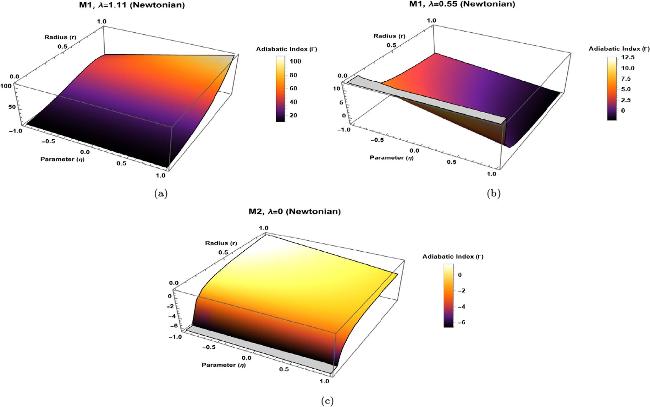
Figure 1. The schematic diagram shows (a) only stable behavior for the λ = 1.11 profile, (b) both stable and unstable behavior for the λ = 0.55 profile, and (c) only unstable behavior for the λ = 0 profile in the N domain, alongside different values of the correction parameter. |
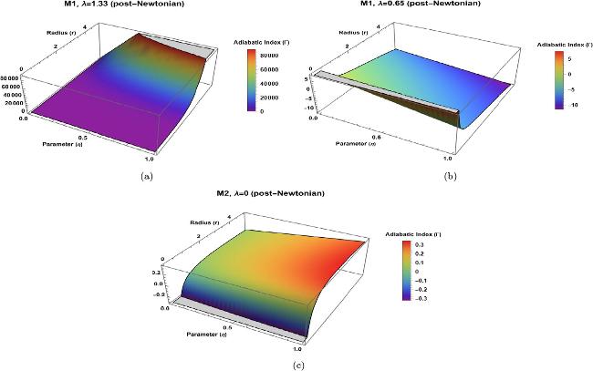
Figure 2. The schematic diagram shows (a) only stable behavior for the λ = 1.33 profile, (b) both stable and unstable behavior for the λ = 0.65 profile, and (c) only unstable behavior for the λ = 0 profile in the N domain, along with various other values of the correction parameter. |
4.8. Implications of stability analysis in the context of cosmic acceleration and dark energy models
In this study, we examined the dynamical instability of axially symmetric, anisotropic stellar configurations within the framework of the Starobinsky model with matter correction, i.e. f(R, T) gravity, described by f(R, T) = R + λR2 + ηT [96]. This formulation allows curvature matter coupling through the T term, giving rise to effective dark source components that can influence the internal structure and long term evolution of compact stars. Our perturbative approach, based on the adiabatic index Γ, identifies stability and instability regimes under N and pN limits. The onset of instability is shown to depend sensitively on the competition between gravitational attraction, repulsive curvature-induced effects, and anisotropic pressures, while the R2 term and the trace dependent contribution (via η) generate effective repulsive forces analogous to dark energy in large-scale cosmology.
The inclusion of anisotropic pressure components introduces additional degrees of freedom that extend the stability domain. Specifically, the curvature corrections in our model enhance outward-directed effective pressures, counteracting collapse in a manner reminiscent of negative-pressure dark energy effects. While our analysis focuses on local stability properties of compact, axially symmetric systems, the broader implication is that under certain parameter constraints such configurations may remain quasi-stable or completely evade collapse, mirroring the role of dark energy in driving accelerated cosmic expansion. Overall, our findings connect stellar scale stability with cosmological scale acceleration in two ways: (i) the effective dark source terms emerging from f(R, T) gravity act as additional energy-momentum components that can induce repulsive gravitational effects, potentially impacting the Universe’s expansion rate; (ii) the dependence of stability criteria on (λ, η) indicates a possible link between local instabilities and cosmic acceleration within a unified modified gravity framework, without requiring an explicit cosmological constant.
Thus, the curvature matter coupling inherent in f(R, T) gravity not only stabilizes compact objects but can also mimic dark energy behavior on cosmological scales. Future investigations may extend this framework by incorporating explicit couplings with dark energy models such as quintessence or phantom fields, or by generalizing to f(G), f(G, T), or higher-order f(R, T) theories, enabling a deeper understanding of the correspondence between local gravitational stability and large-scale accelerated expansion.
5. Conclusions
In this paper, we investigated the physical instability of a very limited group of celestial, axially symmetric fluid formations experiencing massive collapse in the setting of distinct two models of f(R, T) gravity. The complexity results from the existence of five different metric functions, which makes it easier to discard meridional and circulatory motions along the axis of symmetry. In the context of f(R, T) gravity, we calculated modified field equations for a self-gravitating system that continues to grow over an anisotropic environment. Due to this, some additional terms involve comparing the energy-momentum tensor trace to f(R) gravity, and a more comprehensive theory of GR is revealed. Observing the dynamical instability continuum using the perturbation methodology helped us deal with the complexity of the modified nonlinear partial differential equations. A particular formalism for f(R, T) gravity is examined, in addition to quadratic adjustments in both linear and Ricci scalar forms.
The perturbation approach separates static and non-static constituents of the revised equations of motion and continuity equations, proceeding to the formalism of a collapse equation. This involves perturbing the considered modified gravitational model; extra correction terms emerge because of modified gravitational theory impacts. We analyzed the behavior of collapsing, axially symmetric matter systems using a Harrison et al [107] EoS and non-conservation equations. Results clarified unstable conditions for N and pN eras, highlighting the crucial function of the Γ in dominance collapse behavior.
We highlighted the significance of our findings, compared them with existing literature, and discussed the broader implications and prospects of our work. We proposed a comparison of our results with relevant existing studies in the context of the dynamical instability of compact objects within f(R, T) gravity, which emphasizes how our findings align with or differ from previous works and their implications. We also explicitly discuss the significance of our results in terms of understanding the stability and collapse dynamics of axially symmetric stars, especially in the framework of alternative gravities. tTo provide a forward-looking perspective, we outline potential applications of our results to astrophysical phenomena and suggest different directions, such as the study of specific f(R, T) models under extreme astrophysical conditions or their connections to observational data. A comparison of results between f(R, T), f(R) gravity and GR highlights several distinct features and introduces new effects that arise due to the modifications in the underlying gravitational framework. In this study, we inspect the dynamical instability of axially symmetric structures across a peculiar f(R, T) gravity, which is expressed as: f(R, T) = R + λR2 + ηT, and f(R, T) = R + ηT, where λ and η are arbitrary parameters [96]. The impact of Γ during the N and pN eras is investigated in this inspection. The role of Γ is an important component of the metric that describes the thermodynamic features of a fluid structure, impacting the evolution and instability of dense astrophysical configurations. These findings are aligned with those outlined in [97, 108, 110] and account for the static components of the design. Consequently, one can observe that:
Curvature and a trace of the energy-momentum tensor induce effects as in f(R), and f(R, T) gravities; the Ricci scalar R and a trace of the energy-momentum tensor T are modified by additional terms introduced through the functional form of f(R) and f(R, T). These modifications lead to extra curvature contributions that are absent in GR. Specifically, the higher-order curvature terms λR2 or ηT corrections significantly influence the dynamics of the system, impacting the collapse conditions and the instability ranges. These effects are encapsulated in the form of dark source terms, which emerge as additional forces that modify the balance between gravitational and pressure forces.
In GR, the stability of a collapsing system is primarily governed by the interplay between gravitational attraction and pressure gradients, while in f(R) and f(R, T) gravities, the inclusion of curvature terms and the terms due to the trace of the energy-momentum tensor introduce modifications to the instability range. For instance, (i) the instability range in f(R) gravity is sensitive to the choice of the functional form of f(R), such as the Starobinsky model or logarithmic corrections. In the N and pN domain, the constraint will reduce to f(R) gravity by applying a standard limit like η → 0. Then our results will reduce to the Starobinsky model, i.e. f(R, T) = R + λR2, and will be well consistent with [108]. Furthemore, results for the instability of the axial system in f(R) gravity are compatible with [109]. (ii) The critical value of the Γ is altered due to the additional curvature terms, leading to new conditions for stability or instability, and similarly in the case of the presence of a trace of the energy-momentum tensor, f(R, T) functions.
The f(R) gravity or f(R, T) gravity introduce effective forces that arise from the modified field equations. These forces, which stem from the additional curvature terms in the case of f(R) functions, or from both the curvature and trace of the energy-momentum tensor in f(R, T) functions, can act as repulsive or attractive depending on the specific choice of f(R) or f(R, T). For instance, anti-gravitational effects are observed in certain cases, which can delay the onset of collapse or lead to different equilibrium configurations compared to GR in N and pN domains, as well as dark source terms contributing to anisotropic pressure, impacting the structure and evolution of compact objects.
The corrections in f(R) or f(R, T) gravities have some cosmological implications for the late-time evolution of the Universe, such as accelerated expansion, which are not captured by GR alone., However, for local systems such as compact stars, these corrections influence the stability and collapse dynamics in both N and pN eras.
The dynamics of specific parameters alter when comparing specific parameters in f(R), f(R, T) gravities with GR: the time scales for achieving hydrostatic equilibrium are modified due to the altered collapse equations in f(R) or f(R, T), whereas the density profile, pressure gradients, and energy flux behave differently in f(R) and f(R, T), introducing novel features such as oscillatory instabilities or delayed collapse. Our findings are compatible with [74, 97, 101, 108] and account for the static components of the configuration.
The minimally connected f(R, T) gravity introduces traits that minimize stability constraints, and inequalities for the Γ are established in equations (37 ), (38 ), (40 ), and (41 ) for our examined cosmic structures. To guarantee dynamical instability, the Γ needs to fulfill these specified requirements, which means that the cosmic formations can only display the stability spectrum if it deviates from these particular inequalities in N and pN eras. The hydrostatic equilibrium phases, which are linked by f(R, T) gravitational field equations that relate matter composition with gravity, are essential for the unstable behavior of compact matter.
Some new effects can be stated as follows. The modifications in f(R) gravity lead to the emergence of effects that are absent in GR. The additional curvature terms can stabilize certain compact configurations that would otherwise collapse or show unstable behavior in GR with N or pN approximation and modified gravitational radiation predictions due to the extra curvature contributions. There is a dependence of stability on higher-order derivatives of metric potentials and the chosen f(R) and f(R, T) theories.
We analyzed the dynamical behavior of anisotropic matter in f(R, T) gravity for both N and pN eras, with stability criteria derived from equations (37 ), (38 ), (40 ), and (41 ), in which stability is influenced by pressure anisotropy, energy density profiles, and correction parameter λ, and where different λ values yield varying stable and unstable behaviors as illustrated in figures 1 and 2. Hydrostatic equilibrium is achieved when the Γ satisfies the derived conditions, highlighting the interplay of fluid properties and extra curvature terms in determining stability.
Consequently, one can conclude that the features that appear in f(R) or f(R, T) theory, when compared to GR, include additional curvature effects, altered stability criteria, effective dark source forces, and new dynamical behavior and this effect can be observed through schematic diagrams established for our considered extremely limited class of axially symmetric, collapsing, self-gravitating fluid configuration. The instability holds for the highly limited group of axial symmetric celestial formations, which we investigated, assuming that all terms in the previous inequality are fulfilled for the GR case. In our exploration of minimally linked f(R, T) gravity functions, we established extra curvature properties that effect the stability limits. Our findings align with those of f(R) gravity when η = 0 which is consistent with [108] and with GR when η = 0 = λ, which is compatible with [112]. Our results demonstrate a close relationship between the stability of compact matter and the various stages of hydrostatic equilibrium. The gravitational field equations f(R, T) govern these equilibrium stages, which demonstrate a relationship between matter configuration and gravity. These modifications provide a richer framework for understanding the evolution of compact objects and offer insights into phenomena that may be attributed to modifications of gravity beyond GR.
Declarations: conflict of interest
The authors declare that they have no known competing financial interests or personal relationships that could have appeared to influence the work reported in this paper.
Appendices sections
We have condensed long and complicated expressions into more manageable forms to improve the readability and usability of our calculated expressions. The appendices sections of this publication contain full and extensive descriptions of these terms. With this method, we can still offer detailed calculations for reference while providing the important details in a more comprehensive form.
Appendix A
The extra curvature factors appear due to the revised theory of gravity in the modified field equations under consideration. These factors are labeled as ${\psi }_{ij}^{{}^{{\prime} }s}$ where; ij = 00, 01, 02, 11, 12, 22, 33, and these terms are known as dark source ingredients. The detailed expressions for ${\psi }_{ij}^{{}^{{\prime} }s}$ are provided as:
$\begin{eqnarray*}\begin{array}{l}{\psi }_{00}=\frac{1}{{H}^{2}}\left(\left(1+2\lambda R\right)^{\prime\prime} +\frac{{\left(1+2\lambda R\right)}^{\theta \theta }}{{r}^{2}}\right)\\ \,-\,\frac{2}{{A}^{2}}\left(\frac{\dot{H}}{H}{\left(1+2\lambda R\right)}^{.}-\frac{\dot{C}}{2C}{\left(1+2\lambda R\right)}^{.}\right)\\ \,+\,\frac{1}{{r}^{2}}\left(\frac{{C}^{\theta }}{{H}^{2}C}\right){\left(1+2\lambda R\right)}^{\theta }\\ \,+\,\frac{1}{H}\left(\frac{1}{Hr}\left(1+2\lambda R\right)^{\prime} +\frac{C^{\prime} }{HC}\left(1+2\lambda R\right)^{\prime} \right),\\ {\psi }_{01}=-\left(\frac{A^{\prime} }{A}{\left(1+2\lambda R\right)}^{.}+\frac{\dot{H}}{H}\left(1+2\lambda R\right)^{\prime} -\dot{\left(1+2\lambda R\right)}^{\prime} \right),\\ {\psi }_{02}=-\left(\frac{{A}^{\theta }}{A}{\left(1+2\lambda R\right)}^{.}+\frac{\dot{H}}{H}{\left(1+2\lambda R\right)}^{\theta }-{\dot{\left(1+2\lambda R\right)}}^{\theta }\right),\end{array}\end{eqnarray*}$
$\begin{eqnarray*}\begin{array}{l}{\psi }_{12}=\frac{1}{r{H}^{2}}\left({\left(1+2\lambda \right)}^{{}^{{\prime} }\theta }-\frac{{H}^{\theta }}{H}\left(1+2\lambda R\right)^{\prime} \right)\\ \,-\,\frac{1}{r{H}^{2}}\left(\frac{1}{r}{\left(1+2\lambda R\right)}^{\theta }+\frac{H^{\prime} }{H}{\left(1+2\lambda R\right)}^{\theta }\right),\\ {\psi }_{11}=\frac{1}{{A}^{2}}{\left(1+2\lambda R\right)}^{..}-\frac{1}{{r}^{2}{H}^{2}}{\left(1+2\lambda R\right)}^{\theta \theta }\\ \,-\,\frac{1}{{A}^{2}}\left(\frac{\dot{A}}{A}{\left(1+2\lambda R\right)}^{.}-\frac{\dot{H}}{H}{\left(1+2\lambda R\right)}^{.}+\frac{\dot{C}}{C}{\left(1+2\lambda R\right)}^{.}\right)\\ \,-\,\left(\frac{1}{r}\left(1+2\lambda R\right)^{\prime} \right.+\,\frac{A^{\prime} }{A}\left(1+2\lambda R\right)^{\prime} \\ \,\left.+\,\frac{H^{\prime} }{H}\left(1+2\lambda R\right)^{\prime} +\frac{C^{\prime} }{C}\left(1+2\lambda R\right)^{\prime} \right)\\ \,-\,\frac{1}{{r}^{2}}\left(\frac{{A}^{\theta }}{A}{\left(1+2\lambda R\right)}^{\theta }-\frac{{H}^{\theta }}{H}{\left(1+2\lambda R\right)}^{\theta }+\frac{{C}^{\theta }}{C}{\left(1+2\lambda R\right)}^{\theta }\right),\end{array}\end{eqnarray*}$
$\begin{eqnarray*}\begin{array}{l}{\psi }_{22}=\frac{1}{{A}^{2}}{\left(1+2\lambda R\right)}^{..}-\frac{1}{{H}^{2}}\left(1+2\lambda R\right)^{\prime\prime} +\,\frac{1}{{A}^{2}}\left(\frac{\dot{A}}{A}{\left(1+2\lambda R\right)}^{.}-\frac{\dot{H}}{H}{\left(1+2\lambda R\right)}^{.}-\frac{\dot{C}}{C}{\left(1+2\lambda R\right)}^{.}\right)\\ \,-\,\left(\frac{A^{\prime} }{A}\left(1+2\lambda R\right)^{\prime} \right.\left.\,-\,\frac{H^{\prime} }{H}\left(1+2\lambda R\right)^{\prime} -\frac{C^{\prime} }{C}\left(1+2\lambda R\right)^{\prime} \right)\frac{1}{{H}^{2}} & \,\end{array}\end{eqnarray*}$
$\begin{eqnarray*}\begin{array}{l}\,-\frac{1}{{r}^{2}{H}^{2}}\left(\frac{{A}^{\theta }}{A}\left(1+2\lambda R\right)^{\prime} +\frac{{H}^{\theta }}{H}\left(1+2\lambda R\right)^{\prime} \right.\left.\,+\,\frac{{C}^{\theta }}{C}\left(1+2\lambda R\right)^{\prime} \right),\\ \,{\psi }_{33}=\frac{1}{{A}^{2}}{\left(1+2\lambda R\right)}^{..}-\frac{1}{{H}^{2}}\left(\left(1+2\lambda R\right)^{\prime\prime} \right.+\,\left.\frac{1}{{r}^{2}}{\left(1+2\lambda R\right)}_{R}^{\theta \theta }\right)\\ \,+\,\frac{1}{{A}^{2}}\left(2\frac{\dot{H}}{H}{\left(1+2\lambda R\right)}^{.}-\frac{\dot{A}}{A}{\left(1+2\lambda R\right)}^{.}\right)-\,\frac{1}{{H}^{2}}\left(\frac{{A}^{{\prime} }}{A}\left(1+2\lambda R\right)^{\prime} +\frac{1}{r}\left(1+2\lambda R\right)^{\prime} \right)-\,\frac{1}{{r}^{2}}\left(\frac{{A}^{\theta }}{{H}^{2}A}\right){\left(1+2\lambda R\right)}^{\theta }.\end{array}\end{eqnarray*}$
The static portions of our known modified field equations (7 )–(11 ), are as follows:
$\begin{eqnarray*}\begin{array}{l}{\sigma }_{0}+{\psi }_{00}-\frac{1}{2}({R}_{0}+\lambda {R}_{0}^{2}+\eta {T}_{0})+\frac{1}{2}{R}_{0}\left(1+2\lambda {R}_{0}\right)=\,\frac{{A}_{0}^{4}\left(1+2\lambda {R}_{0}\right)}{{r}^{2}{H}_{0}}\\ \,\times \left[\frac{r(r{C}_{0}^{\prime\prime} +{C}_{0}^{{\prime} })+{C}_{0}^{\theta \theta }}{{C}_{0}}\right.\left.+\,\frac{r(r{H}_{0}^{\prime\prime} +{H}_{0}^{{\prime} })+{H}_{0}^{\theta \theta }}{{H}_{0}^{2}}+\frac{1}{{H}_{0}}\left\{-{r}^{2}{H}_{0}^{{}^{{\prime} }2}-\frac{{H}_{0}^{\theta 2}}{{H}_{0}^{2}}\right\}\right],\end{array}\end{eqnarray*}$
$\begin{eqnarray*}\begin{array}{l}{\psi }_{01}=0,\quad \quad {\psi }_{02}=0,\\ {\psi }_{12}+(1+\eta ){P}_{xy0}=r{H}_{0}^{2}\left(1+2\lambda {R}_{0}\right)\left[\left(\frac{{C}_{0}^{{}^{{\prime} }\theta }}{{C}_{0}}+\frac{{A}_{0}^{{}^{{\prime} }\theta }}{{A}_{0}}\right)\frac{1}{{H}_{0}}\left\{\left(\frac{A{{\prime} }_{0}}{{A}_{0}}+\frac{C{{\prime} }_{0}}{{C}_{0}}\right){H}_{0}^{\theta }\right.\right.-\,\left.\left.\left(\frac{{C}_{0}^{\theta }}{{C}_{0}}+\frac{{A}_{0}^{\theta }}{{A}_{0}}\right)H{{\prime} }_{0}\right\}-\frac{1}{r}\left(\frac{{C}_{0}^{\theta }}{{C}_{0}}+\frac{{A}_{0}^{\theta }}{{A}_{0}}\right)\right],\\ \eta {\sigma }_{0}+(1+\eta ){P}_{xx0}+\frac{{R}_{0}+\lambda {R}_{0}^{2}+\eta {T}_{0}}{2}-\,\frac{{R}_{0}}{2}\left(1+2\lambda {R}_{0}\right)+\,{\psi }_{11}=-{H}_{0}^{2}\left(1+2\lambda {R}_{0}\right)\\ \,\times \,\left[\frac{1}{{C}_{0}}\right.\left\{\left(\frac{{A}_{0}^{{\prime} }}{{A}_{0}}+\frac{1}{r}+\frac{{H}_{0}^{{\prime} }}{{H}_{0}}\right){C}_{0}^{{}^{{\prime} }\theta }+\left(\frac{{C}_{0}^{\theta \theta }}{{r}^{2}{C}_{0}^{\theta }}-\frac{{H}_{0}^{\theta }}{{H}_{0}}\right){C}_{0}^{\theta }\right\}+\,{\frac{1}{A}}_{0}\left\{\left(\frac{1}{r}+\frac{{H}_{0}^{{\prime} }}{{H}_{0}}\right)\right.{A}^{{\prime} }\left.\left.+\left(\frac{{A}_{0}^{\theta }}{{r}^{2}}-\frac{{H}_{0}^{\theta }}{{H}_{0}}+\frac{{C}_{0}^{\theta }}{{C}_{0}}\right){A}_{0}^{\theta }\right\}\right],\end{array}\end{eqnarray*}$
$\begin{eqnarray*}\begin{array}{l}\eta {\sigma }_{0}+(1+\eta ){P}_{yy0}+\frac{{R}_{0}+\lambda {R}_{0}^{2}+\eta {T}_{0}}{2}-\,\frac{{R}_{0}}{2}\left(1+2\lambda {R}_{0}\right)+{\psi }_{22}=-{r}^{4}{H}^{2}\left(1+2\lambda {R}_{0}\right)\\ \,\times \,\left[\frac{1}{{C}_{0}}\right.\left\{{C}_{0}^{{}^{{\prime\prime} }}+\left(\frac{{H}_{0}^{{\prime} }}{{H}_{0}}+\frac{{A}_{0}^{{\prime} }}{{A}_{0}}\right){C}_{0}^{{\prime} }\right\}+\frac{1}{{r}^{2}}\left\{\left(\frac{{H}_{0}^{\theta }}{{H}_{0}}+\frac{{A}_{0}^{\theta }}{{A}_{0}}\right)\frac{{C}_{0}^{\theta }}{{C}_{0}}\right\}+\,\left({r}^{2}{A}_{0}^{\prime\prime} -\right.\left.\left.\frac{{r}^{2}{H}_{0}^{{\prime} }}{{H}_{0}}+\frac{{H}_{0}^{\theta }}{{H}_{0}}\right)\frac{1}{{r}^{2}{A}_{0}}\right], & \,\end{array}\end{eqnarray*}$
$\begin{eqnarray*}\begin{array}{l}\eta {\sigma }_{0}+(1+\eta ){P}_{zz0}+\frac{{R}_{0}+\lambda {R}_{0}^{2}+\eta {T}_{0}}{2}-\,\frac{{R}_{0}}{2}\left(1+2\lambda {R}_{0}\right)+{\psi }_{33}=-\frac{{C}_{0}^{2}\left(1+2\lambda {R}_{0}\right)}{{H}_{0}^{2}}\\ \,\times \Space{0ex}{3ex}{0ex}[\left\{{A}_{0}^{\prime\prime} +\frac{1}{r}\left({A}_{0}^{{\prime} }+\frac{{A}_{0}^{\theta \theta }}{r}\right)\right\}\frac{1}{{A}_{0}}-\,\left.\left\{\frac{{H}_{0}^{2}}{{H}_{0}}-{C}_{0}^{2}H{{\prime\prime} }_{0}-\frac{1}{r}\left(H{{\prime} }_{0}+\frac{{H}_{0}^{\theta \theta }}{r}-\frac{{H}_{0}^{2\theta }}{{H}_{0}r}\right)\right\}\frac{1}{{H}_{0}}\right]. & \,\end{array}\end{eqnarray*}$
The calculations and basic presumptions are explained in detail, and we explain the methods by which the conclusions were obtained and how they relate to GR. The relevant terms are as follows:
$\begin{eqnarray*}\begin{array}{l}{\eta }_{1}=\frac{{H}_{0}^{-2}}{\left(1+2\lambda {R}_{0}\right)}\left[\left(\frac{{H}_{0}^{{\prime} }}{{H}_{0}}+\frac{\eta {H}_{0}^{{\prime} }}{{H}_{0}}+\frac{\eta {A}_{0}^{{\prime} }}{{A}_{0}}+\frac{{A}_{0}^{{\prime} }}{{A}_{0}}-2{F}_{1}\right.\right.\\ \,+\,\frac{1}{r}+\frac{\eta }{r}+\left.\frac{{C}_{0}^{{\prime} }}{{C}_{0}}+\frac{\eta {C}_{0}^{{\prime} }}{{C}_{0}}\right){P}_{xx0}+\,\frac{1}{r}(1+\eta ){P}_{xy0}^{\theta }-\frac{\acute{{C}_{0}}}{{C}_{0}}(1+\eta ){P}_{zz0}+\,\frac{1}{r}\left(\frac{2{H}_{0}^{\theta }}{{H}_{0}}+\frac{2\eta {H}_{0}^{\theta }}{{H}_{0}}+\frac{\eta {A}_{0}^{\theta }}{{A}_{0}}+\frac{{A}_{0}^{\theta }}{{A}_{0}}\right.\\ \left.\,-\,2\frac{{\left(1+2\lambda {R}_{0}\right)}^{\theta }}{\left(1+2\lambda {R}_{0}\right)}+\frac{{C}_{0}^{\theta }}{{C}_{0}}+\frac{\eta {C}_{0}^{\theta }}{{C}_{0}}\right){P}_{xy0}-\,\left(\frac{1}{r}+\frac{\eta }{r}+\frac{{H}_{0}^{{\prime} }}{{H}_{0}}+\frac{\eta {H}_{0}^{{\prime} }}{{H}_{0}}\right){P}_{yy0}+\frac{{F}_{1}}{2}\\ \,\times \,\left(\eta {T}_{0}^{{\prime} }+\left({R}_{0}+\lambda {R}_{0}^{2}\right)+\left({R}_{0}+\lambda {R}_{0}^{2}\right)\right.\left.\left.\,-\,{R}_{0}^{{\prime} }\left(1+2\lambda {R}_{0}\right)+\eta {T}_{0}{F}_{1}\right)\Space{0ex}{1.25ex}{0ex}\right]\\ \,-\,{\left\{\frac{{\psi }_{01}}{{A}_{0}^{2}{H}_{0}^{2}\left(1+2\lambda {R}_{0}\right)}\right\}}^{.}+\left\{\frac{{\psi }_{11}}{{H}_{0}^{2}\left(1+2\lambda {R}_{0}\right)}\right\}^{\prime} \,+\,{\left\{\frac{{\psi }_{12}}{{H}_{0}^{2}\left(1+2\lambda {R}_{0}\right)}\right\}}^{\theta }+\left(\frac{{H}_{0}^{\theta }}{{H}_{0}}+\frac{{C}_{0}^{\theta }}{4{C}_{0}}+\frac{{A}^{\theta }}{4{A}_{0}}\right)\\ \,\times \,\frac{4{\psi }_{12}}{{H}_{0}^{2}\left(1+2\lambda {R}_{0}\right)}-\frac{{C}_{0}^{{\prime} }{H}_{0}^{-2}{C}_{0}^{-1}{\psi }_{33}}{\left(1+2\lambda {R}_{0}\right)}+\frac{{A}_{0}^{{\prime} }{A}_{0}^{-1}{H}_{0}^{-1}{\psi }_{00}}{\left(1+2\lambda {R}_{0}\right)}+\,\left(\frac{{H}_{0}^{{\prime} }}{{H}_{0}}+\frac{{C}_{0}^{{\prime} }}{3{C}_{0}}+\frac{{A}_{0}^{{\prime} }}{3{A}_{0}}+\frac{1}{3r}\right)\frac{3{H}_{0}^{-2}{\psi }_{11}}{\left(1+2\lambda {R}_{0}\right)}\\ \,-\,\left(\frac{1}{r}+\frac{{H}_{0}^{{\prime} }}{{H}_{0}}\right)\frac{{\psi }_{22}}{{H}_{0}^{2}\left(1+2\lambda {R}_{0}\right)},{\eta }_{3}=-\frac{1}{2}\left(\frac{2Yb}{{H}_{0}}+{F}_{1}\right)\left({R}_{0}+\lambda {R}_{0}^{2}\right)+\frac{{R}_{0}}{2}\left(\frac{2Yb}{{H}_{0}}+{F}_{1}\right)\\ \,\times \,\left(1+2\lambda {R}_{0}\right)+\frac{Ye+2{R}_{0}Ye}{2}-\frac{Ye}{2}\left({R}_{0}+\lambda {R}_{0}^{2}\right)-\,\frac{{R}_{0}E}{2}.\end{array}\end{eqnarray*}$
Appendix B
To make the computations easier, the function β(r, θ) is presented. Its full expression, which reflects some of the system’s characteristics, is provided here:
$\begin{eqnarray*}\begin{array}{l}\beta (r,\theta )=-\frac{{R}_{0}b}{{H}_{0}}\frac{{A}_{0}^{2}}{\left(\frac{b}{{H}_{0}}-\frac{c}{{C}_{0}}\right)}-\,{A}_{0}^{2}\left[\frac{e}{2}-\frac{{A}_{0}^{{\prime} }}{{A}_{0}}\left\{\frac{{C}_{0}^{{\prime} }}{{C}_{0}}\left(\frac{{c}^{{\prime} }}{{H}_{0}^{2}{C}_{0}^{{\prime} }}-\frac{a}{{A}_{0}{H}_{0}^{2}}\right.\right.\right.+\,\left.\frac{{a}^{{\prime} }}{{H}_{0}^{2}{A}_{0}^{{\prime} }}-\frac{c}{{C}_{0}{B}_{0}^{2}}\right)-\left(\frac{{b}^{{\prime} }}{b}-\frac{{H}_{0}^{{\prime} }}{{H}_{0}}\right)\frac{b{H}_{0}^{{\prime} }}{{H}_{0}^{4}}\\ \,+\,\frac{{C}_{0}^{\prime\prime} }{{C}_{0}}\left\{\left(\frac{c}{{C}_{0}}-\frac{c^{\prime\prime} }{{C}_{0}^{\prime\prime} }\right)\frac{1}{{H}_{0}^{2}}\right\}+\frac{{H}_{0}^{\theta }}{{r}^{2}{H}_{0}}{\left\{\frac{b}{{H}_{0}}\right\}}^{\theta }\frac{1}{{H}_{0}}-\,\frac{{C}_{0}^{\theta \theta }}{{C}_{0}}\left\{\left(\frac{c}{2{C}_{0}}-\frac{{c}^{\theta \theta }}{2{C}_{0}^{\theta \theta }}\right)\frac{1}{{H}_{0}}\right\}-\,\frac{{A}_{0}^{\prime\prime} }{{A}_{0}}\left\{\left(\frac{a}{2{A}_{0}}-\frac{a^{\prime\prime} }{2A{{\prime\prime} }_{0}}\right)\frac{1}{{H}_{0}}\right\}\\ \,-\,\frac{H{{\prime\prime} }_{0}}{{H}_{0}}\left\{\left(\frac{b}{2{H}_{0}}-\frac{b^{\prime\prime} }{2H{{\prime\prime} }_{0}}\right)\frac{1}{{H}_{0}}\right\}-\,\frac{1}{{H}_{0}}\left\{\frac{{H}_{0}^{\theta \theta }}{{H}_{0}}\left(\frac{b}{2{H}_{0}}-\frac{{b}^{\theta \theta }}{2{H}_{0}^{\theta \theta }}\right)\right.-\,\left.\frac{{A}_{0}^{\theta \theta }}{{A}_{0}}\left(\frac{a}{2{A}_{0}}-\frac{{a}^{\theta \theta }}{2{A}_{0}^{\theta \theta }}\right)\right\}+\left\{\frac{{H}_{0}c+{C}_{0}b}{{H}_{0}{C}_{0}}-\frac{a}{{A}_{0}}\right\}^{\prime} \\ \,\times \,\frac{1}{2r{H}_{0}^{2}}+\frac{{A}_{0}^{\theta }}{{A}_{0}}\left\{\frac{{C}_{0}^{\theta }}{{C}_{0}}\left(\frac{{c}^{\theta }}{2{C}_{0}^{\theta }}+\frac{{a}^{\theta }}{2{A}_{0}^{\theta }}\left.-\frac{a}{2{A}_{0}}-\frac{c}{2{C}_{0}}\right)\frac{1}{{H}_{0}}\right\}\right\}\times \,\left.\frac{1}{\left(\frac{b}{{H}_{0}}-\frac{c}{{C}_{0}}\right)}\right].\end{array}\end{eqnarray*}$
Some very lengthy terms ${D}_{i}^{{}^{{\prime} }{\rm{s}}}$ can be found in non-static equations that do not involve conservation. Other curvature components, represented by D2N, appeared as a result of changed gravity in the N period. In the context of the N period, these factors function as dark source terms. Their complete formulations are as follows: $\begin{eqnarray*}\begin{array}{l}{D}_{2{\rm{N}}}=\frac{Y}{\left(1+2\lambda {R}_{0}\right)}\left[\left(\frac{2{F}_{1}E}{\left(1+2\lambda {R}_{0}\right)}-\frac{4Yb}{r}\right.\right.+\,\left.\left(1-\frac{1}{r}\right)\frac{E}{\left(1+2\lambda {R}_{0}\right)}\right){P}_{xx0}-{F}_{1}{\bar{P}}_{xx}\\ \,-\,\left(2Yb+\frac{E}{\left(1+2\lambda {R}_{0}\right)}\right){P}_{xx0}^{{\prime} }+\frac{\eta }{r}{\bar{P}}_{yy}+\,\left(\frac{2E{F}_{1}}{\left(1+2\lambda {R}_{0}\right)}-\frac{{E}^{\theta }}{\left(1+2\lambda {R}_{0}\right)}\right.\left.-\frac{Yb{E}^{\theta }}{\left(1+2\lambda {R}_{0}\right)}\right){P}_{xy0}\\ \,-\,\frac{{\left(1+2\lambda {R}_{0}\right)}^{\theta }}{r\left(1+2\lambda {R}_{0}\right)}{\bar{P}}_{xy}-\frac{1}{r}\left(2Yb+\frac{E}{\left(1+2\lambda {R}_{0}\right)}\right){P}_{xx0}^{\theta }+\,\frac{E}{\left(1+2\lambda {R}_{0}\right)}{P}_{zz0}+\frac{1}{2}{\left(Ye+2{R}_{0}Ye\right)}^{{\prime} }\\ \,+\,\frac{\left(Ye+2{R}_{0}Ye\right)}{2{F}_{1}^{-1}}+\frac{E\left({R}_{0}+\lambda {R}_{0}^{2}\right)}{2\left(1+2\lambda {R}_{0}\right)}-\,\frac{E{F}_{1}\left({R}_{0}+\lambda {R}_{0}^{2}\right)}{\left(1+2\lambda {R}_{0}\right)}-\frac{Y{e}^{{\prime} }}{2}\left(1+2\lambda {R}_{0}\right)\\ \left.\,-\,\frac{E{\left({R}_{0}+\lambda {R}_{0}^{2}\right)}^{{\prime} }}{2\left(1+2\lambda {R}_{0}\right)}\right]+\left(2Yb+\frac{E}{\left(1+2\lambda {R}_{0}\right)}\right){\left\{\frac{{\psi }_{01}}{\left(1+2\lambda {R}_{0}\right)}\right\}}^{.}\\ \,+\,\left\{\left(2Yb+2Ya+\frac{E}{\left(1+2\lambda {R}_{0}\right)}\right)\right.{\left.\frac{{\psi }_{01}}{\left(1+2\lambda {R}_{0}\right)}\right\}}^{.}-\,\left(2Yb+\frac{E}{\left(1+2\lambda {R}_{0}\right)}\right)\\ \,-\,\left\{\left(2Yb+\frac{E}{\left(1+2\lambda {R}_{0}\right)}\right)\right.{\left.\frac{{\psi }_{11}}{\left(1+2\lambda {R}_{0}\right)}\right\}}^{{\prime} }-\,\left\{\left(2Yb+\frac{E}{\left(1+2\lambda {R}_{0}\right)}\right)\right.{\left.\frac{{\psi }_{12}}{\left(1+2\lambda {R}_{0}\right)}\right\}}^{\theta }\\ \,-\,\left(2Yb+\frac{E}{\left(1+2\lambda {R}_{0}\right)}\right)-\left(4\dot{Y}b+\dot{Y}a+\frac{c}{r}\dot{Y}\right)\frac{{\psi }_{01}}{\left(1+2\lambda {R}_{0}\right)}\\ \,+\,\left(3Y{b}^{{\prime} }+Y{a}^{{\prime} }+\frac{Y{c}^{{\prime} }}{r}-\frac{Yc}{{r}^{2}}-\frac{8Yb}{r}-\frac{2E}{r\left(1+2\lambda {R}_{0}\right)}\right)\frac{{\psi }_{11}}{\left(1+2\lambda {R}_{0}\right)}+\left(4Y{b}^{\theta }+Y{a}^{\theta }+\frac{Y{c}^{\theta }}{r}\right)\frac{{\psi }_{12}}{\left(1+2\lambda {R}_{0}\right)}\\ \,-\,\left(rY{b}^{{\prime} }-4Yb-\frac{E}{\left(1+2\lambda {R}_{0}\right)}\right)\frac{{\psi }_{22}}{r\left(1+2\lambda {R}_{0}\right)}.\end{array}\end{eqnarray*}$
The non-static, part energy density profile in the N domain can be expressed as: $\begin{eqnarray*}\begin{array}{l}{\bar{\sigma }}_{N}=-\frac{1}{2}\left\{\left(\frac{c}{2r}+b\right){\sigma }_{0}+2b{P}_{xx0}-2b{R}_{0}\left(1+2\lambda {R}_{0}\right)\right.+\,\left.\frac{2c}{r}{P}_{zz0}+2b{P}_{yy0}+e\left(1+2\lambda {R}_{0}\right)+2{D}_{1}\right\}Y.\end{array}\end{eqnarray*}$
The detailed expressions for D1pN is provided as: $\begin{eqnarray*}\begin{array}{l}{D}_{1{\rm{p}}{\rm{N}}}=\frac{1}{\dot{Y}\left(1+2\lambda {R}_{0}\right)}\left[{\sigma }_{0}\dot{E}+\frac{1}{2}\left(\frac{\left({R}_{0}+\lambda {R}_{0}^{2}\right)\dot{E}}{\left(1+2\lambda {R}_{0}\right)}-\frac{d}{dt}\left(Ye+2{R}_{0}Ye\right)\right)\right.\\ \,+\,\frac{{m}_{0}}{{r}_{2}}\left(\frac{\left({R}_{0}+\lambda {R}_{0}^{2}\right)\dot{E}}{\left(1+2\lambda {R}_{0}\right)}-\frac{d}{dt}\left(Ye+2{R}_{0}Ye\right)\right)+\,\left(2\dot{Y}a+2\dot{Y}b+6\frac{\dot{Y}a{m}_{0}}{{r}_{2}}+\frac{2\dot{Y}c{m}_{0}}{r{r}_{2}}+\dot{Y}c\right){\psi }_{00}\\ \,-\,\left(\frac{4Ya}{r}-2\frac{Yb}{r}-\frac{Yc}{{r}^{2}}\right.+\frac{2}{E}r\left(1+2\lambda {R}_{0}\right)+\,\frac{4{m}_{0}E}{{r}^{2}\left(1+2\lambda {R}_{0}\right)}-3Ya^{\prime} -2\frac{{m}_{0}E}{r\left(1+2\lambda {R}_{0}\right)}\\ \,+\,3\frac{{m}_{0}E}{{r}^{2}\left(1+2\lambda {R}_{0}\right)}-9\frac{Ya{m}_{0}}{{r}_{2}^{2}}-4\frac{Y{m}_{0}}{{r}_{2}^{2}}-\,3\frac{Ya^{\prime} {m}_{0}}{{r}_{2}}+6\frac{Yb{m}_{0}}{{r}_{2}^{2}}+\frac{Yb{m}_{0}}{r{r}_{2}}+2\frac{Yb^{\prime} {m}_{0}}{{r}_{2}}+2\frac{Yb{m}_{0}}{{r}_{2}^{2}}\\ \left.\,-\,4\frac{Yb{m}_{0}}{r{r}_{2}}\right){\psi }_{01}-\left(3\frac{Y{a}^{\theta }}{{r}^{2}}+\frac{Y{c}^{\theta }}{{r}^{3}}-2\frac{Y{b}^{\theta }{m}_{0}}{{r}^{2}{r}_{2}}\right){\psi }_{01}+\,\dot{Y}b{\psi }_{11}+\frac{\dot{Y}b{\psi }_{11}}{{r}_{2}}+\dot{Y}b{\psi }_{22}+\,\frac{\dot{Y}b}{r}{\psi }_{22}+\frac{Yc}{r}{\psi }_{33}\left.+2\frac{Yc{m}_{0}}{r{r}_{2}}{\psi }_{33}\right]\\ \,-\,{\left\{\left(2Ya+\frac{E}{\left(1+2\lambda {R}_{0}\right)}-\frac{{m}_{0}E}{r\left(1+2\lambda {R}_{0}\right)}\right)\frac{{\psi }_{00}}{\left(1+2\lambda {R}_{0}\right)}\right\}}^{.}+\,\left(\frac{E}{\left(1+2\lambda {R}_{0}\right)}\right.\left.+2Ya-\frac{{m}_{0}E}{r\left(1+2\lambda {R}_{0}\right)}\right){\left\{\frac{{\psi }_{00}}{\left(1+2\lambda {R}_{0}\right)}\right\}}^{.}\\ \,+\,\left\{\left(2Ya+2\frac{{m}_{0}Ya}{{r}_{2}}+\frac{E}{\left(1+2\lambda {R}_{0}\right)}\right.\right.+\,\left.2Yb-2\frac{{m}_{0}Yb}{{r}_{2}}\right){\left.\frac{{\psi }_{01}}{\left(1+2\lambda {R}_{0}\right)}\right\}}^{{\prime} }\\ \,+\,\left(2Ya+2\frac{{m}_{0}Ya}{{r}_{2}}+\frac{E}{\left(1+2\lambda {R}_{0}\right)}\right){\left\{\frac{{\psi }_{01}}{\left(1+2\lambda {R}_{0}\right)}\right\}}^{{\prime} }+\left(2Ya+2\frac{{m}_{0}Ya}{{r}_{2}}+\frac{E}{\left(1+2\lambda {R}_{0}\right)}\right)\\ \,\times \,{\left\{\frac{{\psi }_{02}}{\left(1+2\lambda {R}_{0}\right)}\right\}}^{\theta }+{\left\{\left(2Ya+2\frac{{m}_{0}Ya}{{r}_{2}}\right)\frac{{\psi }_{02}}{\left(1+2\lambda {R}_{0}\right)}\right\}}^{\theta }.\end{array}\end{eqnarray*}$
The extra curvature factors that appear due to the modified gravity theory in the non-static part of the non-conservation equations under consideration are the factors that may be labeled as D2pN; these terms are known as dark source ingredients. The detailed expressions for D2pN are provided as: $ \begin{array}{l} D_{2 \mathrm{pN}}=\frac{1}{\left(1+2 \lambda R_{0}\right)}\left[\frac{m_{0} E}{r^{2}\left(1+2 \lambda R_{0}\right)} \sigma_{0}+\left(\frac{2 E F_{1}}{\left(1+2 \lambda R_{0}\right)}-\frac{4 m_{0} E F_{1}}{r\left(1+2 \lambda R_{0}\right)}+\frac{8 Y b m_{0}}{r}\right.\right. \\ \left.\quad-\frac{2 Y b m_{0}}{r^{2}}-\frac{2 E}{\left(1+2 \lambda R_{0}\right)}+\frac{2 m_{0} E}{r^{2}\left(2 \lambda R_{0}\right)}\right) P_{x x 0}-F_{1} \bar{P}_{x x}+\frac{2 m_{0} F_{1}}{r} \bar{P}_{x x} \\ \quad-\left(2 Y b-\frac{6 Y b m_{0}}{r_{2}}\left(1-\frac{2 m_{0}}{r}\right)\left(1+2 \lambda R_{0}\right)\right) P_{x x 0}^{\prime}+\frac{1}{r}\left(\frac{2 E F_{1}}{\left(1+2 \lambda R_{0}\right)}-\frac{4 m_{0} E F_{1}}{r\left(1+2 \lambda R_{0}\right)}-\frac{E^{\theta}}{\left(1+2 \lambda R_{0}\right)}+\frac{2 m_{0} E^{\theta}}{r\left(1+2 \lambda R_{0}\right)}\right. \\ \left.\quad-\frac{3 Y b\left(1+2 \lambda R_{0}\right)^{\theta}}{r\left(1+2 \lambda R_{0}\right)}-\frac{Y b\left(1+2 \lambda R_{0}\right)^{\theta}}{\left(1+2 \lambda R_{0}\right)}\right) P_{x y 0}-\left(\frac{\left(1+2 \lambda R_{0}\right)^{\theta}}{r\left(1+2 \lambda R_{0}\right)}-\frac{2 m_{0}\left(1+2 \lambda R_{0}\right)^{\theta}}{r^{2}\left(1+2 \lambda R_{0}\right)}\right) \bar{P}_{x y} \\ \quad-\frac{1}{r}\left(2 Y b-\frac{6 Y b m_{0}}{r}+\frac{E}{\left(1+2 \lambda R_{0}\right)}-\frac{2 m_{0} E}{r\left(1+2 \lambda R_{0}\right)}\right) P_{x x 0}^{\theta}-\left(\frac{E}{r\left(1+2 \lambda R_{0}\right)}-\frac{2 m_{0} E}{r^{2}\left(1+2 \lambda R_{0}\right)}-\frac{2 m_{0} E}{r^{2}\left(1+2 \lambda R_{0}\right)}\right) P_{y y 0} \\ \quad+\left(\frac{\eta}{r}-\frac{2 m_{0} \eta}{r r_{2}}\right) \bar{P}_{y y}+\left(\frac{2 m_{0} E}{r^{2}\left(1+2 \lambda R_{0}\right)}-\frac{E}{r\left(1+2 \lambda R_{0}\right)}\right) P_{z z 0}+\frac{1}{2}\left(\left(Y e+2 R_{0} Y e\right)^{\prime}\right. \\ \left.\quad+\frac{2\left(Y e+2 R_{0} Y e\right) E}{\left(1+2 \lambda R_{0}\right)}-\frac{\left(R_{0}+\lambda R_{0}^{2}\right) E F_{1}}{\left(1+2 \lambda R_{0}\right)}-2 R_{0}^{\prime} E+Y e^{\prime}-\frac{\left(R_{0}+\lambda R_{0}^{2}\right)^{\prime} E}{\left(1+2 \lambda R_{0}\right)}\right) \end{array}$
$\begin{eqnarray*}\begin{array}{l}\,-\,\left(\frac{Ya{m}_{0}}{{r}^{2}}-\frac{{m}_{0}E}{{r}^{2}\left(1+2\lambda {R}_{0}\right)}\right){\psi }_{00}-\,\dot{Y}\left(4b-\frac{4b{m}_{0}}{{r}_{2}}+a+\frac{a{m}_{0}}{{r}_{2}}+\frac{c}{r}\right){\psi }_{01}\\ \,+\,\left(3Yb^{\prime} -\frac{9Yb^{\prime} {m}_{0}}{{r}_{2}}+\frac{9Yb{m}_{0}}{{r}_{2}^{2}}+Ya+\frac{Ya{m}_{0}}{{r}_{2}}\right.-\,\frac{Ya{m}_{0}}{{r}_{2}^{2}}+\frac{Yc^{\prime} }{r}-\frac{2Yc^{\prime} {m}_{0}}{r{r}_{2}}-\frac{Yc}{{r}^{2}}+\frac{2Yc{m}_{0}}{{r}^{2}{r}_{2}}-\frac{2Yb}{r}\\ \,-\,\frac{2Yb{m}_{0}}{{r}_{2}^{2}}+\frac{4Yb{m}_{0}}{r{r}_{2}}-\frac{3E}{r\left(1+2\lambda {R}_{0}\right)}+\frac{3{m}_{0}E}{{r}^{2}\left(1+2\lambda {R}_{0}\right)}\left.+\,\frac{6{m}_{0}E}{{r}^{2}\left(1+2\lambda {R}_{0}\right)}\right){\psi }_{11}+\left(\frac{Yc^{\prime} }{r}\right.\left.-\frac{4Yc^{\prime} {m}_{0}}{r{r}_{2}}\right){\psi }_{12}\\ \,+\,\left(Yb^{\prime} -\frac{3Yb^{\prime} {m}_{0}}{{r}_{2}}-3Yb+\frac{12Yb{m}_{0}}{{r}_{2}}\right.-\,\frac{2Yb}{r}-\frac{E}{r\left(1+2\lambda {R}_{0}\right)}+\frac{2{m}_{0}E}{{r}^{2}\left(1+2\lambda {R}_{0}\right)}\\ \left.\,+\,\frac{{m}_{0}E}{{r}^{2}\left(1+2\lambda {R}_{0}\right)}\right){\psi }_{22}-\frac{1}{r}\left(\frac{Yc^{\prime} }{r}-\frac{2Yc^{\prime} {m}_{0}}{r{r}_{2}}-\frac{Yc}{r}-\frac{2Yc{m}_{0}}{r{r}_{2}}\right.-\,2Yb+\frac{Yb{m}_{0}}{{r}_{2}^{2}}-\frac{E}{r\left(1+2\lambda {R}_{0}\right)}\\ \left.\left.\,+\,\frac{2{m}_{0}E}{rr\left(1+2\lambda {R}_{0}\right)}\right){\psi }_{33}\right]+\left(2Yb-\frac{2Yb{m}_{0}}{{r}_{2}}+\frac{E}{\left(1+2\lambda {R}_{0}\right)}\right){\left\{\left(1+\frac{2{m}_{0}}{{r}_{2}}\frac{{\psi }_{01}}{\left(1+2\lambda {R}_{0}\right)}\right)\right\}}^{.}\\ \,-\,\left(\frac{E}{\left(1+2\lambda {R}_{0}\right)}\right.\left.+2Yb-\frac{2Yb{m}_{0}}{{r}_{2}}\right){\left\{\left(1+\frac{2{m}_{0}}{r}\frac{{\psi }_{11}}{\left(1+2\lambda {R}_{0}\right)}\right)\right\}}^{{\prime} }-\left(2Yb-\frac{2Yb{m}_{0}}{{r}_{2}}+\frac{E}{\left(1+2\lambda {R}_{0}\right)}\right){\left\{\left(1+\frac{2{m}_{0}{\psi }_{12}}{r\left(1+2\lambda {R}_{0}\right)}\right)\right\}}^{\theta } & \,\end{array}\end{eqnarray*}$
$\begin{eqnarray*}\begin{array}{l}+\,\left\{\left(2Yb-\frac{2Yb{m}_{0}}{{r}_{2}}+2Ya+\frac{2Y{m}_{0}}{{r}_{2}}\right.\right.+\,{\left.\left.\frac{\left(Ye+2{R}_{0}Ye\right)}{\left(1+2\lambda {R}_{0}\right)}\right)\frac{{\psi }_{01}}{\left(1+2\lambda {R}_{0}\right)}\right\}}^{.}\left\{\left(2Yb-\frac{2Yb{m}_{0}}{{r}_{2}}+\frac{E}{\left(1+2\lambda {R}_{0}\right)}\right.\right.\\ \left.-\,\frac{2{m}_{0}E}{\left(1+2\lambda {R}_{0}\right)}\right){\left.\frac{{\psi }_{11}}{\left(1+2\lambda {R}_{0}\right)}\right\}}^{{\prime} }+\,\left\{\left(2Yb-\frac{2Yb{m}_{0}}{{r}_{2}}+\frac{E}{\left(1+2\lambda {R}_{0}\right)}\right.\right.-\,\left.\frac{4Yb{m}_{0}}{r}-\frac{2{m}_{0}E}{\left(1+2\lambda {R}_{0}\right)}\right){\left.\frac{{\psi }_{12}}{\left(1+2\lambda {R}_{0}\right)}\right\}}^{\theta }. & \,\end{array}\end{eqnarray*}$