


1. Introduction
Spin-density separation, a defining feature of one-dimensional (1D) quantum many-body systems, emerges as the decoupling of low-energy collective excitations into independent spin and density modes, elegantly captured by the Tomonaga–Luttinger liquid framework for 1D Fermi gases [1–5]. Governed by tunable interactions, this phenomenon results in distinct linear dispersions for spin and density excitations, with velocities determined by Luttinger parameters and interaction strength [6–11]. Experimental techniques, such as Bragg spectroscopy [12, 13] and tunneling spectroscopy [14, 15], probe the dynamic structure factor (DSF) and tunneling conductance of 1D quantum systems, revealing distinct spectral features of spin and density excitations, which align with theoretical predictions and highlight the role of interaction strength in shaping excitation dynamics [16]. Although primarily observed in 1D Fermi systems, spin-density separation extends to 1D bosonic mixtures, suggesting its potential in higher-dimensional bosonic systems [17]. In a 1D bosonic gas, spin-charge separation enables the experimental observation of anyonic correlations, highlighting tunable statistical phases via strong interactions [18]. However, whether spin-density separation persists in higher-dimensional systems remains an important question, reflecting the critical role of dimensionality in modulating quantum correlations and collective phenomena.
Along this research line, spin-density separation in two-component bosonic mixtures in higher dimensions is confirmed to exist without relying on bosonization and is driven by distinct interaction types. In higher-dimensional bosonic mixtures, weakly interacting contact interactions govern the separation [19]. Meanwhile, P-wave interactions in three-dimensional (3D) bosonic mixtures modulate the separation dynamics, shaping a single degree-of-freedom peak observable in Bragg spectroscopy measurements [20]. Nevertheless, how interactions with more complex degrees of freedom—such as finite-range interactions—enable precise control of spin-density separation remains an important question. This reflects the critical role of complex interatomic interactions in shaping quantum correlations and collective phenomena, particularly through their influence on excitation spectra and mode-decoupling mechanisms.
Another important motivation for this work stems from the emergence of exotic many-body phenomena—including quantum droplets [21–23], phase separation [24–26], mixed bubble states [27, 28], and miscible–immiscible transitions [29–31]—in two-component bosonic mixtures. These phenomena are driven by the intricate interplay between interactions and quantum fluctuations. In the weakly interacting regime, they are predominantly governed by the competition between intra- and interspecies s-wave contact interactions, where the s-wave scattering length serves as the primary tunable parameter [32–34]. Beyond this standard paradigm, a diverse array of interactions—such as dipole-dipole interactions, Rabi coupling, spin–orbit coupling, and finite-range interactions—introduce additional degrees of freedom. These include non-locality, spin coherence, and momentum-dependent coupling, enabling precise sculpting of the effective interatomic potential [35–42]. Such interactions significantly expand the spectrum of accessible quantum phases. Crucially, finite-range interactions have recently emerged as a critically important control parameter [43–48]. In two-component systems, they play a pivotal role in stabilizing quantum droplets and modulating density profiles beyond the contact-interaction approximation [49, 50]. Furthermore, incorporating intra- and interspecies effective ranges (re, ${r}_{{\,\rm{e}\,}_{12}}$) facilitates independent control over both density and spin channels, enabling comprehensive interaction-driven modulation of collective excitations.
In this work, we employ effective field theory within the one-loop approximation to derive analytical expressions for a bosonic mixture subjected to finite-range interactions at zero temperature. For both 3D and 1D systems, we compute the ground-state energy, which recovers the results for homogeneous bosonic mixtures reported in [49], while the quantum depletion aligns with findings in [43, 51] in the limit of vanishing finite-range interactions. A primary focus of this work is the formulation of an effective action that governs the decoupled density and spin degrees of freedom, enabling the calculation of the corresponding DSFs. These reveal how finite-range interactions drive spin-density separation, a phenomenon amenable to experimental detection. Notably, this separation manifests distinct dimensional dependencies, with DSF peaks shifting to higher frequencies in 1D and lower frequencies in 3D as the interaction strength increases, underscoring the pivotal role of dimensionality. In the absence of finite-range interactions, our results converge with those of [19]. These findings provide deep insights into the influence of finite-range interactions on spin-density separation in quantum many-body systems across varying dimensions.
The paper is organized as follows. In section 2 , we develop a model for a two-component bosonic mixture in both the continuous 1D limit and 3D scenarios under finite-range interactions, utilizing an effective field theory approach. In section 3 , we derive analytical expressions for the ground-state energy and quantum depletion under finite-range interactions within the same theoretical framework. In section 4 , we explore the impact of finite-range interactions on spin-density separation across dimensions, examining the distinct behavior in 1D and 3D systems through DSFs. Section 5 summarizes our findings and outlines the experimental conditions necessary for observation of the proposed phenomena.
2. Functional integration of the D-dimensional bosonic mixtures
2.1. Partition function of the system
In this work, we are interested in a two-component weakly interacting bosonic mixture with finite-range interatomic interactions [49] in spatial dimensions (d = 1, 3), confined to a volume Ld. To analyze this system, we employ the path-integral formalism [20, 45, 46, 48], which naturally incorporates quantum fluctuations and enables systematic treatment of finite-range effects. The grand-canonical partition function of the system is then expressed as 1 ) reading $S\left[\bar{{\rm{\Psi }}},{\rm{\Psi }}\right]={\int }_{0}^{\hslash \beta }{\rm{d}}\tau {\int }_{{L}^{d}}{{\rm{d}}}^{d}{\boldsymbol{r}}\,{ \mathcal L }\left[\bar{{\rm{\Psi }}},{\rm{\Psi }}\right]$. The concrete expression of Lagrangian density ${ \mathcal L }\left[\bar{{\rm{\Psi }}},{\rm{\Psi }}\right]$ here takes the form 2 ), the ${\rm{\Psi }}\left({\boldsymbol{r}},\tau \right)={[{\psi }_{1},{\psi }_{2}]}^{{\rm{T}}}$ represent the two-component atomic bosonic complex fields, varying in both space r and imaginary time τ. The parameters μ and $\beta ={({k}_{\,\rm{B}\,}T)}^{-1}$ respectively define the thermodynamic chemical potential and the inverse thermal energy scale governing system equilibrium. The g(0) and ${g}_{12}^{(0)}$ denote the intra- and interspecies zero-range interatomic interaction coupling constants, respectively, with ${g}^{(0)}\ne {g}_{12}^{(0)}$ in view of the relevant experiment. Crucially, the higher-order terms g(2) and ${g}_{12}^{(2)}$ in equation (2 ) encode finite-range interaction effects through the s-wave pseudopotential expansion, where ${ \mathcal O }({k}^{2})$ momentum dependence induces beyond-mean-field correlations. The explicit forms of the interaction parameters g(0) and g(2) will be systematically derived in the subsequent analysis, establishing their competition as the microscopic origin of spin-density separation in the phase diagram.
$\begin{eqnarray}{ \mathcal Z }=\int { \mathcal D }\left[\bar{{\rm{\Psi }}},{\rm{\Psi }}\right]\exp \left\{-\frac{S\left[\bar{{\rm{\Psi }}},{\rm{\Psi }}\right]}{\hslash }\right\},\end{eqnarray}$
with the action functional in equation ( $\begin{eqnarray}\begin{array}{rcl}{ \mathcal L } & = & \displaystyle \sum _{i=1,2}\left\{{\psi }_{i}^{* }\left[\hslash {\partial }_{\tau }-\frac{{\hslash }^{2}}{2m}{{\rm{\nabla }}}^{2}-\mu \right]{\psi }_{i}\right.\\ & & +\left.\frac{{g}^{\left(0\right)}}{2}{\left|{\psi }_{i}\right|}^{2}-\frac{{g}^{\left(2\right)}}{2}{\left|{\psi }_{i}\right|}^{2}{{\rm{\nabla }}}^{2}{\left|{\psi }_{i}\right|}^{2}\right\}\\ & & +{g}_{12}^{\left(0\right)}{\left|{\psi }_{1}\right|}^{2}{\left|{\psi }_{2}\right|}^{2}-{g}_{12}^{\left(2\right)}{\left|{\psi }_{1}\right|}^{2}{{\rm{\nabla }}}^{2}{\left|{\psi }_{2}\right|}^{2}.\end{array}\end{eqnarray}$
In equation (Our goal is to unravel the non-trivial interplay between dimensional confinement quantified by spatial dimensionality d and the microscopic interaction structure encoded in contact g(0) and higher-order g(2) interaction parameters based on the Lagrangian density ${ \mathcal L }$ in equation (2 ), which orchestrates spin-density separation through emergent quantum fluctuations.
As a first step, we derive the explicit functional dependence of the interaction parameters g(0) and g(2) on spatial dimensionality d in equation (2 ). In 3D, the intra- and interspecies s-wave interaction strengths are defined as ${g}^{\left(0\right)}=4\pi {\hslash }^{2}a/m$ and ${g}_{12}^{\left(0\right)}=4\pi {\hslash }^{2}{a}_{12}/m$, respectively, with a and a12 being the s-wave scattering lengths and m being the atomic mass. The finite-range interaction strengths are ${g}^{\left(2\right)}=2\pi {\hslash }^{2}{a}^{2}{r}_{\,\rm{e}\,}/m$ and ${g}_{12}^{\left(2\right)}=2\pi {\hslash }^{2}{a}_{12}^{2}{r}_{{\,\rm{e}\,}_{12}}/m$ with re and ${r}_{{\,\rm{e}\,}_{12}}$ being the finite-range lengths. All discussions of 1D systems in this work refer to quasi-1D cases, realized through strong transverse confinement with frequency ω⊥ and length ${l}_{\perp }=\sqrt{\hslash /m{\omega }_{\perp }}$ [52]. The effective s-wave interaction strengths are
$\begin{eqnarray*}\begin{array}{rcl}{g}^{\left(0\right)\left(\,\rm{1D}\,\right)} & = & \frac{2{\hslash }^{2}{a}^{\left(\,\rm{1D}\,\right)}}{m{l}_{\perp }^{2}}\frac{1}{1-C{a}^{\left(\,\rm{1D}\,\right)}/{l}_{\perp }},\\ {g}_{12}^{\left(0\right)\left(\,\rm{1D}\,\right)} & = & \frac{2{\hslash }^{2}{a}_{12}^{\left(\,\rm{1D}\,\right)}}{m{l}_{\perp }^{2}}\frac{1}{1-C{a}_{12}^{\left(\,\rm{1D}\,\right)}/{l}_{\perp }},\end{array}\end{eqnarray*}$
where ${a}^{\left(\,\rm{1D}\,\right)}$ and ${a}_{12}^{\left(\,\rm{1D}\,\right)}$ are the effective 1D scattering lengths, and $C=-\zeta (1/2)/\sqrt{2}\simeq 1.0326$, with ζ(x) being the Riemann zeta function [53]. For strong confinement (${l}_{\perp }\gg {a}^{\left(\,\rm{1D}\,\right)},{a}_{12}^{\left(\,\rm{1D}\,\right)}$), these simplify to ${g}^{\left(0\right)\left(\,\rm{1D}\,\right)}\approx 2{\hslash }^{2}{a}^{\left(\,\rm{1D}\,\right)}/m{l}_{\perp }^{2}$ and ${g}_{12}^{\left(0\right)\left(\,\rm{1D}\,\right)}\approx 2{\hslash }^{2}{a}_{12}^{\left(\,\rm{1D}\,\right)}/m{l}_{\perp }^{2}$ [54]. The finite-range interaction strengths are assumed to be ${g}^{\left(2\right)\left(\rm{1D}\,\right)}=-{\hslash }^{2}{r}_{\,\rm{e}}^{\left(\,\rm{1D}\,\right)}/m$ and ${g}_{12}^{\left(2\right)\left(\rm{1D}\,\right)}=-{\hslash }^{2}{r}_{{\,\rm{e}}_{12}}^{\left(\,\rm{1D}\,\right)}/m$, where ${r}_{\,\rm{e}\,}^{\left(\,\rm{1D}\,\right)}$ and ${r}_{{\,\rm{e}\,}_{12}}^{\left(\,\rm{1D}\,\right)}$ are the intra- and interspecies s-wave effective 1D ranges.Next, we plan to take an experimental viewpoint to reformulate the Lagrangian density ${ \mathcal L }$ in equation (2 ) using density (nρ) and spin (nσ) fluctuations. The quantum fluctuations of these quantities of both nρ and nσ can be directly accessible in cold-atom experiments through Bragg spectroscopy measurements of the DSF. Defining ${n}_{\rho }=(| {\psi }_{1}{| }^{2}+| {\psi }_{2}{| }^{2})/\sqrt{2}$ and ${n}_{\sigma }=(| {\psi }_{1}{| }^{2}-| {\psi }_{2}{| }^{2})/\sqrt{2}$, we express ${ \mathcal L }$ in equation (2 ) in the following form 3 ), the contact couplings ${g}_{\rho }^{(0)}={g}^{(0)}+{g}_{12}^{(0)}$ and ${g}_{\sigma }^{(0)}={g}^{(0)}-{g}_{12}^{(0)}$ characterize density and spin waves, respectively; meanwhile, finite-range couplings, ${g}_{\rho }^{(2)}={g}^{(2)}+{g}_{12}^{(2)}$ and ${g}_{\sigma }^{(2)}={g}^{(2)}-{g}_{12}^{(2)}$, govern their beyond-contact counterparts.
$\begin{eqnarray}\begin{array}{rcl}{ \mathcal L } & = & \bar{{\rm{\Psi }}}\left(\hslash {\partial }_{\tau }-\frac{{\hslash }^{2}}{2m}{{\rm{\nabla }}}^{2}-\mu \right){\rm{\Psi }}+\frac{{g}_{\rho }^{\left(0\right)}}{2}{n}_{\rho }^{2}+\frac{{g}_{\sigma }^{\left(0\right)}}{2}{n}_{\sigma }^{2}\\ & & -\frac{{g}_{\rho }^{\left(2\right)}}{2}{n}_{\rho }{{\rm{\nabla }}}^{2}{n}_{\rho }-\frac{{g}_{\sigma }^{\left(2\right)}}{2}{n}_{\sigma }{{\rm{\nabla }}}^{2}{n}_{\sigma }.\end{array}\end{eqnarray}$
In equation (Now, we are ready to investigate the non-trivial interplay between dimensional confinement and the microscopic interaction structure by calculating the ground-state energy, quantum depletion, and the DSF. In this context, we limit ourselves to the case where intraspecies interactions are all repulsive (${g}^{\left(0\right)}\gt 0$, ${g}^{\left(2\right)}\gt 0$) and we work in the superfluid phase, where a U(1) gauge symmetry of each component is spontaneously broken [36]. Under this assumption, the complex fields in equation (3 ) can be expanded as ${\psi }_{i}\left({\boldsymbol{r}},\tau \right)=\sqrt{{n}_{0}}+{\eta }_{i}\left({\boldsymbol{r}},\tau \right)$, where ${n}_{0}=| {\psi }_{i}^{\left(0\right)}{| }^{2}$ represents the 3D condensate or 1D quasi-condensate density within the Bogoliubov approximation [51, 53], while ${\eta }_{i}^{* }\left({\boldsymbol{r}},\tau \right)$ and ${\eta }_{i}\left({\boldsymbol{r}},\tau \right)$ denote the fluctuation fields above the condensate. The mean-field plus Gaussian approximation is obtained by expanding equation (3 ) up to the second order in ${\eta }_{i}^{* }\left({\boldsymbol{r}},\tau \right)$ and ${\eta }_{i}\left({\boldsymbol{r}},\tau \right)$.
Finally, the grand potential corresponding to our model system is given by
$\begin{eqnarray}{\rm{\Omega }}\left(\mu ,\sqrt{{n}_{0}}\right)={{\rm{\Omega }}}_{0}\left(\mu ,\sqrt{{n}_{0}}\right)+{{\rm{\Omega }}}_{g}\left(\mu ,\sqrt{{n}_{0}}\right),\end{eqnarray}$
with ${{\rm{\Omega }}}_{0}/{L}^{d}=-2\mu {n}_{0}+{g}^{\left(0\right)}{n}_{0}^{2}+{g}_{12}^{\left(0\right)}{n}_{0}^{2}$ being the mean-field grand potential, while Ωg takes into account Gaussian fluctuations. Requiring $\sqrt{{n}_{0}}$ to describe the condensate (3D Bose-Einstein condensate or quasi-1D), we ensure vanishing linear fluctuation terms in the action, confirming that $\sqrt{{n}_{0}}$ minimizes the action. Minimizing Ω0 via $\partial {{\rm{\Omega }}}_{0}/\partial \sqrt{{n}_{0}}=0$ yields the chemical potential $\mu =({g}^{(0)}+{g}_{12}^{(0)}){n}_{0}$.2.2. Bogoliubov excitations
In section 2.1 , we presented the system’s action in equation (2 ), paying special attention to finite-range interaction effects in the two-component mixture characterized by the parameters of g(2). In section 2.2 , we plan to derive the excitation spectrum from the Gaussian action, as shown in equation (4 ). To diagonalize the quadratic terms in ηi, ${\eta }_{i}^{* }$ in equation (3 ), we Fourier transform and introduce Nambu space [55], yielding the desired quadratic form 5 ) 5 ), ${{\boldsymbol{G}}}_{{\boldsymbol{k}}n}^{-1}$, can be written as
$\begin{eqnarray}{S}_{2}\left[{\eta }_{1}^{* },{\eta }_{1},{\eta }_{2}^{* },{\eta }_{2}\right]=-\frac{\hslash }{2}\displaystyle \sum _{{\boldsymbol{k}}\ne 0,n}{{\boldsymbol{\Phi }}}_{{\boldsymbol{k}}n}{{\boldsymbol{G}}}_{{\boldsymbol{k}}n}^{-1}{{\boldsymbol{\Phi }}}_{{\boldsymbol{k}}n}^{\dagger },\end{eqnarray}$
where ℏk denotes the momentum and n labels the Matsubara frequencies with ωn = 2πn/ℏβ. The vector in equation ( $\begin{eqnarray*}{{\boldsymbol{\Phi }}}_{{\boldsymbol{k}}n}=\left({\eta }_{1{\boldsymbol{k}}n}^{* },{\eta }_{1-{\boldsymbol{k}}n},{\eta }_{2{\boldsymbol{k}}n}^{* },{\eta }_{2-{\boldsymbol{k}}n}\right),\end{eqnarray*}$
resides in the appropriate Nambu space, and the inverse Green’s function of the system in equation ( $\begin{eqnarray}-\hslash {{\boldsymbol{G}}}_{{\boldsymbol{k}}n}^{-1}=\beta \left(\begin{array}{cc}-\hslash {G}_{B{\boldsymbol{k}}n}^{-1} & \hslash {{\rm{\Sigma }}}_{12}\\ \hslash {{\rm{\Sigma }}}_{12} & -\hslash {G}_{B{\boldsymbol{k}}n}^{-1}\end{array}\right),\end{eqnarray}$
with ${G}_{B{\boldsymbol{k}}n}^{-1}$ and Σ12 being 2 × 2 submatrices. Henceforth, 2 × 2 matrices are denoted by uppercase letters, while 4 × 4 matrices are represented by bold uppercase letters.The diagonal submatrices in equation (6 ) are given by 6 ), representing the self-energy due to interspecies coupling, is expressed as $\hslash {{\rm{\Sigma }}}_{12}\,=\left({g}_{12}^{\left(0\right)}+{g}_{12}^{\left(2\right)}{k}^{2}\right){n}_{0}I$, where I is a 2 × 2 matrix with all elements equal to 1.
$\begin{eqnarray}-\hslash {G}_{B{\boldsymbol{k}}n}^{-1}=\left(\begin{array}{cc}-{\rm{i}}\hslash {\omega }_{n}+{\epsilon }_{k}^{0}+g^{\prime} {n}_{0}, & g^{\prime} {n}_{0},\\ g^{\prime} {n}_{0}, & {\rm{i}}\hslash {\omega }_{n}+{\epsilon }_{k}^{0}+g^{\prime} {n}_{0},\end{array}\right),\end{eqnarray}$
with ${\epsilon }_{k}^{0}={\hslash }^{2}{k}^{2}/2m$ and $g^{\prime} ={g}^{\left(0\right)}+{g}^{\left(2\right)}{k}^{2}$. The off-diagonal matrix in equation (Furthermore, we define the matrix M as the inverse Green’s function in equation (6 ) at ωn = 0: 8 ) with the help of the Cayley–Hamilton theorem (see equation (A4 ) in appendix A for the detailed derivation):
$\begin{eqnarray}{\boldsymbol{M}}=\left(\begin{array}{cccc}{\epsilon }_{k}^{0}+g^{\prime} {n}_{0} & g^{\prime} {n}_{0} & g{{\prime} }_{12}{n}_{0} & g{{\prime} }_{12}{n}_{0}\\ g^{\prime} {n}_{0} & {\epsilon }_{k}^{0}+g^{\prime} {n}_{0} & g{{\prime} }_{12}{n}_{0} & g{{\prime} }_{12}{n}_{0}\\ g{{\prime} }_{12}{n}_{0} & g{{\prime} }_{12}{n}_{0} & {\epsilon }_{k}^{0}+g^{\prime} {n}_{0} & g^{\prime} {n}_{0}\\ g{{\prime} }_{12}{n}_{0} & g{{\prime} }_{12}{n}_{0} & g^{\prime} {n}_{0} & {\epsilon }_{k}^{0}+g^{\prime} {n}_{0}\end{array}\right),\end{eqnarray}$
with $g{{\prime} }_{12}={g}_{12}^{\left(0\right)}+{g}_{12}^{\left(2\right)}{k}^{2}$. The Bogoliubov modes E± can be analytically obtained by letting $\det M=0$ in equation ( $\begin{eqnarray}{E}_{\pm }=\sqrt{\frac{{\rm{Tr}}[{\left({\boldsymbol{\kappa }}{\boldsymbol{M}}\right)}^{2}]}{4}\pm \sqrt{\frac{{\left[{\rm{Tr}}{\left({\boldsymbol{\kappa }}{\boldsymbol{M}}\right)}^{2}\right]}^{2}}{16}-\det \left({\boldsymbol{\kappa }}{\boldsymbol{M}}\right)}}.\end{eqnarray}$
The excitation energies of E± in equation (9 ) can be written into the dimensionless form as 10 ) represent finite-range-interaction-modified Bogoliubov modes with λ± = 1 + zρ(σ). Here, the finite-range coupling strength ${z}_{\rho (\sigma )}=4\,m{n}_{0}{g}_{\rho (\sigma )}^{\left(2\right)}/{\hslash }^{2}$ depends on the reduced couplings ${g}_{\rho (\sigma )}^{\left(2\right)}={g}^{\left(2\right)}\pm {g}_{12}^{\left(2\right)}$ in the density (ρ) and spin (σ) channels.
$\begin{eqnarray}{f}_{\pm }=\frac{{E}_{\pm }}{{g}^{\left(0\right)}{n}_{0}}=\sqrt{\frac{{\epsilon }_{k}^{0}}{{g}^{\left(0\right)}{n}_{0}}\left(\frac{{\epsilon }_{k}^{0}}{{g}^{\left(0\right)}{n}_{0}}{\lambda }_{\pm }+2\pm 2y\right)},\end{eqnarray}$
where $y={g}_{12}^{\left(0\right)}/{g}^{\left(0\right)}$ is the s-wave contact coupling ratio. The f± in equation (Figure 1 shows the excitation spectra f± versus dimensionless wave vector $k^{\prime} =\hslash k/\sqrt{2m{g}^{(0)}{n}_{0}}$ for various finite-range couplings zρ(σ). We have checked that equation (10 ) is simplified into [56] for vanishing of the finite-range interaction coupling constant zρ(σ) = 0. The competition between contact (y) and finite-range (z) interactions distinctly modifies the density and spin excitations in figures 1(a) and (b), respectively. In the phonon regime (k → 0):
$\begin{eqnarray*}{f}_{\pm }\approx \sqrt{{\epsilon }_{k}^{0}(2\pm 2y)/{g}^{(0)}{n}_{0}},\end{eqnarray*}$
showing negligible z-dependence, as evident in figures 1(a) and (b). Conversely, in the high-energy limit (k → ∞): $\begin{eqnarray*}{f}_{\pm }\approx \sqrt{{\lambda }_{\pm }}\,{\epsilon }_{k}^{0}/{g}^{(0)}{n}_{0},\end{eqnarray*}$
where finite-range interactions (z) dramatically modify both fluctuations, evident in the $k^{\prime} \gg 0$ regimes.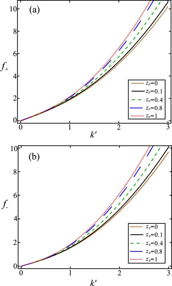
Figure 1. (a) The dimensionless excitation spectrum ${f}_{+}(k^{\prime} )$ from equation ( |
It is clear in figure 1 that the competition between the contact and finite-range interaction greatly affects both the density and spin quantum fluctuations of the model system, which directly determines the ground-state phase diagram of the model system. Hence, we are motivated to comprehensively summarize the ground-state phase diagram for bosonic systems across y and zρ(σ) in table 1.
Table 1. The ground-state phase diagram of bosonic systems in the y-zρ(σ) parameter space, where y denotes the contact coupling ratio and zρ(σ) is the finite-range interaction strength (negative/positive values correspond to attraction/repulsion). |
| Comp. | Parameters | Phase | References |
|---|---|---|---|
| Single | y = 0, zρ(σ) ≠ 0 | Finite-range EOS | [43–45, 47] |
| y = 0, zρ(σ) = 0 | Dimensional crossover | [57–59] | |
| y = 0, zρ(σ) > 0 | Finite-range dimensional crossover | [46, 48] | |
| | |||
| Spinor | y ≤ − 1, zρ(σ) = 0 | Quantum droplet | [23] |
| y ≤ − 1, zρ(σ) > 0 | Finite-range quantum droplet | [49, 50] | |
| 0 < y < 1, zρ(σ) = 0 | Spin-density separation | [19] | |
| 0 < y < 1, 0 ≤zρ(σ) ≤ 1 | Spin-density separation (finite-range) | This work | |
| y > 0, zρ(σ) = 0 | Mixed bubble phase | [27] | |
| y > 1, zρ(σ) = 0 | Phase separation | [60] | |
(ii) Two-component system (y ≠ 0):
We remark that our work together with the references in table 1 gives a complete description of how the contact and finite-range interaction couplings affect the ground-state phase diagram for both single-component and two-component weakly interacting bosonic systems.
3. Ground-state energy and quantum depletion in a d-dimensional system
In section 2 , we introduced the Lagrangian density of the system in equation (2 ) and derived the excitation spectrum in equation (9 ) within the framework of effective field theory. In section 3 , our goal is to derive explicit analytical expressions for the Lee–Huang–Yang (LHY) corrections to the ground-state energy and quantum depletion of d-dimensional bosonic mixtures under the one-loop approximation.
Our starting point is the grand potential of the Gaussian fluctuations ${{\rm{\Omega }}}_{g}\left(\mu ,\sqrt{{n}_{0}}\right)$ in equation (4 ), which is provided by
$\begin{eqnarray}{{\rm{\Omega }}}_{\,\rm{g}\,}\left(\mu ,\sqrt{{n}_{0}}\right)=\frac{1}{2}\displaystyle \sum _{{\boldsymbol{k}},\pm }\left[{E}_{\pm }+\frac{2}{\beta }{\mathrm{ln}}\left(1-{{\rm{e}}}^{-\beta {E}_{\pm }}\right)\right].\end{eqnarray}$
Next, our primary focus lies on the ground-state energy and quantum depletion of the model system at zero temperature.3.1. d = 3
In section 3.1 , we plan to investigate the ground-state energy and quantum depletion of the model system in 3D. To this end, we compute the ground-state energy of the model system, Eg = Ω0 + Ωg + 2L3μn0. Then, the expression for the ground-state energy can be written as follows:
$\begin{eqnarray}\begin{array}{l}\frac{{E}_{\,\rm{g}\,}}{{L}^{3}}={g}^{\left(0\right)}{n}_{0}^{2}+{g}_{12}^{\left(0\right)}{n}_{0}^{2}\\ +\,\frac{{g}^{\left(0\right)}{n}_{0}}{2{L}^{3}}\displaystyle \sum _{k^{\prime} \ne 0,\pm }\left\{{f}_{\pm }-\sqrt{{\lambda }_{\pm }}{k}^{{\prime} 2}-\frac{1\pm y}{\sqrt{{\lambda }_{\pm }}}+\frac{{\left(1\pm y\right)}^{2}}{2{\lambda }_{\pm }^{\frac{3}{2}}{k}^{{\prime} 2}}\right\},\end{array}\end{eqnarray}$
where $k^{\prime} =\hslash k/\sqrt{2m{g}^{\left(0\right)}{n}_{0}}$ represents the dimensionless wave vector.In equation (12 ), the first and second terms on the right-hand side represent the mean-field contribution, while all the subsequent terms correspond to the beyond-mean-field correction arising from quantum fluctuations. Notably, the final three terms in equation (12 ) are incorporated to eliminate power-law ultraviolet divergences in the momentum summation, a procedure effectively subsumed within a suitable renormalization of the coupling constants [61]. Rather than explicitly deriving the renormalized coupling constants, this subtraction yields a finite LHY correction, aligning with the physical goals of our study. The detailed derivation of these terms is presented in appendix B . In the continuum limit, the summation in equation (12 ) can be systematically replaced by an integral, leading to the analytical expression for the ground-state energy corresponding to equation (1 ) with d = 3 as follows 13 ) is consistent with the corresponding one in [49].
$\begin{eqnarray}\frac{{E}_{\,\rm{g}\,}}{{L}^{3}}={g}^{\left(0\right)}{n}_{0}^{2}+{g}_{12}^{\left(0\right)}{n}_{0}^{2}+\frac{{\left({g}^{\left(0\right)}{n}_{0}\right)}^{\frac{5}{2}}}{{(2\pi )}^{2}}{\left(\frac{2m}{{\hslash }^{2}}\right)}^{\frac{3}{2}}{h}_{\,\rm{3D}\,}\left({z}_{\rho ,\sigma }\right),\end{eqnarray}$
where the scaling function ${h}_{\,\rm{3D}\,}\left({z}_{\rho ,\sigma }\right)$ in terms of the variable zρ,σ can be solved analytically and the result reads $\begin{eqnarray}h\left({z}_{\rho ,\sigma }\right)=\frac{8\sqrt{2}{\left(1+y\right)}^{\frac{5}{2}}}{15{\left(1+{z}_{\rho }\right)}^{2}}+\frac{8\sqrt{2}{\left(1-y\right)}^{\frac{5}{2}}}{15{\left(1+{z}_{\sigma }\right)}^{2}}.\end{eqnarray}$
We remark that equation (For the coefficient y = 0.3, the corresponding results of equation (14 ) are illustrated in figure 2(a). In the absence of finite-range interactions, i.e. zρ(σ) = 0, the ground-state energy given by equation (12 ) simplifies to 16 ) accurately reproduces the relevant results in [23].
$\begin{eqnarray}\frac{{E}_{\,\rm{g}\,}^{(z=0)}}{{L}^{3}}={g}^{\left(0\right)}{n}_{0}^{2}+{g}_{12}^{\left(0\right)}{n}_{0}^{2}+\frac{{\left({g}^{\left(0\right)}{n}_{0}\right)}^{\frac{5}{2}}}{{\left(2\pi \right)}^{2}}{\left(\frac{2m}{{\hslash }^{2}}\right)}^{\frac{3}{2}}{h}^{\left(z=0\right)}\left(y\right),\end{eqnarray}$
where the function of ${h}_{\,\rm{3D}\,}^{\left(z=0\right)}\left(y\right)$ is given by $\begin{eqnarray}{h}^{\left(z=0\right)}\left(y\right)=\frac{8\sqrt{2}}{15}\left({\left(1+y\right)}^{\frac{5}{2}}+{(1-y)}^{\frac{5}{2}}\right),\end{eqnarray}$
and the expression in equation (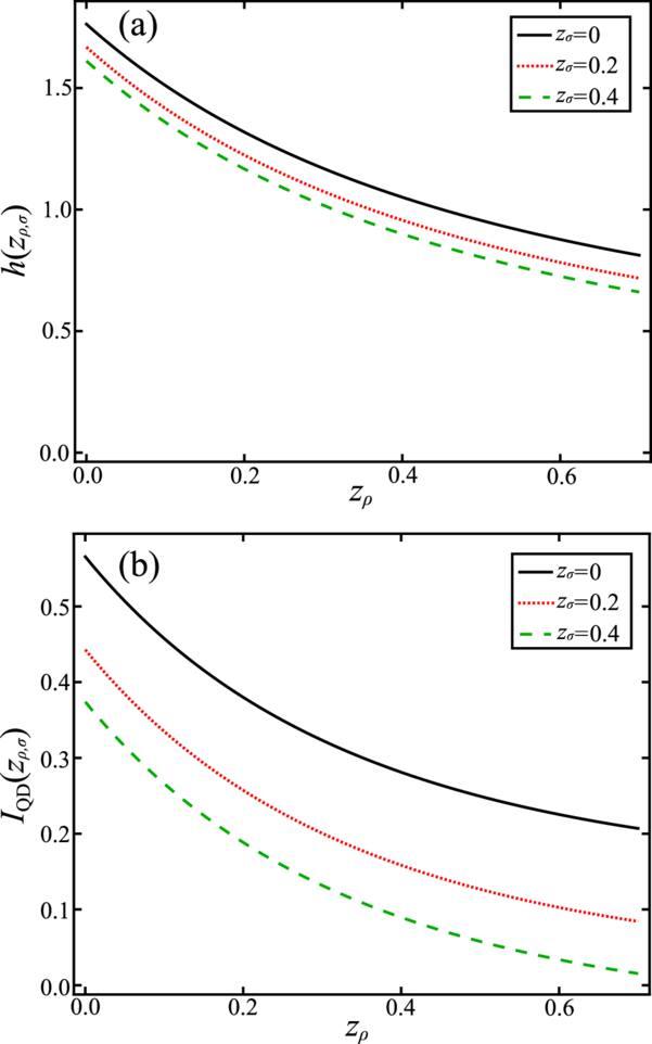
Figure 2. (a) The scaling function h(zρ) in equation ( |
We proceed to calculate the quantum depletion of our model system. The zero-temperature total particle number N can be derived from the zero-temperature grand potential Ω0 + Ωg using the thermodynamic formula $N=-\partial \left({{\rm{\Omega }}}_{0}+{{\rm{\Omega }}}_{g}\right)/\partial \mu $. Consequently, the quantum depletion ΔN = N − N0 of the system is obtained as
$\begin{eqnarray}\frac{{\rm{\Delta }}N}{N}=\frac{1}{{(2\pi )}^{2}}{\left(\frac{2m{g}^{\left(0\right)}}{{\hslash }^{2}}\right)}^{\frac{3}{2}}{\left({g}^{\left(0\right)}n\right)}^{\frac{1}{2}}{I}_{\,\rm{QD}\,}\left({z}_{\rho ,\sigma }\right),\end{eqnarray}$
where the scaling function ${I}_{\,\rm{QD}\,}\left(z\right)$ is defined as $\begin{eqnarray}\begin{array}{rcl}{I}_{\,\rm{QD}\,}\left({z}_{\rho ,\sigma }\right) & = & -\frac{\sqrt{2}\left({z}_{\sigma }-1\right){\left(1-y\right)}^{\frac{3}{2}}}{3{\left(1+{z}_{\sigma }\right)}^{2}}\\ \Space{0ex}{0.74em}{0ex} & & -\frac{\sqrt{2}{\left(y+1\right)}^{\frac{3}{2}}}{3\left(1+{z}_{\rho }\right)}+\frac{2\sqrt{2}{\left(y+1\right)}^{\frac{3}{2}}}{3{\left(1+{z}_{\rho }\right)}^{2}}.\end{array}\end{eqnarray}$
For the parameter y = 0.3, the corresponding results of equation (18 ) are illustrated in figure 2(b). To verify the correctness of these results, we consider the limit of vanishing finite-range interactions by setting zρ,σ = 0. In such a case, equation (17 ) can be rewritten into 19 ) is fully consistent with the corresponding results in [51].
$\begin{eqnarray}\frac{{\rm{\Delta }}N}{N}=\frac{1}{{(2\pi )}^{2}}{\left(\frac{2m{g}^{\left(0\right)}}{{\hslash }^{2}}\right)}^{\frac{3}{2}}{\left({g}^{\left(0\right)}n\right)}^{\frac{1}{2}}{I}_{\,\rm{QD}\,}^{(0)}\left(y\right),\end{eqnarray}$
with the scaling function ${I}_{\,\rm{QD}\,}^{(0)}\left(y\right)$ reading $\begin{eqnarray}{I}_{\,\rm{QD}\,}^{(0)}\left(y\right)=\frac{\sqrt{2}}{3}\left[\Space{0ex}{1.0ex}{0ex}{\left(1-y\right)}^{\frac{3}{2}}+{\left(y+1\right)}^{\frac{3}{2}}\Space{0ex}{1.0ex}{0ex}\right].\end{eqnarray}$
The analytical expression in equation (3.2. d = 1
For a quasi-1D system, the ground-state energy corresponding to equation (1 ) with d = 1 is expressed as: 21 ) are incorporated to mitigate ultraviolet divergences through a suitable renormalization of the coupling constants, as detailed in appendix B . In the continuum limit, the summation in equation (21 ) is replaced by an integral, yielding the analytical expression for the ground-state energy of the system, given by 23 ) aligns excellently with the corresponding one in [49]. When the parameter ${y}^{\left(\,\rm{1D}\,\right)}=0.3$, the corresponding results of equation (23 ) are presented in figure 3. At this point, we verify the accuracy of our results. In the limit where the finite-range interaction vanishes, the scaling function reduces to the following form
$\begin{eqnarray}\begin{array}{l}\frac{{E}_{\,\rm{g}\,}^{\left(\,\rm{1D}\,\right)}}{L}={g}^{\left(0\right)\left(\,\rm{1D}\,\right)}{n}_{0}^{2}+{g}_{12}^{\left(0\right)\left(\,\rm{1D}\,\right)}{n}_{0}^{2}+\frac{{g}^{\left(0\right)\left(\,\rm{1D}\,\right)}{n}_{0}}{2L}\\ \Space{0ex}{0.24em}{0ex}\,\times \,\displaystyle \sum _{{k}^{{\prime} \left(\,\rm{1D}\,\right)}\ne 0,\pm }\left\{{f}_{\pm }^{\left(\,\rm{1D}\,\right)}-\sqrt{{\lambda }_{\pm }^{\left(\,\rm{1D}\,\right)}}{({k}^{{\prime} \left(\,\rm{1D}\,\right))})}^{2}-\frac{1\pm {y}^{\left(\,\rm{1D}\,\right)}}{\sqrt{{\lambda }_{\pm }^{\left(\,\rm{1D}\,\right)}}}\right\},\end{array}\end{eqnarray}$
where ${k}^{{\prime} \left(\,\rm{1D}\,\right)}=\hslash k/\sqrt{2m{g}^{\left(0\right)\left(\,\rm{1D}\,\right)}{n}_{0}}$ denotes the dimensionless wave vector. The first two terms on the right-hand side correspond to the mean-field contribution, while the remaining terms account for beyond-mean-field corrections arising from quantum fluctuations. Notably, the final three terms in equation ( $\begin{eqnarray}\begin{array}{rcl}\frac{{E}_{\,\rm{g}\,}^{\left(\,\rm{1D}\,\right)}}{L} & = & {g}^{\left(0\right)\left(\,\rm{1D}\,\right)}{n}_{0}^{2}+{g}_{12}^{\left(0\right)\left(\,\rm{1D}\,\right)}{n}_{0}^{2}\\ & & -\frac{{\left({g}^{\left(0\right)\left(\,\rm{1D}\,\right)}{n}_{0}\right)}^{\frac{3}{2}}}{4\pi }{\left(\frac{2m}{{\hslash }^{2}}\right)}^{\frac{1}{2}}{h}^{\left(\,\rm{1D}\,\right)}\left({z}_{\rho ,\sigma }\right),\end{array}\end{eqnarray}$
where the scaling function ${h}_{\,\rm{1D}\,}\left({z}_{\rho ,\sigma }\right)$ is analytically determined as $\begin{eqnarray}{h}^{\left(\,\rm{1D}\,\right)}\left({z}_{\rho ,\sigma }\right)=\displaystyle \sum _{\pm }\frac{4\sqrt{2}}{3}\frac{{\left(1\pm {y}^{\left(\,\rm{1D}\,\right)}\right)}^{\frac{3}{2}}}{{\lambda }_{\pm }^{\left(\,\rm{1D}\,\right)}}.\end{eqnarray}$
The outcome in equation ( $\begin{eqnarray}{h}^{\left(0\right)\left(\,\rm{1D}\,\right)}=\displaystyle \sum _{\pm }\frac{4\sqrt{2}}{3}{\left(1\pm {y}^{\left(\,\rm{1D}\,\right)}\right)}^{\frac{3}{2}},\end{eqnarray}$
which is fully consistent with the results reported in [51]. For ${y}^{\left(\,\rm{1D}\,\right)}=0$, the system reduces to the single-component case, and the results remain consistent with those in [44]. In quasi-1D bosonic systems, the absence of true Bose–Einstein condensation in the thermodynamic limit, due to enhanced quantum fluctuations, precludes conventional quantum depletion, rendering this phenomenon characteristic of higher-dimensional condensates.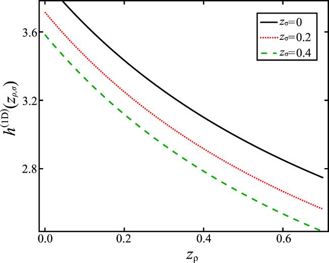
Figure 3. The dimensionless scaling function h(1D)(zρ, zσ) defined in equation ( |
Equations (13 ), (17 ), and (21 ) constitute a pivotal result of this study, delivering explicit analytical expressions for the LHY corrections to the ground-state energy and quantum depletion influenced by finite-range interactions in 3D and quasi-1D systems. The one-loop approximation captures leading-order quantum fluctuations, neglecting higher-order terms such as two-loop corrections, which are subdominant in the weakly interacting regime. This approach is controllable, as our results align with established limits (e.g. [49] for z = 0), thereby elucidating the impact of effective interaction strengths on the ground-state energy and quantum depletion and providing critical insights for precisely tuning the separation of the DSF with two degrees of freedom in section 4 .
4. Modulating spin-density separation via finite-range interaction
In section 3 , we derived the analytical expressions for the LHY corrections to the ground-state energy and quantum depletion of 1D and 3D bosonic mixtures, employing the one-loop approximation within the Bogoliubov framework. Building on these results, section 4 aims to elucidate the role of finite-range interactions in driving spin-density separation in a bosonic mixture. Our analysis covers both quasi-1D and 3D regimes, contrasting dimensionality effects. Crucially, we propose an experimental protocol to probe this phenomenon through the DSF, providing a direct path to validate our predictions with experimental signatures.
4.1. Density and spin excitation
In section 4.1 , our goal is to investigate how finite-range interactions can influence density and spin excitations in the system. For this purpose, we proceed to express the bosonic field ψi in terms of the number density ni and phase θi as ${\psi }_{i}=\sqrt{{n}_{i}}{{\rm{e}}}^{{\rm{i}}{\theta }_{i}}=\sqrt{{n}_{0}+\delta {n}_{i}}{{\rm{e}}}^{{\rm{i}}{\theta }_{i}}$, where n0 is the equilibrium density and δni denotes density fluctuations. To characterize spin-density separation, we transform to the basis $\delta {n}_{\rho (\sigma )}\,=(\delta {n}_{1}\pm \delta {n}_{2})/\sqrt{2}$ and ${\theta }_{\rho (\sigma )}=({\theta }_{1}\pm {\theta }_{2})/\sqrt{2}$, corresponding to the density (ρ) and spin (σ) degrees of freedom. Within this framework, the Gaussian-order action in equation (3 ) in real time is reformulated for a d-dimensional system (d = 1, 3) as follows: C . When zρ(σ) = 0, the effective action reduces to that of [19]. In equation (25 ), we emphasize that finite-range interactions, unlike other interaction types [19, 20], exclusively affect the kinetic term of density fluctuations in the Gaussian-order action, resulting in an effective mass correction. This decoupling ensures that finite-range effects only modify the number density fluctuation dynamics, without impacting the phase-related terms.
$\begin{eqnarray}\begin{array}{rcl}{S}_{\,\rm{g}\,} & = & \displaystyle \int {{\rm{d}}}^{d}{\boldsymbol{r}}\displaystyle \int {\rm{d}}t\displaystyle \sum _{\gamma =\rho ,\sigma }\left[\frac{{n}_{0}{\left({{\rm{\nabla }}}_{r}{\theta }_{\gamma }\right)}^{2}}{2m}+\delta {n}_{\gamma }{\partial }_{t}{\theta }_{\gamma }\right.\\ & & +\left.\frac{1}{2}\delta {n}_{\gamma }\left(\frac{{{\rm{\nabla }}}_{r}^{2}}{4{m}_{\gamma }{n}_{0}}+{g}_{\gamma }^{\left(0\right)}\right)\delta {n}_{\gamma }\right],\end{array}\end{eqnarray}$
with the coupling strength ${g}_{\rho \left(\sigma \right)}^{\left(0\right)}={g}^{\left(0\right)}\left(1\pm y\right)$. The reduced mass mρ(σ) = m/(1 + zρ(σ)) accounts for the effect of finite-range interactions, with the specific derivation of the finite-range action term provided in appendix By making a Fourier transformation, the action Sg in equation (25 ) can be rewritten as
$\begin{eqnarray}{S}_{g}\left(Q\right)={\boldsymbol{\Psi }}\left(Q\right){\boldsymbol{M}}^{\prime} {{\boldsymbol{\Psi }}}^{\dagger }\left(-Q\right),\end{eqnarray}$
where $Q=\left({\boldsymbol{k}},\omega \right)$ is a d + 1 vector denoting the momenta k and the frequency ω, and ${\boldsymbol{\Psi }}\left(Q\right)=\left(\delta {n}_{\rho },{\theta }_{\rho },\delta {n}_{\sigma },{\theta }_{\sigma }\right)$. Furthermore, the above matrix ${\boldsymbol{M}}^{\prime} $ can be deduced into $\begin{eqnarray}{\boldsymbol{M}}^{\prime} =\left(\begin{array}{cc}{M}_{\rho } & 0\\ 0 & {M}_{\sigma }\end{array}\right),\end{eqnarray}$
with the 2 × 2 submatrices $\begin{eqnarray}{M}_{\rho \left(\sigma \right)}=\left(\begin{array}{cc}\frac{{\hslash }^{2}{k}^{2}}{8{m}_{\rho \left(\sigma \right)}{n}_{0}}+\frac{{g}_{\rho \left(\sigma \right)}^{\left(0\right)}}{2} & \frac{1}{2}{\rm{i}}{\omega }_{\rho \left(\sigma \right)}\\ -\frac{1}{2}{\rm{i}}{\omega }_{\rho \left(\sigma \right)} & \frac{{\hslash }^{2}{k}^{2}{n}_{0}}{2m}\end{array}\right),\end{eqnarray}$
being the form of two submatrices, just the same as the one-component inverse Green function. Therefore, we can find that unlike 1D Fermi systems, which require bosonization to decouple spin and density degrees of freedom, the analysis here only necessitates consideration of fluctuations around the condensate density [19].With the help of equation (28 ), the analytical expressions of the density and spin excitation branches can be calculated as 29 ) is in exact agreement with that in equation (10 ), but is derived from the perspective of spin-density separation.
$\begin{eqnarray}{\varepsilon }_{\rho \left(\sigma \right)}\left(k\right)=\sqrt{\frac{{\hslash }^{2}{k}^{2}}{2m}\left(\frac{{\hslash }^{2}{k}^{2}}{2{m}_{\rho \left(\sigma \right)}}+2{g}_{\rho \left(\sigma \right)}^{\left(0\right)}{n}_{0}\right)},\end{eqnarray}$
where ${\varepsilon }_{\rho }\left(k\right)$ corresponds to the density mode and ${\varepsilon }_{\sigma }\left(k\right)$ corresponds to the spin mode. The excitation spectrum in equation (Using the excitation spectra in equation (29 ), we identify contributions to the ground-state energy from density (ρ) and spin (σ) degrees of freedom, denoted as Eρ and Eσ, respectively. These contributions are given by: 13 ) as it is expected.
$\begin{eqnarray}\frac{{E}_{\rho (\sigma )}}{{L}^{3}}={g}_{\rho }^{(0)}{n}_{0}^{2}+\frac{8{g}_{\rho (\sigma )}^{(0)\frac{5}{2}}{n}_{0}^{\frac{5}{2}}{m}^{\frac{3}{2}}}{15{\pi }^{2}{\hslash }^{3}{(1+{z}_{\rho (\sigma )})}^{2}}.\end{eqnarray}$
By simply adding Eρ and Eσ together and noting ${g}_{\rho }^{(0)}={g}^{(0)}+{g}_{12}^{(0)}$, the obtained ground-state energy of Eg = Eρ + Eσ can exactly recover the previous one in equation (4.2. Probing finite-range-induced spin-density separation by DSF
We now investigate how spin-density separation in a two-component bosonic mixture can be experimentally probed using Bragg spectroscopy. This technique involves inducing a density perturbation in the system while simultaneously probing both spin and density excitations. By utilizing two Bragg laser beams with momenta k1 and k2 and precisely tuning their frequency difference ω (kept significantly smaller than their detuning from the atomic resonance), it is possible to selectively excite density and spin waves within the Bose gas. Next, we plan to calculate the DSF of finite-range bosonic mixtures in 1D and 3D cases, respectively.
4.2.1. Density and spin DSF in 3D
To quantitatively analyze density and spin excitations, we are motivated to calculate the corresponding DSFs directly by following the method in [19], 31 ), the ${\chi }_{\rho \left(\sigma \right)}$, ${v}_{\rho \left(\sigma \right)}$ and Γ are referred to as the compressibility, sound speed, and damping rate, respectively. In the following, we plan to calculate these quantities one by one.
$\begin{eqnarray}{S}_{\rho \left(\sigma \right)}\left(k,\omega \right)\approx \frac{{\chi }_{\rho \left(\sigma \right)}{v}_{\rho \left(\sigma \right)}k{{\rm{\Gamma }}}_{\rho \left(\sigma \right)}}{2\left[{\left(\omega -{v}_{\rho \left(\sigma \right)}k\right)}^{2}+{{\rm{\Gamma }}}_{\rho \left(\sigma \right)}^{2}\right]}.\end{eqnarray}$
In equation (First, the compressibility ${\chi }_{\rho \left(\sigma \right)}$ in equation (31 ) can be directly calculated by the ground-state energy E through the expression ${\chi }^{-1}=\frac{1}{V}\frac{{\partial }^{2}E}{\partial {n}^{2}}$. Here, V represents the constant system volume and n = N/V denotes the density. By plugging equation (30 ) into the above definition of compressibility, the inverse compressibility related to density (ρ) and spin (σ) degrees of freedom can be directly calculated as
$\begin{eqnarray}\begin{array}{rcl}{\chi }_{\rho \left(\sigma \right)}^{-1} & = & \frac{16{g}_{\rho \left(\sigma \right)}^{\left(0\right)\frac{5}{2}}{m}^{\frac{3}{2}}{n}_{0}^{\frac{1}{2}}{z}_{\rho \left(\sigma \right)}^{2}}{5{\pi }^{2}{\hslash }^{3}{({z}_{\rho \left(\sigma \right)}+1)}^{4}}-\frac{16{g}_{\rho \left(\sigma \right)}^{\left(0\right)\frac{5}{2}}{m}^{\frac{3}{2}}{n}_{0}^{\frac{1}{2}}{z}_{\rho \left(\sigma \right)}}{3{\pi }^{2}{\hslash }^{3}{({z}_{\rho \left(\sigma \right)}+1)}^{3}}\\ \Space{0ex}{0.24em}{0ex} & & +\frac{2{g}_{\rho \left(\sigma \right)}^{\left(0\right)\frac{5}{2}}{m}^{\frac{3}{2}}{n}_{0}^{\frac{1}{2}}}{{\pi }^{2}{\hslash }^{3}{({z}_{\rho \left(\sigma \right)}+1)}^{2}}+{g}_{\rho }^{\left(0\right)}.\end{array}\end{eqnarray}$
Next, the sound velocity in equation (31 ) is defined as $v={\left(\frac{V}{mn}\frac{{\partial }^{2}E}{\partial {V}^{2}}\right)}^{1/2}$ at a constant particle number N. By plugging equation (30 ) into the above definition of sound velocity, its analytical expression related to density (ρ) and spin (σ) degrees of freedom can be deduced as
$\begin{eqnarray}\begin{array}{rcl}{v}_{\rho \left(\sigma \right)} & = & \left[\frac{16{g}_{\rho \left(\sigma \right)}^{\left(0\right)\frac{5}{2}}{m}^{\frac{1}{2}}{n}_{0}^{\frac{3}{2}}{z}_{\rho \left(\sigma \right)}^{2}}{5{\pi }^{2}{\hslash }^{3}{\left({z}_{\rho \left(\sigma \right)}+1\right)}^{4}}+\frac{2{g}_{\rho \left(\sigma \right)}^{\left(0\right)\frac{5}{2}}{m}^{\frac{1}{2}}{n}_{0}^{\frac{3}{2}}}{{\pi }^{2}{\hslash }^{3}{\left({z}_{\rho \left(\sigma \right)}+1\right)}^{2}}\right.\\ & & {\left.-\frac{16{g}_{\rho \left(\sigma \right)}^{\left(0\right)\frac{5}{2}}{m}^{\frac{1}{2}}{n}_{0}^{\frac{3}{2}}{z}_{\rho \left(\sigma \right)}}{3{\pi }^{2}{\hslash }^{3}{\left({z}_{\rho \left(\sigma \right)}+1\right)}^{3}}+\frac{{g}_{\rho }^{\left(0\right)}{n}_{0}}{m}\right]}^{\frac{1}{2}}.\end{array}\end{eqnarray}$
Before proceeding further, we would like to double-check the validity of equations (32 ) and (33 ) by seeing whether they can recover the well-known results in the limit case of the vanishing finite-range interactions zρ(σ) = 0. In this limit, the compressibility in equation (32 ) simplifies to 33 ) simplifies to
$\begin{eqnarray}{\chi }_{\rho \left(\sigma \right)}^{\left(0\right)}={g}_{\rho }^{\left(0\right)}+\frac{2{g}_{\rho \left(\sigma \right)}^{\left(0\right)\frac{5}{2}}{m}^{\frac{3}{2}}{n}_{0}^{\frac{1}{2}}}{{\pi }^{2}{\hslash }^{3}},\end{eqnarray}$
and the sound velocity in equation ( $\begin{eqnarray}{v}_{\rho \left(\sigma \right)}^{\left(0\right)}={\left[\frac{{g}_{\rho }^{\left(0\right)}{n}_{0}}{m}+\frac{2{g}_{\rho \left(\sigma \right)}^{\left(0\right)\frac{5}{2}}{m}^{\frac{1}{2}}{n}_{0}^{\frac{3}{2}}}{{\pi }^{2}{\hslash }^{3}}\right]}^{\frac{1}{2}},\end{eqnarray}$
consistent with the results for a contact-interaction s-wave bosonic mixture reported in [19]. These findings affirm the robustness of our theoretical framework, accurately capturing the transition from finite-range to contact interactions while maintaining the spin-density separation observed in the DSF.Finally, to evaluate the damping rate Γ for the DSF of a 3D two-component bosonic mixture with finite-range interactions, we employ the Beliaev damping framework developed for a single-component s-wave Bose gas, as detailed in [19]. Our calculations reveal that finite-range interactions solely influence the quadratic terms without affecting the damping mechanism. As a result, both the density and spin modes are governed by the bare mass m. The damping rate is thus expressed as Γ = 3ℏk5/(640πmn0), reflecting low-energy quasiparticle scattering in 3D systems, consistent with [19, 62]. This k5-dependent damping broadens the DSF peaks without altering the energy separation between the density and spin modes, as defined by the excitation spectra ϵρ and ϵσ in equation (29 ). Using these damping rates, we reformulate the DSFs as
$\begin{eqnarray}{S}_{\rho \left(\sigma \right)}={\chi }_{\rho \rm{}\,\rm{}\,}^{\left(0\right)}{J}_{\rho \left(\sigma \right)}\left(\omega ^{\prime} \right),\end{eqnarray}$
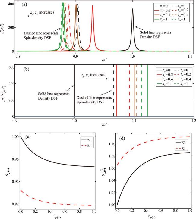
where the 3D dimensionless DSF functions or the density and spin degrees of freedom, ${J}_{\rho \left(\sigma \right)}\left(\omega ^{\prime} \right)$, are given by $\begin{eqnarray}{J}_{\rho \left(\sigma \right)}\left(\omega ^{\prime} \right)=\frac{{\zeta }_{\rho \left(\sigma \right)}{\alpha }_{\rho \left(\sigma \right)}{\rm{\Gamma }}/{v}_{\rho }^{\left(0\right)}k^{\prime} }{{(\omega ^{\prime} -{\alpha }_{\rho \left(\sigma \right)})}^{2}+{\left({\rm{\Gamma }}/{v}_{\rho }^{\left(0\right)}k^{\prime} \right)}^{2}}.\end{eqnarray}$
In equation (37 ), the dimensionless coefficients are defined as ${\alpha }_{\rho \left(\sigma \right)}={v}_{\rho \left(\sigma \right)}/{v}_{\rho ,\,\rm{3D}\,}^{\left(0\right)}$ and ${\zeta }_{\rho \left(\sigma \right)}={\chi }_{\rho }^{\left(0\right)-1}/{\chi }_{\rho \left(\sigma \right)}^{-1}$, with the dependence of αρ(σ) on the interaction parameters zρ(σ) depicted in figure 4(c). The momentum k is rendered dimensionless, as outlined in section 2 , where $k^{\prime} =\hslash k/\sqrt{2g{n}_{0}m}$, with $\hslash /\sqrt{2g{n}_{0}m}=1$. Consequently, the dimensionless frequency is given by $\omega ^{\prime} =\omega /{v}_{\rho }^{\left(0\right)}k^{\prime} $. For $k^{\prime} =1.25$ and y = 0.3, the density compressibility ${\chi }_{\rho \rm{}\,\rm{}\,}^{\left(0\right)}$ can be approximated as constant. The dimensionless DSF functions ${J}_{\rho (\sigma )}(\omega ^{\prime} )$ vary with frequency $\omega ^{\prime} $ for different values of the interaction parameters zρ and zσ, as illustrated in figure 4(a). In figure 4(a), we observe that the DSF peaks for both density and spin modes shift toward lower frequencies with increasing finite-range interaction strength, indicating enhanced interaction effects. The density wave exhibits a broader peak due to stronger Beliaev damping, whereas the spin wave retains a narrower and sharper response, underscoring their distinct dynamic behavior in 3D bosonic mixtures.
Figure 4. (a) The 3D dimensionless DSFs ${J}_{\rho }({\omega }^{{\prime} })$ and ${J}_{\sigma }({\omega }^{{\prime} })$ in equation ( |
4.2.2. Density and spin DSF in 1D
Having analyzed spin-density separation in 3D bosonic mixtures through DSFs, we now investigate the quasi-1D case to further elucidate this phenomenon. Following [19], the formal expression of the DSFs in 1D is given by
$\begin{eqnarray}{S}_{\rho (\sigma )}^{\,\rm{1D}\,}\left(k,\omega \right)=\,\rm{Im}\,\frac{{\chi }_{\rho \left(\sigma \right)}^{\left(\,\rm{1D}\,\right)}{v}_{\rho \left(\sigma \right)}^{\left(\,\rm{1D}\,\right)2}{k}^{2}}{{\omega }^{2}-{\omega }_{\rho \left(\sigma \right)}^{2}\left(k\right)},\end{eqnarray}$
with χρ(σ),1D representing the compressibility, ${v}_{\rho \left(\sigma \right)}^{\left(\,\rm{1D}\,\right)}$ being the sound velocity, and ${\omega }_{\rho \left(\sigma \right)}$ labelling the density and spin excitations. Next, we plan to obtain the analytical expressions of these three quantities.As a first step, the compressibility of χρ(σ),1D is determined by ${\chi }^{-1}=\frac{1}{L}\frac{{\partial }^{2}E}{\partial {n}^{2}}$ at constant system length L. We need to calculate the contribution to the ground-state energy of the density and spin excitations provided in equation (29 ), which are given as
$\begin{eqnarray}\frac{{E}_{\rho \left(\sigma \right)}^{\left(\,\rm{1D}\,\right)}}{L}=\frac{{g}_{\rho }^{\left(0\right)\left(\,\rm{1D}\,\right)}{n}_{0}^{2}}{2}-\frac{2}{3\pi }{\left(\frac{m}{{\hslash }^{2}}\right)}^{\frac{1}{2}}\frac{{\left({g}_{\rho \left(\sigma \right)}^{\left(0\right)\left(\,\rm{1D}\,\right)}{n}_{0}\right)}^{\frac{3}{2}}}{\left(1+{z}_{\rho \left(\sigma \right)}\right)}.\end{eqnarray}$
The above results agree with the corresponding results in [63], and in the limit zρ(σ) = 0 can reduce to the well-known Lieb–Liniger solution [64]. We proceed to calculate the inverse compressibility χ−1 induced by the density and spin excitations as $\begin{eqnarray}\begin{array}{rcl}{\chi }_{\rho \left(\sigma \right)}^{\left(\,\rm{1D}\,\right)-1} & = & -\frac{4{g}_{\rho \left(\sigma \right)}^{\left(0\right)\left(\,\rm{1D}\,\right)\frac{3}{2}}{m}^{\frac{1}{2}}{z}_{\rho \left(\sigma \right)}^{2}}{3\pi {n}_{0}^{\frac{1}{2}}{\left({z}_{\rho \left(\sigma \right)}+1\right)}^{3}}+\frac{2{g}_{\rho \left(\sigma \right)}^{\left(0\right)\left(\,\rm{1D}\,\right)\frac{3}{2}}{m}^{\frac{1}{2}}{z}_{\rho \left(\sigma \right)}}{\pi {n}_{0}^{\frac{1}{2}}\left({z}_{\rho \left(\sigma \right)}+1\right)}\\ & & -\frac{{g}_{\rho \left(\sigma \right)}^{\left(0\right)\left(\,\rm{1D}\,\right)\frac{3}{2}}{m}^{\frac{1}{2}}}{2\pi {n}_{0}^{\frac{1}{2}}\left({z}_{\rho \left(\sigma \right)}+1\right)}+{g}_{\rho }^{\left(0\right)\left(\,\rm{1D}\,\right)}.\end{array}\end{eqnarray}$
Next, we routinely obtain the analytical expression of the quasi-1D sound velocity of ${v}_{\rho \left(\sigma \right)}^{\left(\,\rm{1D}\,\right)}$ in equation (38 ), reading
$\begin{eqnarray}\begin{array}{rcl}{\nu }_{\rho \left(\sigma \right)}^{\left(\,\rm{1D}\,\right)} & = & \left[-\frac{4{g}_{\rho \left(\sigma \right)}^{\left(0\right)\left(\,\rm{1D}\,\right)\frac{3}{2}}{n}_{0}^{\frac{1}{2}}{z}_{\rho \left(\sigma \right)}^{2}}{3\pi {m}^{\frac{1}{2}}{\left({z}_{\rho \left(\sigma \right)}+1\right)}^{3}}+\frac{2{g}_{\rho \left(\sigma \right)}^{\left(0\right)\left(\,\rm{1D}\,\right)\frac{3}{2}}{n}_{0}^{\frac{1}{2}}{z}_{\rho \left(\sigma \right)}}{\pi {m}^{\frac{1}{2}}{\left({z}_{\rho \left(\sigma \right)}+1\right)}^{2}}\right.\\ & & {\left.-\frac{{g}_{\rho \left(\sigma \right)}^{\left(0\right)\left(\,\rm{1D}\,\right)\frac{3}{2}}{n}_{0}^{\frac{1}{2}}}{2\pi {m}^{\frac{1}{2}}\left({z}_{\rho \left(\sigma \right)}+1\right)}+\frac{{g}_{\rho }^{\left(0\right)\left(\,\rm{1D}\,\right)}{n}_{0}}{m}\right]}^{\frac{1}{2}}.\end{array}\end{eqnarray}$
Finally, we remark that in quasi-1D systems, the absence of Beliaev damping results in sharp DSF peaks, as quasiparticle decay processes are suppressed due to kinematic constraints. The DSFs in equation (38 ) can be further deduced into 38 ) to equation (42 ) is provided in appendix C . By plugging equations (40 ) and (41 ) into equation (42 ), we obtain the analytical expression of the DSFs for a bosonic mixture with the finite-range interaction in 1D.
$\begin{eqnarray}{S}_{\rho (\sigma )}^{\left(\,\rm{1D}\,\right)}\left(k,\omega \right)\approx \frac{\pi {\chi }_{\rho \left(\sigma \right)}^{\left(\,\rm{1D}\,\right)}{v}_{\rho \left(\sigma \right)}^{\left(\,\rm{1D}\,\right)}k}{2}\delta \left(\omega -{v}_{\rho \left(\sigma \right)}^{\left(\,\rm{1D}\,\right)}k\right),\end{eqnarray}$
reflecting a δ-function-like response in quasi-1D systems. The detailed derivation from equation (To facilitate the analysis of spin-density separation in quasi-1D systems, we perform a dimensionless treatment of the DSFs, reformulating them as 43 ) are given by
$\begin{eqnarray}{S}_{\rho \left(\sigma \right)}^{\left(\,\rm{1D}\,\right)}\left(k,\omega \right)\approx {\chi }_{\rho }^{\left(0\right)\left(\,\rm{1D}\,\right)}{J}_{\rho \left(\sigma \right)}^{\left(\,\rm{1D}\,\right)}\left(\omega ^{\prime} \right),\end{eqnarray}$
with ${\chi }_{\rho }^{\left(0\right)\left(\,\rm{1D}\,\right)-1}=-{g}_{\rho }^{\left(0\right)\left(\,\rm{1D}\,\right)3/2}{m}^{1/2}/2\pi {n}_{0}^{1/2}+{g}_{\rho }^{\left(0\right)\left(\,\rm{1D}\,\right)}$ and $\omega ^{\prime} =\omega /{v}_{\rho }^{(0)\,\rm{1D}\,}{k}^{{\prime} (\,\rm{1D}\,)}$. The quasi-1D dimensionless DSF functions in equation ( $\begin{eqnarray}{J}_{\rho \left(\sigma \right)}^{\left(\,\rm{1D}\,\right)}\left(\omega ^{\prime} \right)=\frac{\pi {\chi }_{\rho }^{\left(0\right)\left(\,\rm{1D}\,\right)-1}{\alpha }_{\rho \left(\sigma \right)}^{\left(\,\rm{1D}\,\right)}}{2{\chi }_{\rho \left(\sigma \right)}^{\left(\,\rm{1D}\,\right)-1}}\delta \left(\omega ^{\prime} -{\alpha }_{\rho \left(\sigma \right)}^{\left(\,\rm{1D}\,\right)}\right).\end{eqnarray}$
Now, we are ready to investigate how the finite-range interaction can affect the spin-density separation in 1D by equation (44 ). The quasi-1D dimensionless coefficient in equation (44 ) is defined as ${\alpha }_{\rho \left(\sigma \right)}^{\left(\,\rm{1D}\,\right)}={v}_{\rho \left(\sigma \right)}^{\left(\,\rm{1D}\,\right)}/{v}_{\rho }^{\left(0\right)\left(\,\rm{1D}\,\right)}$, which we illustrate in figure 4(d) by plotting their variation with the interaction parameters ${z}_{\rho (\sigma )}^{\left(\,\rm{1D}\,\right)}$. With the dimensionless frequency defined as $\omega ^{\prime} =\omega /\left({v}_{\rho }^{(0)\left(\,\rm{1D}\,\right)}{k}^{{\prime} \left(\,\rm{1D}\,\right)}\right)$, we analyze the 1D DSFs to characterize spin-density separation. Setting ${k}^{{\prime} \left(\,\rm{1D}\,\right)}=1.25$ and y = 0.3, the density compressibility ${\chi }_{\rho }^{(0)\left(\,\rm{1D}\,\right)}$ is approximated as constant. The dimensionless DSF functions ${J}_{\rho (\sigma )}^{\left(\,\rm{1D}\,\right)}(\omega ^{\prime} )$ vary with $\omega ^{\prime} $ for different values of zρ and zσ, as illustrated in figure 4(b). In figure 4(b), the DSF peaks for both density and spin modes, exhibiting δ-function-like behavior, shift to higher frequencies with increasing finite-range interaction strength, in contrast to the 3D case where peaks shift to lower frequencies. This distinction highlights the unique dynamic signatures of spin-density separation across dimensions.
5. Conclusion
This work establishes the ground-state energy and quantum depletion with finite-range interactions and elucidates their role in governing spin-density separation within bosonic mixtures. In section 3 , we compute the ground-state energy and quantum depletion for 3D and 1D systems, including LHY corrections to the ground-state energy and quantum depletion. Section 4 visually demonstrates spin-density separation through DSFs, revealing that finite-range interactions—parametrized by zρ(σ)—enable continuous tuning of spectral peak positions in both spin (σ) and density (ρ) channels. This highlights a dimension-dependent inversion of peak shifts: in 1D systems, DSF peaks shift to higher frequencies with increasing interaction strength, whereas in 3D, they shift to lower frequencies, underscoring dimensionality’s critical role in separation dynamics.
Our theoretical framework is validated through dimension-specific a posteriori checks:
3D verification: quantum depletion $\frac{N-{N}_{0}}{N}$ (equation (17 )) is evaluated as ≈0.0028 × I(zρ(σ)) using experimental parameters n ≈ 3 × 1014cm−3, a ≈ 2.7517nm (figure 2(b)). The resulting ${ \mathcal O }(1{0}^{-3})$ depletion confirms the Bogoliubov approximation validity [65, 66].
Quasi-1D verification: ground-state energy calculations via coherent-state path integrals employ a continuous momentum approximation, justified by $L\gg {a}_{\perp }=\sqrt{\hslash /m{\omega }_{\perp }}$ and low-energy excitations (ka⊥ ≪ 1). This is consistent with optical-trap experiments, where L/a⊥ ∼ 103 ensures homogeneity in the central region [67, 68].
Parameter validation: effective ranges re tunable via dark-state control (−1.4 × 10⁶ to 4.2 × 10⁶a0, where a0 is the Bohr radius) [69] yield zρ(σ) ≫ 1, confirming that our [0, 1] range covers physical regimes.
The experimental realization of our proposal requires precise control over four key parameters: the inter- and intraspecies s-wave scattering lengths a12 and a, and their corresponding effective ranges ${r}_{{{\rm{e}}}_{12}}$ and re. These parameters are highly tunable in both 3D and quasi-1D systems via identical state-of-the-art techniques: Feshbach resonances for scattering lengths [67, 70, 71], and dark-state control for effective ranges [69]. By engineering these parameters, our predictions for spin-density separation can be probed through Bragg spectroscopy measurements of the DSF S(k, ω)—a technique already implemented in both dimensional regimes [72, 73]. We anticipate that the distinctive influence of finite-range interactions on spin-density separation will be validated in future experiments across these dimensional settings.
In summary, this work explores the impact of finite-range interactions on the ground-state energy and quantum depletion and spin-density separation in bosonic mixtures across 3D and quasi-1D regimes. At the Gaussian level, we establish that finite-range interactions decouple spin degrees of freedom, modifying the effective mass, as analytically derived in section 4 . This non-local-interaction-driven decoupling manifests in distinct DSF peak shifts: to lower frequencies in 3D and higher frequencies in quasi-1D. By tuning the range parameters re and ${r}_{{{\rm{e}}}_{12}}$, the DSF peaks of density (ρ) and spin (σ) modes become continuously adjustable, enabling precise control of spin-density separation and significantly enriching dynamical behavior beyond contact-interaction limits. While we approximate finite-range strengths using the 1D coupling g(2) from [63, 74], deriving rigorous dimensionally reduced interaction strengths for quasi-1D systems remains an open challenge. Incorporating second-order couplings g(2) from 3D reduction could enhance DSF prediction accuracy and experimental validation. By bridging theoretical insights with experimental accessibility using Bragg spectroscopy protocols, this work advances the understanding of interaction-driven phenomena in quantum gases and establishes a foundation for exploring dimensionally tuned exotic phases governed by finite-range interactions.
Appendix A. Cayley–Hamilton theorem
From the Cayley–Hamilton theorem, we can get the excitation, equation (10 ) with equation (8 ), the matrix M, which reads 9 ), which takes the form
$\begin{eqnarray}{\boldsymbol{M}}=\left(\begin{array}{cccc}\frac{{\hslash }^{2}{k}^{2}}{2m}+g^{\prime} {n}_{0} & g^{\prime} {n}_{0} & g{{\prime} }_{12}{n}_{0} & g{{\prime} }_{12}{n}_{0}\\ g^{\prime} {n}_{0} & \frac{{\hslash }^{2}{k}^{2}}{2m}+g^{\prime} {n}_{0} & g{{\prime} }_{12}{n}_{0} & g{{\prime} }_{12}{n}_{0}\\ g{{\prime} }_{12}{n}_{0} & g{{\prime} }_{12}{n}_{0} & \frac{{\hslash }^{2}{k}^{2}}{2m}+g^{\prime} {n}_{0} & g^{\prime} {n}_{0}\\ g{{\prime} }_{12}{n}_{0} & g{{\prime} }_{12}{n}_{0} & g^{\prime} {n}_{0} & \frac{{\hslash }^{2}{k}^{2}}{2m}+g^{\prime} {n}_{0}\end{array}\right),\end{eqnarray}$
where $g^{\prime} ={g}^{\left(0\right)}+{g}^{\left(2\right)}{k}^{2}$, $g{{\prime} }_{12}={g}_{12}^{\left(0\right)}+{g}_{12}^{\left(2\right)}{k}^{2}$, and ${\boldsymbol{\kappa }}=\left(\begin{array}{cccc}1 & 0 & 0 & 0\\ 0 & -1 & 0 & 0\\ 0 & 0 & 1 & 0\\ 0 & 0 & 0 & -1\end{array}\right)$. Our starting point is the trace term in equation ( $\begin{eqnarray}\frac{1}{4}\,\rm{Tr}\,\left[{\left({\boldsymbol{\kappa M}}\right)}^{2}\right]=\frac{{\hslash }^{2}{k}^{2}}{2m}\left(\frac{{\hslash }^{2}{k}^{2}}{2m}+2g^{\prime} {n}_{0}\right).\end{eqnarray}$
By nondimensionalizing it, we obtain
$\begin{eqnarray*}\begin{array}{rcl}\frac{1}{4}\,\rm{Tr}\,\left[{\left({\boldsymbol{\kappa M}}\right)}^{2}\right] & = & \frac{{\hslash }^{2}{k}^{2}}{2m}\left(\frac{{\hslash }^{2}{k}^{2}}{2m}+2g^{\prime} {n}_{0}\right)\\ & = & \frac{{\hslash }^{2}{k}^{2}}{2m}\left(\frac{{\hslash }^{2}{k}^{2}}{2m}+2{g}^{\left(0\right)}{n}_{0}+2{g}^{\left(2\right)}{n}_{0}{k}^{2}\right),\end{array}\end{eqnarray*}$
then we can calculate the determinant term, which reads $\begin{eqnarray}\begin{array}{rcl}\det \left({\boldsymbol{\kappa M}}\right) & = & {\left(\frac{{\hslash }^{2}{k}^{2}}{2m}\right)}^{2}\left(\frac{{\hslash }^{2}{k}^{2}}{2m}+2{n}_{0}\left(g^{\prime} -g{{\prime} }_{12}\right)\right)\\ & & \times \left(\frac{{\hslash }^{2}{k}^{2}}{2m}+2{n}_{0}\left(g^{\prime} +g{{\prime} }_{12}\right)\right).\end{array}\end{eqnarray}$
Therefore, equation (9 ) can be rewritten as 10 ).
$\begin{eqnarray}\begin{array}{rcl}{E}_{\pm } & = & \sqrt{\frac{1}{4}{\rm{Tr}}\left({\left({\boldsymbol{\kappa }}{\boldsymbol{M}}\right)}^{2}\right)\pm \sqrt{\frac{1}{16}{\left[{\rm{Tr}}{\left({\boldsymbol{\kappa }}{\boldsymbol{M}}\right)}^{2}\right]}^{2}-\det \left({\boldsymbol{\kappa }}{\boldsymbol{M}}\right)}}\\ & = & \sqrt{\frac{{\hslash }^{2}{k}^{2}}{2m}\left(\frac{{\hslash }^{2}{k}^{2}}{2m}+2g^{\prime} {n}_{0}\right)\pm \sqrt{{\left(\frac{{\hslash }^{2}{k}^{2}}{2m}\right)}^{2}\left[{\left(\frac{{\hslash }^{2}{k}^{2}}{2m}+2g^{\prime} {n}_{0}\right)}^{2}-\left({\left(\frac{{\hslash }^{2}{k}^{2}}{2m}+2{n}_{0}g^{\prime} \right)}^{2}-{\left(2{n}_{0}g{{\prime} }_{12}\right)}^{2}\right)\right]}}\\ & = & \sqrt{\frac{{\hslash }^{2}{k}^{2}}{2m}\left(\frac{{\hslash }^{2}{k}^{2}}{2m}+2{g}^{\left(0\right)}{n}_{0}\pm 2{g}_{12}^{\left(0\right)}{n}_{0}+\frac{{\hslash }^{2}{k}^{2}}{2m}\left[\frac{4m{n}_{0}\left({g}^{\left(2\right)}\pm {g}_{12}^{\left(2\right)}\right)}{{\hslash }^{2}}\right]\right)}\\ & = & \sqrt{\frac{{\hslash }^{2}{k}^{2}}{2m}\left(\frac{{\hslash }^{2}{k}^{2}}{2m}{\lambda }_{\pm }+2{g}^{\left(0\right)}{n}_{0}\pm 2{g}_{12}^{\left(0\right)}{n}_{0}\right)}\\ & = & {g}^{\left(0\right)}{n}_{0}\sqrt{\frac{{\hslash }^{2}{k}^{2}}{2m{g}^{\left(0\right)}{n}_{0}}\left(\frac{{\hslash }^{2}{k}^{2}}{2m{g}^{\left(0\right)}{n}_{0}}{\lambda }_{\pm }+2\pm 2y\right)}.\end{array}\end{eqnarray}$
which is exactly equation (Appendix B. Remove power ultraviolet divergence
In this appendix, we follow [61] to derive the crucial regularizing terms in the second line of equations (12 ) and (21 ), and take the 3D case as an example, allowing the ground-state energy to be expressed as 12 ) and (21 ).
$\begin{eqnarray}\begin{array}{rcl}\frac{{E}_{\,\rm{g}\,}}{V} & = & {g}^{\left(0\right)}{n}_{0}^{2}+{g}_{12}^{\left(0\right)}{n}_{0}^{2}+\frac{{g}^{\left(0\right)}{n}_{0}}{2V}\\ & & \times \displaystyle \sum _{k\ne 0}\left\{{f}_{+}+{f}_{-}-\mathop{\mathrm{lim}}\limits_{k\to \infty }\left({f}_{-}+{f}_{+}\right)\right\},\end{array}\end{eqnarray}$
with $\begin{eqnarray}\begin{array}{rcl}\mathop{\mathrm{lim}}\limits_{k\to \infty }{f}_{+} & = & \mathop{\mathrm{lim}}\limits_{k\to \infty }\sqrt{\frac{{\rm{Tr}}\left({\left({\boldsymbol{\kappa }}{\boldsymbol{M}}\right)}^{2}\right)}{4{\left({g}^{\left(0\right)}{n}_{0}\right)}^{2}}+\sqrt{\frac{{\left[{\rm{Tr}}{\left({\boldsymbol{\kappa }}{\boldsymbol{M}}\right)}^{2}\right]}^{2}}{16{\left({g}^{\left(0\right)}{n}_{0}\right)}^{4}}-\frac{\det \left({\boldsymbol{\kappa }}{\boldsymbol{M}}\right)}{{\left({g}^{\left(0\right)}{n}_{0}\right)}^{4}}}}\\ & = & -\frac{{\left(1+y\right)}^{2}}{2{\lambda }_{+}^{\frac{3}{2}}\frac{\hslash {k}^{2}}{2m{g}^{\left(0\right)}{n}_{0}}}+\frac{1+y}{\sqrt{{\lambda }_{+}}}+\frac{\hslash {k}^{2}}{2m{g}^{\left(0\right)}{n}_{0}}\sqrt{{\lambda }_{+}},\end{array}\end{eqnarray}$
and $\begin{eqnarray}\begin{array}{rcl}\mathop{\mathrm{lim}}\limits_{k\to \infty }{f}_{-} & = & \mathop{\mathrm{lim}}\limits_{k\to \infty }\sqrt{\frac{{\rm{Tr}}\left({\left({\boldsymbol{\kappa }}{\boldsymbol{M}}\right)}^{2}\right)}{4{\left({g}^{\left(0\right)}{n}_{0}\right)}^{2}}-\sqrt{\frac{{\left[{\rm{Tr}}{\left({\boldsymbol{\kappa }}{\boldsymbol{M}}\right)}^{2}\right]}^{2}}{16{\left({g}^{\left(0\right)}{n}_{0}\right)}^{4}}-\frac{\det \left({\boldsymbol{\kappa }}{\boldsymbol{M}}\right)}{{\left({g}^{\left(0\right)}{n}_{0}\right)}^{4}}}}\\ & = & \frac{\hslash {k}^{2}}{2m{g}^{\left(0\right)}{n}_{0}}\sqrt{{\lambda }_{-}}+\frac{1+y}{\sqrt{{\lambda }_{-}}}-\frac{{\left(1+y\right)}^{2}}{2{\lambda }_{-}^{\frac{3}{2}}\frac{\hslash {k}^{2}}{2m{g}^{\left(0\right)}{n}_{0}}}.\end{array}\end{eqnarray}$
Therefore, we get the ultraviolet divergence in equations (Appendix C. The hydrodynamic action of the finite-range term
By considering density fluctuations, we can re-express the Lagrangian density of the terms related to finite-range interactions in the action equation (3 ) as:
$\begin{eqnarray}\begin{array}{rcl}{{ \mathcal L }}_{\,\rm{finite}\,} & = & -\frac{{g}_{2}}{2}\left({n}_{0}+\delta {n}_{1}\right){{\rm{\nabla }}}^{2}\left({n}_{0}+\delta {n}_{1}\right)\\ & & -\frac{{g}_{2}}{2}\left({n}_{0}+\delta {n}_{2}\right){{\rm{\nabla }}}^{2}\left({n}_{0}+\delta {n}_{2}\right)\\ & & -\frac{{g}_{212}}{2}\left(\left({n}_{0}+\delta {n}_{1}\right){{\rm{\nabla }}}^{2}\left({n}_{0}+\delta {n}_{2}\right)\right.\\ & & +\left.\left({n}_{0}+\delta {n}_{2}\right){{\rm{\nabla }}}^{2}\left({n}_{0}+\delta {n}_{1}\right)\right)\\ & = & -\frac{{g}_{2}}{4}\left(\delta {n}_{\rho }{{\rm{\nabla }}}^{2}\delta {n}_{\rho }+\delta {n}_{\rho }{{\rm{\nabla }}}^{2}\delta {n}_{\sigma }\right.\\ & & +\left.\delta {n}_{\sigma }{{\rm{\nabla }}}^{2}\delta {n}_{\rho }+\delta {n}_{\sigma }{{\rm{\nabla }}}^{2}\delta {n}_{\sigma }\right)\\ & & -\frac{{g}_{2}}{4}\left(\delta {n}_{\rho }{{\rm{\nabla }}}^{2}\delta {n}_{\rho }-\delta {n}_{\rho }{{\rm{\nabla }}}^{2}\delta {n}_{\sigma }\right.\\ & & -\left.\delta {n}_{\sigma }{{\rm{\nabla }}}^{2}\delta {n}_{\rho }+\delta {n}_{\sigma }{{\rm{\nabla }}}^{2}\delta {n}_{\sigma }\right)\\ & & -\frac{{g}_{212}}{4}\left(\delta {n}_{\rho }{{\rm{\nabla }}}^{2}\delta {n}_{\rho }-\delta {n}_{\rho }{{\rm{\nabla }}}^{2}\delta {n}_{\sigma }\right.\\ & & +\left.\delta {n}_{\sigma }{{\rm{\nabla }}}^{2}\delta {n}_{\rho }-\delta {n}_{\sigma }{{\rm{\nabla }}}^{2}\delta {n}_{\sigma }\right)\\ & & -\frac{{g}_{212}}{4}\left(\delta {n}_{\rho }{{\rm{\nabla }}}^{2}\delta {n}_{\rho }+\delta {n}_{\rho }{{\rm{\nabla }}}^{2}\delta {n}_{\sigma }\right.\\ & & \left.-\delta {n}_{\sigma }{{\rm{\nabla }}}^{2}\delta {n}_{\rho }-\delta {n}_{\sigma }{{\rm{\nabla }}}^{2}\delta {n}_{\sigma }\right)\\ & = & -\frac{\left({g}_{2}+{g}_{212}\right)}{2}\delta {n}_{\rho }{{\rm{\nabla }}}^{2}\delta {n}_{\rho }\\ & & -\frac{\left({g}_{2}-{g}_{212}\right)}{2}\delta {n}_{\sigma }{{\rm{\nabla }}}^{2}\delta {n}_{\sigma }\\ & = & -\frac{{g}_{2\rho }}{2}\delta {n}_{\rho }{{\rm{\nabla }}}^{2}\delta {n}_{\rho }-\frac{{g}_{2\sigma }}{2}\delta {n}_{\sigma }{{\rm{\nabla }}}^{2}\delta {n}_{\sigma }.\end{array}\end{eqnarray}$
Thus, the action can be obtained as: $\begin{eqnarray}\begin{array}{rcl}S & = & \frac{{g}_{2\rho }}{2}{k}^{2}\delta {n}_{\rho }\left(k,\omega \right)\delta {n}_{\rho }\left(-k,-\omega \right)\\ & & +\frac{{g}_{2\sigma }}{2}{k}^{2}\delta {n}_{\sigma }\left(k,\omega \right)\delta {n}_{\sigma }\left(-k,-\omega \right).\end{array}\end{eqnarray}$
Appendix D. Detailed derivation of equation (42)
The purpose of this appendix is to give a detailed derivation of equation (42 ). Starting from equation (38 ), we can get 42 ).
$\begin{eqnarray}\begin{array}{rcl}{S}_{\rho (\sigma )}^{\left(\,\rm{1D}\,\right)}\left(k,\omega \right) & = & \,\rm{Im}\,\frac{{\chi }_{\rho \left(\sigma \right)}^{\left(\,\rm{1D}\,\right)}{v}_{\rho \left(\sigma \right)}^{\left(\,\rm{1D}\,\right)2}{k}^{2}}{{\omega }^{2}-{\omega }_{\rho \left(\sigma \right)}^{\left(\,\rm{1D}\,\right)2}\left(k\right)}\\ & = & \,\rm{Im}\,{\chi }_{\rho \left(\sigma \right)}^{\left(\,\rm{1D}\,\right)}{v}_{\rho \left(\sigma \right)}^{\left(\,\rm{1D}\,\right)2}{k}^{2}\frac{1}{2{v}_{\rho ,\sigma }^{\left(\,\rm{1D}\,\right)}k}\\ & & \times \left(\frac{1}{\omega -{v}_{\rho \left(\sigma \right)}^{\left(\,\rm{1D}\,\right)}k}-\frac{1}{\omega +{v}_{\rho \left(\sigma \right)}^{\left(\,\rm{1D}\,\right)}k}\right)\\ & \mathop{\approx }\limits^{\gamma \to {0}^{+}} & \,\rm{Im}\,\frac{{\chi }_{\rho \left(\sigma \right)}^{\left(\,\rm{1D}\,\right)}{v}_{\rho \left(\sigma \right)}^{\left(\,\rm{1D}\,\right)}k}{2}\\ & & \times \left(\frac{1}{\omega -{v}_{\rho \left(\sigma \right)}^{\left(\,\rm{1D}\,\right)}k-{\rm{i}}\gamma }-\frac{1}{\omega +{v}_{\rho \left(\sigma \right)}^{\left(\,\rm{1D}\,\right)}k-{\rm{i}}\gamma }\right)\\ & \mathop{=}\limits^{\gamma \to {0}^{+}} & \frac{\pi {\chi }_{\rho \left(\sigma \right)}^{\left(\,\rm{1D}\,\right)}{v}_{\rho \left(\sigma \right)}^{\left(\,\rm{1D}\,\right)}k}{2}\\ & & \times \left[\delta \left(\omega -{v}_{\rho \left(\sigma \right)}^{\left(\,\rm{1D}\,\right)}k\right)-\delta \left(\omega +{v}_{\rho \left(\sigma \right)}^{\left(\,\rm{1D}\,\right)}k\right)\right]\\ & \mathop{=}\limits^{\omega \gt 0} & \frac{\pi {\chi }_{\rho \left(\sigma \right)}^{\left(\,\rm{1D}\,\right)}{v}_{\rho \left(\sigma \right)}^{\left(\,\rm{1D}\,\right)}k}{2}\delta \left(\omega -{v}_{\rho \left(\sigma \right)}^{\left(\,\rm{1D}\,\right)}k\right).\end{array}\end{eqnarray}$
Therefore, we get equation (