


1. Introduction
The inositol 1,4,5-trisphosphate receptor (IP3R) is a key calcium channel in the ER that mediates intracellular Ca2+ release, thereby shaping spatiotemporal Ca2+ signals that regulate diverse cellular processes [1]. Ca2+ functions as a versatile second messenger, and its signals, such as puffs, waves, and oscillations, regulate critical processes including transcription, mitochondrial activity, and vesicular trafficking. Calcium oscillations are defined as repetitive rises and falls in cytosolic Ca2+ concentration. This rhythmic signaling mode can enhance specificity and robustness compared with a single transient increase. The frequency, amplitude, and spatial distribution of Ca2+ signals determine specific physiological outcomes and are essential for maintaining cellular homeostasis.
Beyond fundamental cellular functions, IP3R-mediated Ca2+ signaling is crucial for autophagy, cell proliferation, differentiation, and apoptosis. Dysregulation of these processes has been implicated in various diseases, including cancer, cardiovascular disorders, neurodegenerative conditions, and metabolic diseases [2, 3]. Abnormal Ca2+ oscillations can disrupt gene expression, alter mitochondrial metabolism, and impair apoptotic mechanisms, contributing to disease progression and cellular dysfunction. Understanding the regulatory mechanisms of IP3R is therefore essential for elucidating disease pathophysiology and developing targeted therapeutic strategies [4–7].
Early models of IP3R-mediated Ca2+ oscillations, based on reaction kinetics, described intracellular Ca2+ dynamics and wave propagation but did not explicitly incorporate discrete conformational transitions of IP3Rs [8–11]. State transition models provide a mechanistic framework for describing IP3R function, explicitly accounting for transitions between different channel states [12]. Various deterministic models have been proposed, some simplifying the IP3R as a single functional unit, while others explicitly consider its tetrameric nature and cooperative subunit interactions [8, 13–16]. Among these, the DeYoung–Keizer (DYK) model remains widely used, offering a kinetic framework that captures key regulatory features of IP3R gating and Ca2+ oscillations [17]. It describes both Ca2+-induced activation at low Ca2+ concentrations and Ca2+-dependent inhibition at high concentrations. At the molecular level, the IP3R consists of four subunits, each containing an IP3 binding site and multiple Ca2+ binding sites that cooperatively regulate channel activity [18]. Ca2+ binding at high-affinity sites promotes activation, while binding at low-affinity inhibitory sites leads to inactivation. Meanwhile, IP3 binding enhances receptor sensitivity, facilitating channel opening. Once activated, the IP3R mediates Ca2+ release from the ER into the cytoplasm, amplifying the signal through Ca2+-induced Ca2+ release. As cytosolic Ca2+ levels rise, a balance between Ca2+-induced activation and Ca2+-dependent inactivation generates oscillatory Ca2+ dynamics [1, 19, 20]. These transitions form the foundation of IP3R function, making state transition models essential for understanding the regulation of Ca2+ signaling.
Building on the DYK model, Li and Rinzel employed the fast-slow timescale separation method to reduce the system’s complexity while preserving key dynamical features of the original model [21]. Further refinements were introduced by Shuai et al, who developed several simplified models by modifying state transitions in the DYK model to better align with experimental observations [22, 23]. These models simulated key channel properties, including the open probability of IP3Rs, the mean open time (τ0), and the mean closed time across varying Ca2+ concentrations, validating the model’s predictions against patch-clamp recordings from Xenopus laevis oocytes. To better capture the interplay between intracellular organelles, subsequent models have incorporated mitochondrial Ca2+ uptake and release dynamics [24–26].
Despite significant progress, a key challenge in modeling these channels lies in determining which states in the model correspond to a physiologically meaningful step in the activation process of IP3Rs. Traditional models often assume a direct transition between inactive, active, and inhibited states. However, recent cryo-EM studies reveal that IP3R undergoes additional intermediate conformational changes, challenging these simplified assumptions. Paknejad et al conducted Ca2+ titration experiments on human IP3R and obtained cryo-EM structures across five orders of magnitude of Ca2+ concentration [27]. Their findings revealed that Ca2+ binding to the activating site does not immediately trigger channel opening. Instead, the receptor first transitions into a previously unidentified pre-activated state before reaching full activation. This intermediate state suggests that IP3R activation is a multistep process, where conformational rearrangements must occur before the channel can fully open.
While some pioneering models, such as the nine-state model by Shuai et al, divided the activated state in the DYK model into distinct pre-activated and activated states, recent cryo-EM data reveal a more complex sequence of transitions that are not fully captured by existing mathematical models [22]. Notably, these new structural insights suggest that the pre-activated state serves as an obligatory intermediate before the receptor reaches its fully activated form. However, experimental observations indicate that the activated state, rather than the pre-activated state, undergoes inhibition. This discrepancy underscores the need for a refined model that explicitly integrates the newly identified pre-activated state and accurately reflects its role in the sequential activation and inhibition of IP3R, thereby providing a more precise framework for studying the mechanisms driving IP3R-mediated Ca2+ oscillations.
To address these limitations, we propose a nonlinear IP3R state transition model that explicitly incorporates the pre-activated state, in alignment with recent structural findings. By refining the representation of IP3R gating dynamics, our model captures the sequential conformational transitions leading to channel activation. Additionally, by integrating Ca2+ flux between the cytoplasm and ER, the model offers new insights into the regulation of IP3R-mediated Ca2+ oscillations.
The article is organized as follows: section 2 presents our nonlinear IP3R state transition model, incorporating a pre-activated state and Ca2+ flux between the cytoplasm and ER. In section 3 , we validate the model against human IP3R state distribution and simulate IP3R-dependent Ca2+ oscillations, identifying six key conformational states and an IP3 concentration threshold for channel activation. Section 4 concludes the article.
2. Model
Unlike the RyR calcium channel, which is often described using a few discrete states, such as in the Keiser-Levine model [28], also applied in our previous works on calcium oscillations and sparks [29, 30], the IP3R channel is typically modeled as a tetramer. Each subunit contains three key ligand-binding sites: one for IP3, one for Ca2+ activation, and one for Ca2+ inhibition [26, 31]. Each of these sites can be either unoccupied (0) or occupied (1), leading to eight possible states per subunit. In the original DYK model [17], these eight states are defined by their ligand-binding status and represented as a cubic model, where each vertex corresponds to a state and each edge represents a transition. Initially, each subunit starts in the 000 state, with no ligands bound. Classical models typically designate the 110 state as active and the 111 state as inhibited.
Recent cryo-electron microscopy (EM) studies suggest the presence of an additional intermediate state before full activation, highlighting the need for a refined model [27]. As shown in figure 1, we introduce a novel nine-state IP3R channel model that incorporates conformational changes observed in electron microscopy studies of IP3R activation [27]. In this model, upon Ca2+ binding at the activation site, the subunit transitions into the 110 state, representing a pre-activated state. After a brief dwell time, it reaches the fully activated state A, opening the channel and allowing Ca2+ to be released into the cytoplasm. As local Ca2+ concentrations rise, Ca2+ binds to the inhibitory site, shifting the channel into the 111 state, leading to closure.
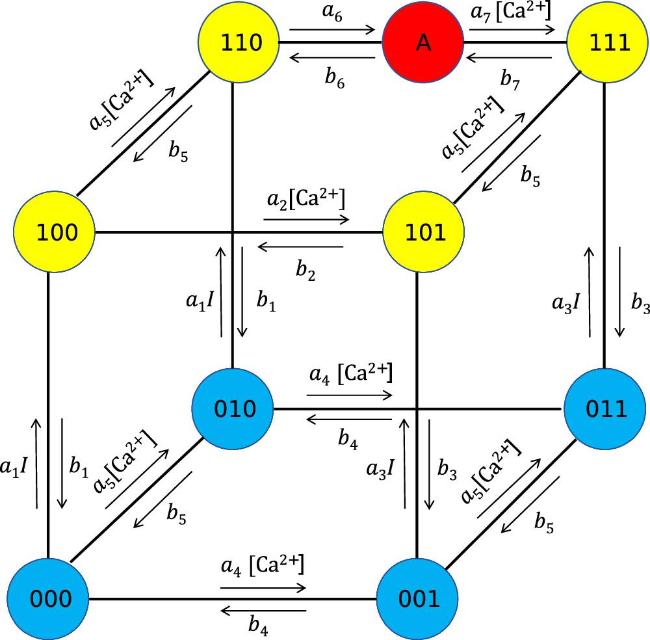
Figure 1. Nine-state model of the IP3R channel classified by binding status. Blue-filled circles represent states where IP3 is unbound, yellow-filled circles indicate states where IP3 is bound, and red-filled circles denote the fully activated state A. The 110 state is the pre-activated state. Arrows represent state transitions, with transition rates influenced by IP3 and Ca2+ concentrations. |
By incorporating structural insights from cryo-EM studies, our model offers a refined perspective on IP3R channel dynamics. Earlier models, such as the nine-state model by Shuai et al [22], distinguished between pre-activated and activated states but were developed without structural data. In these models, the activated state A was directly connected only to the pre-activated 110 state, with inhibition occurring at the 110 state. However, cryo-EM studies reveal that the pre-activated state is an obligatory intermediate before full activation and, importantly, that inhibition occurs only after activation, rather than at the pre-activated stage [27]. Consequently, in our model, the activated state is positioned between the pre-activated 110 state and the inhibited 111 state.
The transition rates between states depend on the concentrations of signaling molecules and their associated rate constants, as shown in figure 1. In this model, we assume that Ca2+ binding follows diffusion-limited kinetics, leading to a linear dependence on cytosolic [Ca2+]. This is justified by the fact that physiological Ca2+ concentrations (typically 0.001–10 μM) are well below the saturation levels of most binding sites, where binding is governed by diffusional encounter rates. Such linear dependence has also been widely adopted in classical models of IP3Rs, including the DYK model and its extensions [17, 22, 23]. The specific rate constants for these transitions are listed in table 1.
Table 1. Parameter values used in the nine-state model of IP3R. Parameters highlighted in bold are newly introduced in our model and are fitted based on data from [27]. All other parameters are adopted from the DYK model [17]. The symbol δr denotes the change in the Pearson correlation coefficient resulting from a 50% variation of the corresponding parameter. |
| Parameter | Value | Unit | δr | Description |
|---|---|---|---|---|
| a1 | 400 | μM−1s−1 | 0.006 | IP3 (binding) |
| a2 | 0.2 | μM−1s−1 | 0.002 | Ca2+ (binding) |
| a3 | 400 | μM−1s−1 | 0.030 | IP3 (binding) |
| a4 | 0.2 | μM−1s−1 | 0.001 | Ca2+ (binding) |
| a5 | 20 | μM−1s−1 | 0.094 | Ca2+ (binding) |
| a6 | 80 | s−1 | 0.111 | Ca2+ (activation) |
| a7 | 0.2 | μM−1s−1 | 0.089 | Ca2+ (inhibition) |
| b1 | 52 | s−1 | 0.004 | IP3 (unbinding) |
| b2 | 0.2098 | s−1 | 0.031 | Ca2+ (unbinding) |
| b3 | 377.36 | s−1 | 0.019 | IP3 (unbinding) |
| b4 | 0.0289 | s−1 | 0.006 | Ca2+ (unbinding) |
| b5 | 1.6468 | s−1 | 0.070 | Ca2+ (unbinding) |
| b6 | 100 | s−1 | 0.093 | Ca2+ (inactivation) |
| b7 | 0.2098 | s−1 | 0.040 | Ca2+ (activation) |
Most of the parameters in our model are adapted from the classical DYK model, which provides well-established rate constants for Ca2+ and IP3 binding and unbinding (parameter pairs a1–b1, a2–b2, ..., a5–b5) [17]. These parameters primarily determine the affinities of the activation and inhibition sites and have been widely used in previous IP3R modeling studies. For the newly introduced transition rates governing the pre-activated to conducting states (a6–b6 and a7–b7), no direct experimental measurements are available for these rates. We determine a6–b6 and a7–b7 by minimizing the discrepancy—quantified via the Pearson correlation coefficient r—between the model-predicted and experimentally observed state distributions across a range of fixed Ca2+ concentrations under saturated IP3 conditions, as revealed by cryo-EM [27]. This structure-based fitting ensures that the model captures gating dynamics consistent with observed conformational states. Moreover, the fitted parameters are further validated by demonstrating that the model reproduces physiologically relevant calcium oscillations, thereby linking structural data with functional calcium signaling behavior.
The resulting fit yields a Pearson correlation of r = 0.628 between simulated and experimental state distributions. To evaluate the sensitivity of the model, we examined how a 50% variation in each parameter affects the Pearson correlation coefficient r. For completeness, we also report the sensitivity results for the fixed parameters, to provide a broader context. The resulting change in correlation, denoted by δr, indicates that variations in a5, a6, a7, b5, and b6 each lead to a change in δr of approximately 0.1, suggesting these parameters have a substantial impact on model performance. In contrast, variations in the remaining parameters result in significantly smaller changes, with δr consistently below 0.05.
Early models, such as the DYK model, assumed that although IP3R is a tetramer, only three equivalent and independent subunits contribute to conduction. In this simplified framework, the channel was considered open only when all three subunits were in the activated state (which is also the 110 state, as the pre-activated and activated states were not differentiated in these models), leading to an open probability of ${P}_{{\rm{O}}}={x}^{3}$ with ${X}_{\mathrm{A}}$ being the probability of activated state A [17, 21]. However, in reality, the IP3R functions as a tetramer, with each monomer’s activation regulated by both IP3 and Ca2+. Recent experimental and theoretical studies tend to favor the idea that subunit interactions play a crucial role, and the channel opens only when at least three of the four subunits are in the activated state [22–24]. Therefore, the open probability is given by
$\begin{eqnarray}{P}_{{\rm{O}}}={P}_{{\rm{4O}}}+{P}_{{\rm{3O}}}={x}_{A}^{4}+4{x}_{A}^{3}(1-{x}_{A}).\end{eqnarray}$
In this work, we use a DYK-based mean-field model, which captures the averaged oscillatory behavior of IP3R channel populations. The model does not explicitly include spatial coordination among channels, so the simulated oscillations reflect collective dynamics rather than local events near individual channels.To simulate calcium oscillations, it is crucial to account for calcium exchange between the cytosol and the ER. In this study, we adopt the simplified framework of the DYK model, which has been widely used in formulating the differential equations governing calcium dynamics in both compartments [17, 18, 32, 33]. The calcium concentration in the cytoplasm evolves according to the differential equation
$\begin{eqnarray}\frac{{\rm{d}}[{\,\rm{Ca}\,}^{2+}]}{{\rm{d}}t}={J}_{\rm{in}\,}-{J}_{\,\rm{out}},\end{eqnarray}$
where [Ca2+] represents the free Ca2+ concentration in the cytoplasm. Calcium influx primarily occurs through two mechanisms: IP3R-mediated release and passive leakage, which together contribute to $\begin{eqnarray}{J}_{\,\rm{in}\,}={c}_{1}({\nu }_{1}{P}_{{\rm{O}}}+{\nu }_{2})\left({[{\,\rm{Ca}\,}^{2+}]}_{\,\rm{ER}\,}-[{\,\rm{Ca}\,}^{2+}]\right).\end{eqnarray}$
Here, ${[{\,\rm{Ca}\,}^{2+}]}_{\,\rm{ER}\,}$ is the Ca2+ concentration in the ER, and c1 denotes the volume ratio between the ER and the cytoplasm. The first term, ν1PO, represents Ca2+ release through the IP3R channel, where ν1 is the maximum flux and PO denotes the channel open probability. The second term, ν2, accounts for passive Ca2+ leakage through non-gated channels. To ensure conservation of total Ca2+ within the system, we impose the constraint ${c}_{0}={[{\,\rm{Ca}\,}^{2+}]}_{\,\rm{ER}\,}+[{\,\rm{Ca}\,}^{2+}]$.In our model, we assume that the maximum flux is identical for states with either three or four activated subunits. Currently, there is no direct experimental evidence linking the number of activated subunits to distinct unitary flux levels. Although single-channel recordings have revealed multiple conductance states, the precise relationship between these states and subunit activation remains unclear [34]. Alzayady et al demonstrated that full channel activation under physiological conditions requires all four subunits to be activated [35], whereas the classical DYK model assumes that three activated subunits suffice for channel opening. Nonetheless, several modeling studies allow both 3/4- and 4/4-activated states to be conductive, often assuming comparable maximal flux [22, 36]. We adopt this modeling convention as it simplifies the analysis and avoids introducing parameters currently unconstrained by experimental data.
The primary mechanism for transporting Ca2+ from the cytoplasm back into the ER is the Sarcoplasmic Endoplasmic Reticulum Ca2+-ATPase (SERCA) calcium pump. This calcium efflux is governed by a second-order Hill equation,
$\begin{eqnarray}{J}_{\,\rm{out}\,}=\frac{{\nu }_{3}{[{\,\rm{Ca}\,}^{2+}]}^{2}}{{[{\,\rm{Ca}\,}^{2+}]}^{2}+{k}_{3}^{2}},\end{eqnarray}$
where ν3 represents the maximum calcium uptake rate of the SERCA pump, and k3 is the activation constant. The key parameters used in these equations are summarized in table 2.Table 2. Parameters for the exchange of calcium between the cytosol and the ER [17]. |
| Parameter | Value | Description |
|---|---|---|
| c0 | 2.0 μM | Total [Ca2+] in terms of cytosolic volume |
| c1 | 0.185 | (ER volume)/(cytosolic volume) |
| ν1 | 6 s−1 | Max Ca2+ channel flux |
| ν2 | 0.11 s−1 | Ca2+ leak flux constant |
| ν3 | 0.9 μM−1s−1 | Max Ca2+ uptake |
| k3 | 0.1 μM | Activation constant for ATP-Ca2+ pump |
3. Results
3.1. Methodology
We developed an IP3R state transition model that incorporates calcium exchange between the cytosol and the ER. This model aims to reproduce the state distribution of the human IP3R reported by Paknejad et al [27]. By coupling the IP3R model with calcium cycling dynamics, we simulate IP3R-dependent Ca2+ oscillations and explore the functional roles of different IP3R states.
To obtain the equilibrium state distributions under varying calcium ion concentrations ([Ca2+]), we employed a nine-state transition rate matrix framework. We defined a state probability vector P(t) and constructed a 9 × 9 transition rate matrix K, which captures all possible transitions between states. Off-diagonal elements K(j, i) represent transition rates from state i to state j, while diagonal elements K(i, i) correspond to the total rate of leaving state i. These transitions mainly reflect IP3 and Ca2+ binding/unbinding events, making transition rates dependent on ligand concentrations as well as ligand-independent conformational changes.
The steady-state distribution was obtained by numerically solving K · P = 0 with normalization of P. This calculation was performed using Julia’s Differentialequations.jl package, leveraging its robust solvers for linear systems. We computed the state distributions over a physiologically relevant range of calcium concentrations (100 to 10000 nM), enabling a detailed representation of how Ca2+ modulates IP3R state probabilities. Incorporating the flux expression from equation (2 ), we then simulate calcium oscillation dynamics by solving the resulting nonlinear system.
3.2. Distribution of IP3R states under saturated IP3 conditions
EM studies were conducted under conditions of saturated IP3, with several fixed Ca2+ concentration levels [27]. To mirror these experimental conditions, we perform simulations with 2 μM IP3, while maintaining Ca2+ concentrations at 1, 10, 102, 103, and 104 nM, following the experimental methodology in [27]. Since the Ca2+ concentration remained constant, calcium exchange between the cytosol and the ER is not considered. The state distribution is determined solely based on the nine-state IP3R model. Given that IP3 is saturated, only states where IP3 is bound are relevant. We compare the distributions of four key states (100, 110, A, and 111) with experimental EM data, as shown in figure 2.
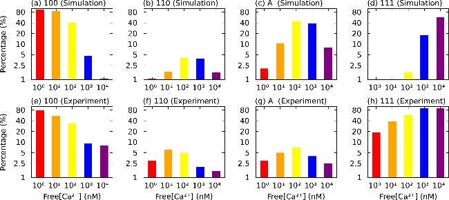
Figure 2. State distribution at different fixed Ca2+ concentrations under saturated IP3 condition. The patterns in a, b, c, and d depict the simulated state distributions of the 100, 110, A, and 111 states at varying orders of magnitude of Ca2+ concentration, respectively. The patterns in e, f, g, and h show the corresponding state distributions reported from the results of EM experiments [27]. Both the simulations and experiments were conducted with IP3 = 2 μM. |
To quantitatively assess the agreement between our simulated and experimentally observed state distributions, we compute the Pearson correlation coefficient between the predicted and measured state distributions. The resulting correlation coefficient is r = 0.628, which indicates a moderate-to-strong agreement. While this level of correlation is not perfect, it reflects that the model captures the key trends in the relative state occupancies.
It is important to note that the experimental state distributions derived from cryo-EM data are inherently subject to multiple sources of uncertainty, including classification noise during 3D reconstruction, limited particle numbers, and biological heterogeneity across IP3R tetramers. Furthermore, variations in calcium buffering and sample preparation may also influence the measured conformational occupancies. Considering these factors, a correlation of this magnitude supports the reliability of our model in capturing the essential behavior of the IP3R gating landscape.
Our results reveal a distinct Ca2+-dependent distribution of IP3R states. At low Ca2+ concentrations (<10 nM), the majority of IP3Rs reside in the 100 state, where the receptor is bound to IP3 but remains unbound to Ca2+. As Ca2+ concentration increases, IP3Rs gradually transition to the pre-activated 110 state, where one Ca2+ ion is bound. This pre-activated state serves as an intermediate, facilitating subsequent activation into the A state. The relative abundance of the activated A state reaches its peak (43.4%) when [Ca2+] is within 102 nM. However, at very high Ca2+ concentrations (>104 nM), the receptor undergoes inhibition, with most molecules transitioning into the 111 state, in which both Ca2+-binding sites are occupied. These trends in the four states presented here closely align with electron microscopy data, as shown in the lower four patterns of figure 2 [27].
The distributions of individual receptor states exhibit characteristic trends across the full range of Ca2+ concentrations. As expected, the occupancy of the 100 state decreases with increasing [Ca2+], while the 111 state increases. In contrast, both the pre-activated 110 and activated A states follow a biphasic pattern: their relative abundances initially increase with [Ca2+], reaching a peak before declining at higher concentrations. This bell-shaped distribution is consistent with previous electrophysiological recordings and theoretical studies [17, 18, 37, 38], confirming that IP3Rs exhibit a well-defined biphasic activation profile.
3.3. Open probability at different IP3R concentrations and role of IP3 state
To assess the functional significance of different states in our model, we systematically removed the 001, 101, and 010 states from the original nine-state IP3R channel model, generating three simplified versions. Using these models, we conducted numerical simulations to analyze the opening probability PO as a function of [Ca2+] concentration under varying IP3 levels, considering only IP3R state transitions.
The results, presented in figure 3, demonstrate that all models retain a bell-shaped PO curve, indicating that the fundamental dependence of IP3R activity on [Ca2+] remains intact despite the removal of specific states. This observation is consistent with the findings of Shuai et al [23], who reported that the 001 and 101 states could be omitted without significantly altering the channel’s functional behavior. Notably, the full nine-state model provides predictions that closely match experimental data [39, 40], underscoring its ability to accurately capture the Ca2+-dependent regulation of IP3Rs.
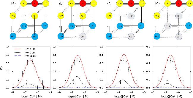
Figure 3. Comparison of the nine-state model and three simplified models obtained by sequentially removing the 001, 101, and 010 states (gray indicates removed states). The lower panel shows the simulated open probability (PO) for each model alongside experimental data from single-channel patch-clamp recordings of IP3R on the native nuclear membrane. Circles represent data for [IP3] = 0.2 μM, while stars indicate data for [IP3] = 0.01 μM [39, 40]. |
The overall bell-shaped dependence of PO on [Ca2+] remains largely unchanged across different models. At IP3 concentration [IP3] = 2.0 μM, the nine-state model predicts a peak PO of 0.35 at [Ca2+] = 10−6.6M. Minor variations are observed in peak PO when modifying the model, with the removal of the 001 state slightly increasing the maximum PO to 0.4. Additional adjustments involving the 101 and 010 states result in negligible further changes, suggesting that the fundamental channel behavior remains intact, with only minor contributions from these states at high IP3 concentrations.
At lower IP3 concentrations ([IP3] = 0.1 μM), the effect of the 001 state is slightly more noticeable, with the full nine-state model predicting a peak PO of 0.05. The absence of the 001 state shifts the peak of the PO curve toward a lower [Ca2+] concentration, indicating a mild influence on calcium sensitivity. However, the removal of the 101 and 010 states introduces little additional change, reaffirming that the overall regulatory dynamics are preserved across models.
At very low IP3 concentrations ([IP3] = 0.01 μM), all models predict an opening probability near zero, indicating that such low IP3 levels are insufficient to activate the channel. This result aligns with experimental observations [35], further confirming the model’s validity. Under these minimal IP3 conditions, differences between models become negligible, underscoring the dominant role of IP3 binding in regulating channel activity.
3.4. Calcium oscillation
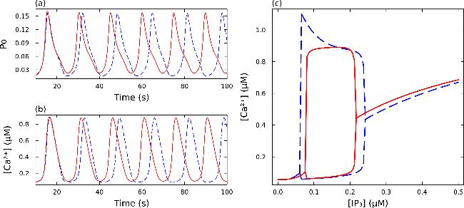
Using both the nine-state and simplified six-state models, we simulated calcium oscillations by incorporating the differential equations governing calcium concentration dynamics in the cytoplasm and ER, as described in equation (2 ). Under an IP3 concentration of 0.2 μM, the models successfully reproduced calcium oscillations. The results in figures 4(a) and (b) show that the oscillation period in the cytoplasm obtained with the nine-state model is approximately 14.8 s, matching experimentally observed oscillation periods in non-excitable cells [41, 42]. The maximum open probability, PO, reaches approximately 0.16. When using the six-state model, the oscillation period increases slightly, while both the oscillation amplitude and PO remain nearly unchanged. Further testing, by turning off additional states, confirmed that these states are essential for reproducing the oscillatory behavior.
Figure 4. Calcium oscillations. (a) Variation in open probability over time. (b) Variation in calcium concentration [Ca2+] over time. (c) Bifurcation diagram of calcium concentration as a function of [IP3] levels. In all panels, the red solid line represents the nine-state model and the blue dashed line represents the six-state model. |
To provide a more comprehensive picture of calcium oscillations in our model, we present bifurcation diagrams for [IP3] and [Ca2+] derived from both the nine-state and six-state models in figure 4(c). Unlike the DYK model, our model demonstrates increased sensitivity to [IP3], enabling oscillations to occur at lower IP3 concentrations. In the nine-state model, calcium oscillations first appear when the [IP3] concentration exceeds 0.08μM. These oscillations remain stable within the range of 0.1–0.2 μM, maintaining a relatively constant amplitude. However, as [IP3] increases further, the oscillation amplitude abruptly vanishes when [IP3] approaches 0.22 μM. Although the six-state model begins to exhibit oscillations at a slightly lower [IP3] threshold of 0.065 μM—where [Ca2+] peaks at 1.10 μM—its overall dynamic behavior remains highly consistent with that of the full nine-state model.
While both the original DYK model with eight states and our model display an [IP3] window for calcium oscillations, a key distinction lies in our model, which incorporates pre-activated states. In our model, the oscillation amplitude shows a sharp, abrupt increase upon surpassing the [IP3] threshold. This increase occurs immediately, reaching its maximum value and remaining nearly constant for a brief period before diminishing. In contrast, the DYK model exhibits a more gradual increase in oscillation amplitude, with the peak occurring only after an [IP3] concentration increase of approximately 0.2 μM [17]. These results suggest that a critical [IP3] threshold exists, beyond which calcium binding is significantly accelerated. This rapid binding leads to the swift opening of multiple IP3R channels and the initiation of calcium oscillations. This mechanism emphasizes IP3’s ability to regulate calcium oscillations with high precision, ensuring that the oscillations can be finely controlled and stabilized within the system.
4. Summary and discussion
In this work, we developed a novel nine-state IP3R channel model incorporating pre-activated states, aligning it with recent EM findings. We calculated the distribution of IP3R states under saturating IP3 conditions and found the results comparable to the EM observations. Incorporating calcium exchange between the cytosol and the ER enables the reproduction of calcium oscillations, and is very consistent with the experimental result.
Our model replicates key features of Ca2+-dependent IP3R activation and inhibition observed in previous biochemical and electrophysiological experiments [18]. It reproduces similar trends in free Ca2+ levels across four selected states under saturating IP3 conditions, notably capturing the bell-shaped dependence for both the pre-activated and activated states. Although our results are qualitatively consistent with EM data [27], quantitative discrepancies persist. Structural studies suggest that some receptor subunits may remain unbound due to incomplete ligand occupancy or conformational heterogeneity [43]. Future refinements, such as incorporating partial IP3 occupancy or cooperative interactions between subunits, could help resolve these differences.
We also discuss the role of the states in the model. By removing the 001, 101, and 010 states, we found that the bell-shaped relationship between open probability (PO) and calcium concentration remained consistent, with the nine-state model closely matching experimental data. Although the six-state reduced model requires slightly lower IP3 concentrations to trigger calcium oscillations, it maintains similar periods and amplitudes. Such results suggest that the 001, 101, and 010 states may play minor roles in calcium signaling, at least in the case considered in the current work.
In our model, a key characteristic is that the calcium oscillation sharply initiates as the IP3 concentration rises, remaining at a constant amplitude during its course. Once it reaches a certain level, the oscillation abruptly ceases. This indicates that IP3 exerts a switch-like regulatory mechanism over the calcium oscillation, where the system displays an all-or-none response: no oscillation below a threshold, sustained oscillation with fixed amplitude above it, and termination beyond a higher threshold. This mechanism is crucial for cells that rely on binary signaling to regulate downstream processes.
A key contributor to the switch-like behavior observed in our simulations is the presence of a pre-activated intermediate state in the IP3R gating scheme. Cryo-EM structures of IP3R1 have revealed partially shifted conformations—such as contraction of the ARM2 domain—that are consistent with a primed, non-conductive state preceding full channel opening [27]. In our model, elevated IP3 stabilizes this intermediate conformation, resulting in a substantial accumulation of subunits in this state prior to Ca2+-dependent activation.
Because this intermediate lies energetically closer to the open state than the fully closed conformation, it reduces the activation barrier and shortens the latency between Ca2+ binding and channel opening. As a result, a modest increase in cytosolic Ca2+ can rapidly trigger the transition of many receptors from the intermediate to the open state, producing the steep, threshold-like Ca2+ release characteristic of figure 4.
In physiological contexts requiring precise control over calcium dynamics—such as neuronal signaling, immune cell activation, and hormone secretion—this mechanism ensures a rapid and coordinated cellular response. The constant oscillation amplitude observed after crossing the threshold can be interpreted as a frequency-encoded signaling mechanism, where the information is transmitted via oscillation frequency rather than amplitude variation. This mode of encoding is well established in various calcium-dependent pathways, including transcriptional regulation and enzyme activation [44, 45]. The presence of a pre-activated intermediate state thus provides a structural and dynamic basis for reliable on–off switching, stable amplitude generation, and frequency modulation, offering both precision and flexibility in cellular calcium signaling.
In conclusion, our findings highlight the importance of the pre-activated state in shaping threshold-dependent behavior, suggesting that the state is a fundamental feature of IP3R dynamics, enabling precise control over calcium-mediated cellular functions. It is vital for calcium signaling, allowing cells to rapidly switch between non-oscillatory and oscillatory states. These dynamics are crucial for various calcium-dependent processes, such as transcription regulation and enzyme activation, highlighting the model’s potential in understanding frequency-encoded signaling in cellular functions.