


1. Introduction
It is widely known that equilibrium thermodynamics is a well-established field with three laws of thermodynamics as hallmarks. However, most natural systems are not in the equilibrium state. They can exchange energy and matter with the environment and have finite driving forces [1]. To deal with them, we need to extend the concept of equilibrium thermodynamics to non-equilibrium. It is a great pity that the current field of non-equilibrium (or irreversible) thermodynamics has been divided into many different 'schools', including classical irreversible thermodynamics [2], rational thermodynamics [3], extended irreversible thermodynamics [4], the general equation for the non-equilibrium reversible-irreversible coupling (GENERIC) [5] and many others. Each school has its own starting point, assumptions, and ways of formulation, but all keep the same aim in mind——to construct thermodynamically compatible and mathematically rigorous models for new physical systems under non-equilibrium situations.
The failure of previous studies in constructing a unified general framework for non-equilibrium thermodynamics stems from the following challenges:
●Non-equilibrium phenomena, like bistability, memory-effect, and pattern formation, are far more complicated than those under the equilibrium state;
●Non-equilibrium systems are time-evolving and do not meet the requirement of time reversibility, meaning modeling by dynamical equations are more suitable (or easier) than a thermodynamic formulation;
●Many non-equilibrium phenomena are system-size dependent and cannot be dealt with from a macroscopic thermodynamic view;
●A microscopic theory for non-equilibrium systems, in analogy to Boltzmann's statistical mechanics for equilibrium systems, is still lacking.
Motivated by the gradient-conservative structure proposed by Mielke et al [6], in this study we propose that many different thermodynamic modeling approaches, including GENERIC [5], Onsager's variational principle [7], the energetic variational approach [8], and classical irreversible thermodynamics [4], can all be cast into the gradient-conservative structure, which therefore suggests a unified theoretical framework to model various non-equilibrium thermodynamic processes.
To be exact, in section 2 we first revisit the basic formulation of the gradient-conservative structure, its nice mathematical properties, close relations to the large deviations principle, and interpretation in Wasserstein space. Our main result, the unification of various thermodynamically compatible modeling approaches used in the field of non-equilibrium thermodynamics in the sense of the gradient-conservative structure, is demonstrated in section 3 . Section 4 includes two concrete examples, through which the consistency of different modeling approaches will be fully appreciated. The last section contains a brief conclusion and some preliminary discussion.
2. Gradient-conservative structure
2.1. Basic formulation
We introduce vector z = z(t) as a group of state variables on a Riemann manifold ${ \mathcal Z }$, whose time evolution is assumed to obey the following gradient-conservative structure (GCS) [9],
$\begin{eqnarray}\frac{{\rm{d}}{\boldsymbol{z}}}{{\rm{d}}t}={{\rm{\nabla }}}_{{\boldsymbol{\xi }}}{\psi }^{* }({\boldsymbol{z}},{\boldsymbol{\xi }}){| }_{{\boldsymbol{\xi }}=-{\rm{\nabla }}F({\boldsymbol{z}})}+{\boldsymbol{A}}({\boldsymbol{z}})\cdot {\rm{\nabla }}E({\boldsymbol{z}}).\end{eqnarray}$
Here, the first term on the right-hand side $\text { ∇ }$ξψ*(z, ξ)|ξ=-$\text { ∇ }$F(z) denotes the gradient dynamics with a non-negative dissipation function ψ*(z, ξ), whose minimum is attained at ξ = 0 (ψ*(z, 0) = 0), while the second term A(z) · $\text { ∇ }$E(z) presents the conservative dynamics. ${{\boldsymbol{A}}}^{{\mathbb{T}}}=-{\boldsymbol{A}}$ is an antisymmetric operator. E(z) is the total energy of the system, F(z) is the relative entropy or free energy function, where $\text { ∇ }$E and $\text { ∇ }$F denote the gradients of energy and free energy with respect to state variables z, respectively.Along with the gradient-conservative structure, two transverse conditions are further required, i.e.5 ) holds due to the Legendre-Fenchel transform, and the last inequality holds due to the non-negativity of ψ* and ψ, which will be further clarified below equation (7 ).
$\begin{eqnarray}{\left.{\rm{\nabla }}E({\boldsymbol{z}})\cdot \frac{\partial {\psi }^{* }({\boldsymbol{z}},{\boldsymbol{\xi }})}{\partial {\boldsymbol{\xi }}}\right|}_{{\boldsymbol{\xi }}=-{\rm{\nabla }}F}=0,\end{eqnarray}$
$\begin{eqnarray}{\rm{\nabla }}F({\boldsymbol{z}})\cdot {\boldsymbol{A}}({\boldsymbol{z}})\cdot {\rm{\nabla }}E({\boldsymbol{z}})=0.\end{eqnarray}$
As we will see, these two conditions guarantee that the system dynamics is compatible with the general laws of thermodynamics, that is, the energy conservation and relative entropy decreasing in time. $\begin{eqnarray}\frac{{\rm{d}}E({\boldsymbol{z}})}{{\rm{d}}t}={\rm{\nabla }}E({\boldsymbol{z}})\cdot \frac{{\rm{d}}{\boldsymbol{z}}}{{\rm{d}}t}={\rm{\nabla }}E({\boldsymbol{z}})\cdot {\boldsymbol{A}}({\boldsymbol{z}})\cdot {\rm{\nabla }}E({\boldsymbol{z}})=0,\end{eqnarray}$
$\begin{eqnarray}\begin{array}{rcl}\frac{{\rm{d}}F({\boldsymbol{z}})}{{\rm{d}}t} & = & {\left.{\rm{\nabla }}F({\boldsymbol{z}})\cdot \frac{\partial {\psi }^{* }({\boldsymbol{z}},{\boldsymbol{\xi }})}{\partial {\boldsymbol{\xi }}}\right|}_{{\boldsymbol{\xi }}=-{\rm{\nabla }}F}\\ & = & -[{\psi }^{* }({\boldsymbol{z}},-{\rm{\nabla }}F)+\psi ({\boldsymbol{z}},\dot{\tilde{{\boldsymbol{z}}}})]\leqslant 0,\end{array}\end{eqnarray}$
where $\dot{\tilde{{\boldsymbol{z}}}}=\frac{\partial {\psi }^{* }({\boldsymbol{z}},{\boldsymbol{\xi }})}{\partial {\boldsymbol{\xi }}}{| }_{{\boldsymbol{\xi }}=-{\rm{\nabla }}F}$ denotes the part of the gradient dynamics, and $\psi ({\boldsymbol{z}},\dot{\tilde{{\boldsymbol{z}}}})$ is the Legendre-Fenchel transform of ψ*(z, - $\text { ∇ }$F). The second equality in equation (It is important to note that the GCS, by construction, describes systems whose dynamics are thermodynamically compatible. The transverse conditions (2) and (3) are necessary and sufficient to enforce energy conservation and relative entropy decrease. The GCS finds applications in various systems, including the chemical reactions and diffusion equations discussed in section 4. Although GCS provides a general framework, it imposes specific structural constraints related to thermodynamic compatibility that not all dynamical systems satisfy. To illustrate this fact, we present a detailed counter-example.
Consider a damped harmonic oscillator described by dq/dt = p and dp/dt = -q - $\gamma$p, where ${\boldsymbol{z}}={(q,p)}^{{\mathbb{T}}}$ represents the phase space coordinates and $\gamma$ > 0 is the damping coefficient. If we attempt to represent this system within the GCS framework using the natural energy function $E=\frac{1}{2}({p}^{2}+{q}^{2})$ and the standard antisymmetric matrix ${\boldsymbol{A}}=\left[\begin{array}{cc}0 & 1\\ -1 & 0\end{array}\right]$, the dissipative component must satisfy ${\left({{\rm{\nabla }}}_{{\boldsymbol{\xi }}}{\psi }^{* }({\boldsymbol{z}},{\boldsymbol{\xi }})\right)}_{{\boldsymbol{\xi }}=-{\rm{\nabla }}F({\boldsymbol{z}})}$= dz/dt - A(z) · $\text { ∇ }$E(z) = ${(0,-\gamma p)}^{{\mathbb{T}}}$. This representation violates the transverse condition ${\rm{\nabla }}E({\boldsymbol{z}})\cdot {\left({{\rm{\nabla }}}_{{\boldsymbol{\xi }}}{\psi }^{* }({\boldsymbol{z}},{\boldsymbol{\xi }})\right)}_{{\boldsymbol{\xi }}=-{\rm{\nabla }}F({\boldsymbol{z}})}=0$, since the dot product yields -$\gamma$p2 ≠ 0 for non-zero p. Alternatively, if we set A = 0, the system would need to be a pure gradient flow. However, the vector field ${(p,-q-\gamma p)}^{{\mathbb{T}}}$ is not conservative (its curl is non-zero), precluding this representation. Thus, the damped harmonic oscillator cannot be simply cast into the standard GCS framework, as illustrated by the two methods proposed above.
Overall, the conservative part in the GCS defines a dynamics that conserves energy as equation (4 ). If the antisymmetric operator A(z) further satisfies the Jacobi identity, this part defines a Hamiltonian structure, which is familiar to physicists and mathematicians and will not be discussed further here. In contrast, there have been numerous significant mathematical advances concerning the dissipative part given through a gradient structure in recent years, which therefore is worthy of further discussion. To be specific, we will show how to extend the gradient structure into a much generalized system, and its intrinsic relation with stochastic processes through the large deviations principle, as well as an elegant interpretation in Wasserstein space instead of the classical Euclidean space.
2.2. Generalized gradient systems
The gradient structure in equation (1 ) can be introduced in a much broader way. The triple (z, ψ*, F) is called a generalized gradient system [6, 10], if it satisfies
$\begin{eqnarray}\psi ({\boldsymbol{z}},\dot{{\boldsymbol{z}}})+{\psi }^{* }({\boldsymbol{z}},-{\rm{\nabla }}F)+\langle {\rm{\nabla }}F,\dot{{\boldsymbol{z}}}\rangle =0,\end{eqnarray}$
where the relative entropy $F:{ \mathcal Z }\to {\mathbb{R}}$ for $\forall {\boldsymbol{z}}\in { \mathcal Z }$, ‹ · , · › represents the inner product. We denote the tangent and cotangent spaces of the Riemann manifold ${ \mathcal Z }$ as $T{ \mathcal Z }$ and ${T}^{* }{ \mathcal Z }$ separately. ψ* and ψ constitute a Legendre-Fenchel duality pair, $\begin{eqnarray}\left\{\begin{array}{l}\psi ({\boldsymbol{z}},{\boldsymbol{\zeta }})=\mathop{\sup }\limits_{{\boldsymbol{\xi }}\in {T}_{{\boldsymbol{z}}}^{* }{ \mathcal Z }}(\langle {\boldsymbol{\xi }},{\boldsymbol{\zeta }}\rangle -{\psi }^{* }({\boldsymbol{z}},{\boldsymbol{\xi }})),\\ {\psi }^{* }({\boldsymbol{z}},{\boldsymbol{\xi }})=\mathop{\sup }\limits_{{\boldsymbol{\zeta }}\in {T}_{{\boldsymbol{z}}}{ \mathcal Z }}(\langle {\boldsymbol{\xi }},{\boldsymbol{\zeta }}\rangle -\psi ({\boldsymbol{z}},{\boldsymbol{\zeta }})).\end{array}\right.\end{eqnarray}$
If ψ* is strictly convex and differentiable in ξ, the supremum in the first equation of (7 ) is attained at a unique $\bar{{\boldsymbol{\xi }}}\in {T}_{{\boldsymbol{z}}}^{* }{ \mathcal Z }$ satisfying the stationary condition ${\boldsymbol{\zeta }}={\left(\frac{\partial {\psi }^{* }({\boldsymbol{z}},{\boldsymbol{\xi }})}{\partial {\boldsymbol{\xi }}}\right)}_{{\boldsymbol{\xi }}=\bar{{\boldsymbol{\xi }}}({\boldsymbol{z}},{\boldsymbol{\zeta }})}$, which implies the identity: 7 ) too. According to the Fenchel-Young inequality, we always have 6 ) actually implies an equivalent form
$\begin{eqnarray*}\psi ({\boldsymbol{z}},{\boldsymbol{\zeta }})=\langle \bar{{\boldsymbol{\xi }}}({\boldsymbol{z}},{\boldsymbol{\zeta }}),{\boldsymbol{\zeta }}\rangle -{\psi }^{* }\left({\boldsymbol{z}},\bar{{\boldsymbol{\xi }}}({\boldsymbol{z}},{\boldsymbol{\zeta }})\right).\end{eqnarray*}$
As defined via a Legendre-Fenchel transform, ψ is guaranteed to be a convex function of $\zeta$. A similar conclusion holds for the second equation of ( $\begin{eqnarray}\psi ({\boldsymbol{z}},\dot{{\boldsymbol{z}}})+{\psi }^{* }({\boldsymbol{z}},-{\rm{\nabla }}F)+\langle {\rm{\nabla }}F,\dot{{\boldsymbol{z}}}\rangle \geqslant 0,\end{eqnarray}$
meaning that equation ( $\begin{eqnarray}\left\{\begin{array}{l}\dot{{\boldsymbol{z}}}(t)=\frac{\partial {\psi }^{* }({\boldsymbol{z}},{\boldsymbol{\xi }})}{\partial {\boldsymbol{\xi }}}{| }_{{\boldsymbol{\xi }}=-{\rm{\nabla }}F},\\ {\rm{\nabla }}F({\boldsymbol{z}})=-\frac{\partial \psi ({\boldsymbol{z}},{\boldsymbol{\zeta }})}{\partial {\boldsymbol{\zeta }}}{| }_{{\boldsymbol{\zeta }}=\dot{{\boldsymbol{z}}}}.\end{array}\right.\end{eqnarray}$
It is recognized that the first equation gives the dissipative part in the GCS.A generalized gradient system further requires that
1. ψ*(z, ξ) is convex with respect to the second argument ξ;
2. ψ*(z, ξ) ≥ 0 for $\forall {\boldsymbol{\xi }}\in {T}_{{\boldsymbol{z}}}^{* }{ \mathcal Z }$, and ψ*(z, 0) = 0;
3. ψ*(z, ξ) = ψ*(z, - ξ) for $\forall {\boldsymbol{z}}\in { \mathcal Z },\forall {\boldsymbol{\xi }}\in {T}_{{\boldsymbol{z}}}^{* }{ \mathcal Z }$.
The second requirement on ψ* will apply a dual requirement on ψ, since
$\begin{eqnarray*}\left\{\begin{array}{l}{\psi }^{* }({\boldsymbol{z}},{\bf{0}})=0\iff \psi ({\boldsymbol{z}},{\boldsymbol{\zeta }})\geqslant 0,\quad \forall {\boldsymbol{\zeta }}\in {T}_{{\boldsymbol{z}}}{ \mathcal Z },\\ \psi ({\boldsymbol{z}},{\bf{0}})=0\iff {\psi }^{* }({\boldsymbol{z}},{\boldsymbol{\xi }})\geqslant 0,\quad \forall {\boldsymbol{\xi }}\in {T}_{{\boldsymbol{z}}}^{* }{ \mathcal Z }.\end{array}\right.\end{eqnarray*}$
Now it is direct to show that $\begin{eqnarray*}\frac{{\rm{d}}F({\boldsymbol{z}})}{{\rm{d}}t}=\langle {\rm{\nabla }}F,\dot{{\boldsymbol{z}}}\rangle =-[\psi ({\boldsymbol{z}},\dot{{\boldsymbol{z}}})+{\psi }^{* }({\boldsymbol{z}},-{\rm{\nabla }}F)]\leqslant 0,\end{eqnarray*}$
a special case of general results on the GCS. The last requirement is equivalent to the time symmetry requirement on ψ, that is, $\psi(z, \zeta)=\psi(z,-\zeta)$ for all ${\boldsymbol{\zeta }}\in {T}_{{\boldsymbol{z}}}{ \mathcal Z }$. It is natural in many systems, in which velocities with opposite directions lead to the same dissipation.2.3. Relation to the large deviations principle
The generalized gradient system (6 ) has a close connection with the underlying stochastic processes, which is clarified through the principle of large deviations. Consider the following dynamics
$\begin{eqnarray}\left\{\begin{array}{l}\frac{{\rm{d}}}{{\rm{d}}t}{\boldsymbol{z}}(t)={\boldsymbol{R}}({\boldsymbol{z}}),\\ {\boldsymbol{z}}(0)={{\boldsymbol{z}}}_{0},\end{array}\right.\end{eqnarray}$
whose solution is given by {z(t)}0≤t≤T. Further, suppose the above dynamics is invariant under the time-reversal transformation.Let us make small random perturbations of {z(t)}0≤t≤T and consider the corresponding stochastic process ${\{{{\boldsymbol{z}}}_{\epsilon }(t)\}}_{0\leqslant t\leqslant T}$, where 0 < ε « 1 denotes the noise level. Following the philosophy of the Fredlin-Wentzell theory [11], we assume that the large deviations principle holds for ${\{{{\boldsymbol{z}}}_{\epsilon }(t)\}}_{0\leqslant t\leqslant T}$ under the condition of fixed zε(0) = z0 and zε(T) = zT and as ε → 0
$\begin{eqnarray}{\mathbb{P}}({\{{{\boldsymbol{z}}}_{\epsilon }(t)\}}_{0\leqslant t\leqslant T}={\{{\boldsymbol{z}}(t)\}}_{0\leqslant t\leqslant T})\asymp \exp \left[-\frac{1}{\epsilon }{\int }_{0}^{T}L({\boldsymbol{z}},\dot{{\boldsymbol{z}}}){\rm{d}}t\right],\end{eqnarray}$
in which the time integral of the Lagrangian gives the large deviations rate function (or action in physics). Notice that, in the limit of ε → 0, the stochastic differential equation (SDE) $\begin{eqnarray*}{\rm{d}}{{\boldsymbol{z}}}_{t}={\boldsymbol{R}}({{\boldsymbol{z}}}_{t})\,{\rm{d}}t+\sqrt{2\epsilon }\,{\rm{d}}{{\boldsymbol{W}}}_{t},\end{eqnarray*}$
is not the 'straightforward' first-order ordinary differential equation (ODE) dz/dt = R(z) but instead a second-order ODE from the Euler-Lagrange equation associated with $L({\boldsymbol{z}},\dot{{\boldsymbol{z}}})$ with boundary conditions at z(0) and z(T).Furthermore, we assume that the Lagrangian is time reversible, meaning there exists a function U = U(z) such that [6, 12]
$\begin{eqnarray}L({\boldsymbol{z}},\dot{{\boldsymbol{z}}})-L({\boldsymbol{z}},-\dot{{\boldsymbol{z}}})=2\langle {\rm{\nabla }}U,\dot{{\boldsymbol{z}}}\rangle ,\end{eqnarray}$
$\forall {\boldsymbol{z}}\in { \mathcal Z },\forall \dot{{\boldsymbol{z}}}\in {T}_{{\boldsymbol{z}}}{ \mathcal Z }$. Now we are ready to introduce the dissipation function: $\begin{eqnarray}{\psi }^{* }({\boldsymbol{z}},{\boldsymbol{\xi }})=H({\boldsymbol{z}},{\rm{\nabla }}U+{\boldsymbol{\xi }})-H({\boldsymbol{z}},{\rm{\nabla }}U),\end{eqnarray}$
in which the Hamiltonian function is defined as the Legendre-Fenchel transformation of the Lagrangian function, $\begin{eqnarray}H({\boldsymbol{z}},{\boldsymbol{\xi }})=\mathop{\sup }\limits_{\dot{{\boldsymbol{z}}}\in {T}_{{\boldsymbol{z}}}{ \mathcal Z }}(\langle {\boldsymbol{\xi }},\dot{{\boldsymbol{z}}}\rangle -L({\boldsymbol{z}},\dot{{\boldsymbol{z}}})).\end{eqnarray}$
Most importantly, the dissipation function defined above satisfies1. ψ*(z, ξ) is convex with respect to the second argument ξ;
2. ψ*(z, ξ) ≥ 0 $\forall {\boldsymbol{\xi }}\in {T}_{{\boldsymbol{z}}}^{* }{ \mathcal Z }$, and ψ*(z, 0) = 0;
3. ψ*(z, ξ) = ψ*(z, - ξ) $\forall {\boldsymbol{\xi }}\in {T}_{{\boldsymbol{z}}}^{* }{ \mathcal Z }$,
by recalling the mathematical properties of the large deviations rate function as well as the Legendre-Fenchel transformation. See Appendix A for a proof.
Defining $\psi ({\boldsymbol{z}},\dot{{\boldsymbol{z}}})={\sup }_{{\boldsymbol{\xi }}\in {T}_{{\boldsymbol{z}}}^{* }{ \mathcal Z }}(\langle {\boldsymbol{\xi }},\dot{{\boldsymbol{z}}}\rangle -{\psi }^{* }({\boldsymbol{z}},{\boldsymbol{\xi }}))$, it is straightforward to verify that the Lagrangian function has an alternative insightful expression through the dissipation function, i.e.15 ) provides a natural measurement of the deviations of stochastic processes from the deterministic gradient flow.
$\begin{eqnarray}L({\boldsymbol{z}},\dot{{\boldsymbol{z}}})=\psi ({\boldsymbol{z}},\dot{{\boldsymbol{z}}})+{\psi }^{* }({\boldsymbol{z}},-{\rm{\nabla }}U)+\langle {\rm{\nabla }}U,\dot{{\boldsymbol{z}}}\rangle \geqslant 0,\end{eqnarray}$
which is non-negative due to the Fenchel-Young inequality. In particular, when $L({\boldsymbol{z}},\dot{{\boldsymbol{z}}})=0$, we have $\begin{eqnarray*}\begin{array}{r}\psi ({\boldsymbol{z}},\dot{{\boldsymbol{z}}})+{\psi }^{* }({\boldsymbol{z}},-{\rm{\nabla }}U)+\langle {\rm{\nabla }}U,\dot{{\boldsymbol{z}}}\rangle =0,\end{array}\end{eqnarray*}$
meaning (z, ψ*, U) defines a generalized gradient system. As the large deviations rate function equals zero, the stochastic process ${\{{{\boldsymbol{z}}}_{\epsilon }(t)\}}_{0\leqslant t\lt T}$ converges to the deterministic one with probability one. It can be rewritten into the form of gradient flows, i.e. $\begin{eqnarray*}\begin{array}{r}{\left.\dot{{\boldsymbol{z}}}(t)=\frac{\partial {\psi }^{* }({\boldsymbol{z}},{\boldsymbol{\xi }})}{\partial {\boldsymbol{\xi }}}\right|}_{{\boldsymbol{\xi }}=-{\rm{\nabla }}U}.\end{array}\end{eqnarray*}$
Therefore, the Lagrangian function $L({\boldsymbol{z}},\dot{{\boldsymbol{z}}})\geqslant 0$ in equation (2.4. Interpretation of gradient flows in Wasserstein space
The universality of gradient structures was fully appreciated through the milestone work of Otto [13], in which he, for the first time, pointed out that many non-gradient dynamics could be reformulated into a gradient one by making a change in the metric of the space. To see this point, we turn to an alternative interpretation of gradient flows in Wasserstein space.
Given two functions ${h}_{1},{h}_{2}:{\rm{\Omega }}\to {\mathbb{R}}$ with $\int$Ωh1dx = $\int$Ωh2dx = 0, one can define their Wasserstein scalar product at ρ as
$\begin{eqnarray*}{\langle {h}_{1},{h}_{2}\rangle }_{\rho }:= {\int }_{{\rm{\Omega }}}({\nabla }_{{\boldsymbol{x}}}{\psi }_{1}\cdot {\nabla }_{{\boldsymbol{x}}}{\psi }_{2})\rho {\rm{d}}{\boldsymbol{x}}{\boldsymbol{,}}\end{eqnarray*}$
where $\begin{eqnarray*}\left\{\begin{array}{l}{{\rm{\nabla }}}_{{\boldsymbol{x}}}\cdot (\rho {{\rm{\nabla }}}_{{\boldsymbol{x}}}{\psi }_{i})=-{h}_{i}\,\,\rm{in}\,\,{\rm{\Omega }}\\ \overrightarrow{{\boldsymbol{n}}}\cdot {{\rm{\nabla }}}_{{\boldsymbol{x}}}{\psi }_{i}=0\,\,\rm{on}\,\,\partial {\rm{\Omega }}.\end{array}\right.\end{eqnarray*}$
$\text { ∇ }$x denotes the normal gradient in Euclidean space, and $\overrightarrow{{\boldsymbol{n}}}$ denotes the boundary normal vector.Now we can define the gradient of a functional in Wasserstein space.
Given a functional $F:{{ \mathcal P }}_{2}({\rm{\Omega }})\to {\mathbb{R}}$, its gradient with respect to the Wasserstein scalar product at $\bar{\rho }\in {{ \mathcal P }}_{2}({\rm{\Omega }})$ is the unique function ${{\rm{\nabla }}}_{{W}_{2}}F(\bar{\rho })$ (if it exists) such that
$\begin{eqnarray*}{\left\langle {\left.{{\rm{\nabla }}}_{{W}_{2}}F(\bar{\rho }),\frac{\partial {\rho }_{\epsilon }}{\partial \epsilon }\right|}_{\epsilon =0}\right\rangle }_{\bar{\rho }}={\left.\frac{{\rm{d}}}{{\rm{d}}\epsilon }\right|}_{\epsilon =0}F({\rho }_{\epsilon }),\end{eqnarray*}$
for any smooth curve ${\rho }_{\epsilon }:(-{\epsilon }_{0},{\epsilon }_{0})\to { \mathcal P }({\rm{\Omega }})$ with ${\rho }_{0}=\bar{\rho }$.Now with respect to functional $F:{{ \mathcal P }}_{2}({\rm{\Omega }})\to {\mathbb{R}}$ and the probability measure $\bar{\rho }\in {{ \mathcal P }}_{2}({\rm{\Omega }})$, let us denote by $\delta F(\bar{\rho })/\delta \rho $ its first ${{ \mathcal L }}^{2}$-variation, which is the function in ${{ \mathcal L }}^{2}({\rm{\Omega }})$ such that
$\begin{eqnarray}{\left.\frac{{\rm{d}}}{{\rm{d}}\epsilon }\right|}_{\epsilon =0}F({\rho }_{\epsilon })={\left.{\int }_{{\rm{\Omega }}}\frac{\delta F(\bar{\rho })}{\delta \rho }({\boldsymbol{x}})\frac{\partial {\rho }_{\epsilon }({\boldsymbol{x}})}{\partial \epsilon }\right|}_{\epsilon =0}{\rm{d}}{\boldsymbol{x}}.\end{eqnarray}$
Therefore, by the definition of the Wasserstein scalar product, we can deduce that $\begin{eqnarray}{{\rm{\nabla }}}_{{W}_{2}}F(\bar{\rho })=-{{\rm{\nabla }}}_{{\boldsymbol{x}}}\cdot \left({{\rm{\nabla }}}_{{\boldsymbol{x}}}\left(\frac{\delta F(\bar{\rho })}{\delta \rho }\right)\bar{\rho }\right).\end{eqnarray}$
Now we are ready to introduce gradient flows in Wasserstein space.Given a functional $F:{{ \mathcal P }}_{2}({\rm{\Omega }})\to {\mathbb{R}}$, a curve of probability measure $\rho :[0,T)\to {{ \mathcal P }}_{2}({\rm{\Omega }})$ is a gradient flow of F with respect to W2 and with starting point ${\bar{\rho }}_{0}$ if
$\begin{eqnarray*}\left\{\begin{array}{l}\displaystyle \frac{\partial {\rho }_{t}}{\partial t}=-{\nabla }_{{W}_{2}}F({\rho }_{t}),\\ {\rho }_{0}={\bar{\rho }}_{0},\end{array}\right.\end{eqnarray*}$
Considering the above definition of gradient flows and concrete formulas for the Wasserstein gradient of F, we could rewrite plenty of classical examples in mathematical physics into gradient flows in Wasserstein space [14].
i) Given $F(\rho )=\int \rho \mathrm{ln}\rho {\rm{d}}{\boldsymbol{x}}$, the Wasserstein gradient flow leads to the heat equation $\frac{\partial \rho }{\partial t}=-{{\rm{\nabla }}}_{{W}_{2}}{ \mathcal F }[\rho ]={{\rm{\Delta }}}_{{\boldsymbol{x}}}\rho .$
ii) Given $F(\rho )=\int [\rho \mathrm{ln}\rho +\rho V({\boldsymbol{x}})]{\rm{d}}{\boldsymbol{x}}$, the gradient flow gives the Fokker-Planck equation $\frac{\partial \rho }{\partial t}={{\rm{\Delta }}}_{{\boldsymbol{x}}}\rho \,+{{\rm{\nabla }}}_{{\boldsymbol{x}}}\cdot (\rho {{\rm{\nabla }}}_{{\boldsymbol{x}}}V).$
iii) Given $F(\rho )=\frac{1}{m-1}\int {\rho }^{m}{\rm{d}}{\boldsymbol{x}}$ for m > 1, the gradient flow gives the porous medium equation $\frac{\partial \rho }{\partial t}={{\rm{\Delta }}}_{{\boldsymbol{x}}}({\rho }^{m}).$
iv) Given F(ρ) = $\int$[U(ρ) + ρV(x)]dx + $\frac{1}{2}\int \int W({\boldsymbol{x}}$ -y)ρ(x)ρ(y)dxdy, the gradient flow gives the diffusion-advection-aggregation model $\frac{\partial \rho }{\partial t}$ = ${{\rm{\nabla }}}_{{\boldsymbol{x}}}\cdot \left\{\rho \left[{{\rm{\nabla }}}_{{\boldsymbol{x}}}{U}^{{\prime} }(\rho )\right.\right.$ + $\text { ∇ }$xV(x) + $\left.\left.({{\rm{\nabla }}}_{{\boldsymbol{x}}}W)\ast \rho \right]\right\}$, where ${U}^{{\prime} }(\rho )=\frac{\delta U(\rho )}{\delta \rho }$, W * ρ = $\int$W(x - y)ρ(y)dy.
3. Unifying various thermodynamically compatible modeling approaches
3.1. GENERIC
The fundamental equation for the GENERIC looks quite similar to that of the GCS [17],
$\begin{eqnarray}\frac{{\rm{d}}{\boldsymbol{z}}}{{\rm{d}}t}={\boldsymbol{M}}({\boldsymbol{z}})\cdot {\rm{\nabla }}S({\boldsymbol{z}})+{\boldsymbol{A}}({\boldsymbol{z}})\cdot {\rm{\nabla }}E({\boldsymbol{z}}).\end{eqnarray}$
The two contributions to the time evolution of z generated by the entropy S and the total energy E above are the irreversible and reversible contributions to dynamics, respectively. The so-called Poisson operator A is antisymmetric, whereas the friction operator M is both symmetric and positive semi-definite. Furthermore, the entropy function S(z) is assumed to a convex function.Equation (18 ) is supplemented by two complementary degeneracy requirements, 18 ), independent of the particular form of the Hamiltonian.
$\begin{eqnarray}{\boldsymbol{M}}({\boldsymbol{z}})\cdot {\rm{\nabla }}E({\boldsymbol{z}})=0,\end{eqnarray}$
$\begin{eqnarray}{\boldsymbol{A}}({\boldsymbol{z}})\cdot {\rm{\nabla }}S({\boldsymbol{z}})=0.\end{eqnarray}$
The first requirement that the energy gradient $\text { ∇ }$E(z) is in the null-space of the friction operator M expresses the conservation of the total energy in a closed system by the irreversible contribution to the dynamics. On the other hand, the second requirement that the entropy gradient $\text { ∇ }$S(z) is in the null-space of the Poisson operator A expresses the reversible nature of the second term in equation (Under the help of degeneracy requirements, it becomes straightforward to show dE/dt = 0 and dS/dt ≥ 0, in accordance with the first and second laws of thermodynamics. Therefore, there is a nice one-to-one correspondence between the degeneracy requirements in the GENERIC and the transverse conditions in the GCS.
Provided that the dissipation function takes a quadratic form of ξ = - $\text { ∇ }$ F, i.e. ${\psi }^{* }({\boldsymbol{z}},{\boldsymbol{\xi }})=\frac{1}{2}\langle {\boldsymbol{\xi }},{\boldsymbol{M}}({\boldsymbol{z}}){\boldsymbol{\xi }}\rangle $, and replacing the relative entropy function F by its counterpart, the negative entropy function, -S, we see the GCS turns into the GENERIC mentioned above. Actually, the gradient structure has also been widely used to reformulate the GENERIC in recent years [9].
3.2. Onsager's variational principle
Onsager's variational principle (OVP) was originally proposed by Lars Onsager in 1931. In two seminal papers [18, 19], he not only established the famous reciprocal relation but also proposed the OVP as a variational principle which is equivalent to the linear force-flux relations in describing irreversible processes.
For isothermal systems, the OVP assumes the state variables follow the dynamic path that minimizes the so-called Rayleighian by Masao Doi [7], i.e.
$\begin{eqnarray}{ \mathcal R }({\boldsymbol{z}},\dot{{\boldsymbol{z}}})=\psi ({\boldsymbol{z}},\dot{{\boldsymbol{z}}})+\dot{F}({\boldsymbol{z}},\dot{{\boldsymbol{z}}}).\end{eqnarray}$
Here $\psi ({\boldsymbol{z}},\dot{{\boldsymbol{z}}})$ is the dissipation function, which is usually taken as a quadratic function of $\dot{{\boldsymbol{z}}}$, i.e. $\psi ({\boldsymbol{z}},\dot{{\boldsymbol{z}}})=\frac{1}{2}\langle \dot{{\boldsymbol{z}}},{\boldsymbol{M}}({\boldsymbol{z}})\dot{{\boldsymbol{z}}}\rangle $. M(z) is a positive definite operator and symmetric due to Onsager's reciprocal relations. $\dot{F}({\boldsymbol{z}},\dot{{\boldsymbol{z}}})=\langle {\rm{\nabla }}F({\boldsymbol{z}}),\dot{{\boldsymbol{z}}}\rangle $ represents the change rate of free energy. Then the Euler-Lagrange equation for minimizing ${ \mathcal R }$ with respect to $\dot{{\boldsymbol{z}}}$ is given by [20, 21] $\begin{eqnarray}{\boldsymbol{M}}({\boldsymbol{z}})\dot{{\boldsymbol{z}}}=-{\rm{\nabla }}F({\boldsymbol{z}}).\end{eqnarray}$
Therefore, the OVP can be regarded as an extension of the principle of the least dissipation of energy proposed by Lord Rayleigh [22].The statistical mechanical foundation of OVP was established by Onsager and Machlup in 1953 [23], which is known as the Onsager-Machlup variational principle [21]. The latter states that, with respect to the overdamped Langevin equation, the most probable transition path occurring between state z(t) and its nearby state $\tilde{{\boldsymbol{z}}}(t)$ is the one minimizing the Onsager-Machlup function or equivalently the Rayleighian function [24].
The relation between Onsager's variational principle and generalized gradient systems is straightforward. Consider the Lagrangian function 15 ), which is non-negative due to the Fenchel-Young inequality. Denote the sum of the first two terms as the Rayleighian
$\begin{eqnarray*}L({\boldsymbol{z}},\dot{{\boldsymbol{z}}})=\psi ({\boldsymbol{z}},\dot{{\boldsymbol{z}}})+\langle {\rm{\nabla }}F,\dot{{\boldsymbol{z}}}\rangle +{\psi }^{* }({\boldsymbol{z}},-{\rm{\nabla }}F)\geqslant 0,\end{eqnarray*}$
defined in equation ( $\begin{eqnarray}{ \mathcal R }({\boldsymbol{z}},\dot{{\boldsymbol{z}}})=\psi ({\boldsymbol{z}},\dot{{\boldsymbol{z}}})+\langle {\rm{\nabla }}F,\dot{{\boldsymbol{z}}}\rangle ,\end{eqnarray}$
in which the second term is exactly the change rate of free energy. It is apparent that the condition for generalized gradient flows ($L({\boldsymbol{z}},\dot{{\boldsymbol{z}}})=0$) implies Onsager's variational principle, $\begin{eqnarray}\frac{\partial L({\boldsymbol{z}},\dot{{\boldsymbol{z}}})}{\partial \dot{{\boldsymbol{z}}}}=\frac{\partial { \mathcal R }({\boldsymbol{z}},\dot{{\boldsymbol{z}}})}{\partial \dot{{\boldsymbol{z}}}}=0.\end{eqnarray}$
3.3. Energetic variational approach
The energetic variational approach (EVA) was proposed by Liu et al for modeling complex fluids systems in physics, chemistry, and biochemistry [8, 25-27]. The starting point of EVA is an energy-dissipation law 25 ), with ∆E = ∆S and E = K + F, where F = U - TS is the Helmholtz free energy.
$\begin{eqnarray}\frac{{\rm{d}}E}{{\rm{d}}t}=-{{\rm{\Delta }}}_{E}\leqslant 0,\end{eqnarray}$
where E denotes the total energy of the system, and ∆E represents the rate of energy dissipation. It can be obtained by a combination of the first and second laws of thermodynamics for an isothermal and mechanically isolated system, that is $\begin{eqnarray}\frac{{\rm{d}}}{{\rm{d}}t}(K+U)=\dot{W}+\dot{Q},\end{eqnarray}$
$\begin{eqnarray}T\frac{{\rm{d}}S}{{\rm{d}}t}=\dot{Q}+{{\rm{\Delta }}}_{S}.\end{eqnarray}$
Here K, U, S, and T represent the kinetic energy, internal energy, entropy, and absolute temperature. $\dot{W},\dot{Q},{{\rm{\Delta }}}_{S}$ denote the rates of the external work, heat absorption, and entropy production, separately. By subtracting the above two equations and using the isothermal and mechanically isolated conditions ${\rm{d}}T/{\rm{d}}t=\dot{W}=0$, we can derive the energy-dissipation law, equation (With respect to the energy-dissipation law in equation (25 ), the EVA assumes that the dynamics of a system is determined by a combination of the least action principle (LAP) and the maximum dissipation principle (MDP). The LAP, which states the conservative force of a Hamiltonian system, can be derived by taking the variation of the action functional ${A}_{F}={\int }_{0}^{t}(K-F){\rm{d}}\tau $ with respect to the state variable z. Meanwhile, the MDP shows that the dissipation force is given by a variation of the dissipation potential ψ with respect to the velocity $\dot{{\boldsymbol{z}}}$. In turn, the force balance condition leads to the underlying evolution equation of the system
$\begin{eqnarray}\frac{\partial {A}_{F}({\boldsymbol{z}},\dot{{\boldsymbol{z}}})}{\partial {\boldsymbol{z}}}=\frac{\partial \psi ({\boldsymbol{z}},\dot{{\boldsymbol{z}}})}{\partial \dot{{\boldsymbol{z}}}}.\end{eqnarray}$
The relation between EVA and the generalized gradient system can be understood through the following discussion. Consider the Lagrangian function 24 ) and (29 ) demonstrates the close connection between Onsager's variational approach and the EVA. Both of them take a quite similar form, except that the latter has an addition term, $-\frac{\partial K}{\partial {\boldsymbol{z}}}$.
$\begin{eqnarray*}\begin{array}{r}L({\boldsymbol{z}},\dot{{\boldsymbol{z}}})=\psi ({\boldsymbol{z}},\dot{{\boldsymbol{z}}})+\langle {\boldsymbol{\xi }},\dot{{\boldsymbol{z}}}\rangle +{\psi }^{* }({\boldsymbol{z}},-{\boldsymbol{\xi }}),\end{array}\end{eqnarray*}$
whose minimization gives $\begin{eqnarray}\frac{\partial L({\boldsymbol{z}},\dot{{\boldsymbol{z}}})}{\partial \dot{{\boldsymbol{z}}}}=\frac{\partial \psi ({\boldsymbol{z}},\dot{{\boldsymbol{z}}})}{\partial \dot{{\boldsymbol{z}}}}+{\boldsymbol{\xi }}={\bf{0}}.\end{eqnarray}$
Provided the conservative force ${\boldsymbol{\xi }}=-\frac{\partial {A}_{F}}{\partial {\boldsymbol{z}}}$, we arrive at the central equation of the EVA. A further comparison between equations (3.4. Classical irreversible thermodynamics and beyond
Classical irreversible thermodynamics (CIT) also started with the pioneering works of Onsager [18, 19] and later was formulated into a general framework for modeling various irreversible processes by Glansdorff, Prigogine, de Groot, Mazur, and many others [2]. The theoretical foundation of CIT lays on two key assumptions: (a) the local equilibrium hypothesis, which secures a spatiotemporal entropy density function; (b) a linear thermodynamic force-flux relationship.
To derive thermodynamically compatible equations for the time evolution of state variables z(t), CIT assumes the existence of a convex entropy function S(t) = S(z(t)) with respect to z(t). Then the famous Gibbs relation gives
$\begin{eqnarray}\frac{{\rm{d}}S}{{\rm{d}}t}=\frac{1}{T}\left(\frac{{\rm{d}}U}{{\rm{d}}t}-\frac{{\rm{d}}F}{{\rm{d}}t}\right)=\frac{1}{T}\left(\frac{\partial U}{\partial {\boldsymbol{z}}}\frac{{\rm{d}}{\boldsymbol{z}}}{{\rm{d}}t}-\frac{\partial F}{\partial {\boldsymbol{z}}}\frac{{\rm{d}}{\boldsymbol{z}}}{{\rm{d}}t}\right),\end{eqnarray}$
where U and F denote the internal energy and free energy, respectively. T stands for the temperature, which is a constant.Using the decomposition
$\begin{eqnarray*}\frac{{\rm{d}}{\boldsymbol{z}}}{{\rm{d}}t}={}G({\boldsymbol{z}})+{}C({\boldsymbol{z}}),\end{eqnarray*}$
where G(z) and C(z) represent the gradient dynamics and conservative dynamics respectively, we have $\begin{eqnarray}\begin{array}{rcl}\frac{{\rm{d}}S}{{\rm{d}}t} & = & \frac{1}{T}\left(\frac{\partial U}{\partial {\boldsymbol{z}}}{}G({\boldsymbol{z}})+\frac{\partial U}{\partial {\boldsymbol{z}}}{}C({\boldsymbol{z}})-\frac{\partial F}{\partial {\boldsymbol{z}}}{}C({\boldsymbol{z}})\right)-\frac{1}{T}\frac{\partial F}{\partial {\boldsymbol{z}}}{}G({\boldsymbol{z}}),\\ & = & {J}_{f}+{\rm{e}}{\rm{p}}{\rm{r}},\end{array}\end{eqnarray}$
where Jf and epr represent the entropy exchange rate and entropy production rate separately.Inspired by the formulation of the GENERIC, we set
$\begin{eqnarray}{ \mathcal G }({\boldsymbol{z}})=-{\boldsymbol{M}}({\boldsymbol{z}})\cdot \frac{\partial F}{\partial {\boldsymbol{z}}},\,{ \mathcal C }({\boldsymbol{z}})={\boldsymbol{A}}({\boldsymbol{z}})\cdot \frac{\partial U}{\partial {\boldsymbol{z}}},\end{eqnarray}$
where ${\boldsymbol{M}}({\boldsymbol{z}})={{\boldsymbol{M}}}^{{\mathbb{T}}}({\boldsymbol{z}})\geqslant {\bf{0}}$, ${\boldsymbol{A}}({\boldsymbol{z}})=-{{\boldsymbol{A}}}^{{\mathbb{T}}}({\boldsymbol{z}})$, and ${\boldsymbol{M}}({\boldsymbol{z}})\,\cdot \frac{\partial U}{\partial {\boldsymbol{z}}}={\boldsymbol{A}}({\boldsymbol{z}})\cdot \frac{\partial F}{\partial {\boldsymbol{z}}}={\bf{0}}$. By making use of formulas above, it is straightforward to see that $\begin{eqnarray*}\begin{array}{rcl}\frac{\partial U}{\partial {\boldsymbol{z}}}\cdot {\boldsymbol{M}}({\boldsymbol{z}})\cdot \frac{\partial F}{\partial {\boldsymbol{z}}} & = & \frac{\partial F}{\partial {\boldsymbol{z}}}\cdot {\boldsymbol{A}}({\boldsymbol{z}})\cdot \frac{\partial U}{\partial {\boldsymbol{z}}}\\ & = & \frac{\partial U}{\partial {\boldsymbol{z}}}\cdot {\boldsymbol{A}}({\boldsymbol{z}})\cdot \frac{\partial U}{\partial {\boldsymbol{z}}}=0.\end{array}\end{eqnarray*}$
So, we have $\begin{eqnarray}{J}_{f}=0,\,{\rm{e}}{\rm{p}}{\rm{r}}=\frac{1}{T}\left(\frac{\partial F}{\partial {\boldsymbol{z}}}\cdot {\boldsymbol{M}}({\boldsymbol{z}})\cdot \frac{\partial F}{\partial {\boldsymbol{z}}}\right)\geqslant 0.\end{eqnarray}$
It is noted that the non-negativity of the entropy production rate is consistent with the second law of thermodynamics. Therefore, we can conclude that the GCS formulation can be regarded as a special realization of CIT, which is deeply rooted in the principle of large deviations [28].Extended irreversible thermodynamics (EIT) was proposed by Müller, Jou, Casas-Vázquez, and Lebon as a generalization of CIT, which aims to abandon the local equilibrium hypothesis and deal with high-frequency, nano-scale phenomena [3, 4]. A major difference of EIT from CIT is the adoption of an extended entropy function, which depends on not only the state variables z(t), but also their time/space derivatives (or flux variables) representing the transport processes. Except for this point, the formulation of EIT is very similar to that of CIT and will not be addressed further here.
The intrinsic difference between EIT and CIT could be understood in a better way based on the large deviations principle. Actually, by studying the macroscopic limit of an ε-dependent Langevin dynamics [29], it has been shown that the stationary large deviations rate functions of probability density pε(x, t) and joint probability density ${p}_{\epsilon }({\boldsymbol{x}},\dot{{\boldsymbol{x}}},t)$ turn out to be the flux-independent entropy function in CIT and flux-dependent entropy function in EIT, respectively. A summary of various thermodynamically compatible modeling approaches, including both conservative and dissipative dynamics, can be found in table 1 below.
Table 1. Summary of thermodynamically compatible modeling approaches. |
| Approach | Key elements | Governing equations |
|---|---|---|
| Conservative dynamics | Energy function E(z), antisymmetric matrix A(z) | $\frac{{\rm{d}}{\boldsymbol{z}}}{{\rm{d}}t}={\boldsymbol{A}}({\boldsymbol{z}})\cdot {\rm{\nabla }}E({\boldsymbol{z}})$ |
| Hamiltonian dynamics | Hamiltonian function H(z, ξ) | $\frac{{\rm{d}}{\boldsymbol{z}}}{{\rm{d}}t}=\frac{\partial H}{\partial {\boldsymbol{\xi }}},\frac{{\rm{d}}{\boldsymbol{\xi }}}{{\rm{d}}t}=-\frac{\partial H}{\partial {\boldsymbol{z}}}$ |
| Lagrangian dynamics | Lagrangian function $L({\boldsymbol{z}},\dot{{\boldsymbol{z}}})$ | $\frac{{\rm{d}}}{{\rm{d}}t}\left(\frac{\partial L}{\partial \dot{{\boldsymbol{z}}}}\right)-\frac{\partial L}{\partial {\boldsymbol{z}}}={\bf{0}}$ |
| | ||
| Gradient flow | Free energy F(z) | $\frac{{\rm{d}}{\boldsymbol{z}}}{{\rm{d}}t}=-{\rm{\nabla }}F({\boldsymbol{z}})$ |
| Dissipative dynamics | Free energy F(z), dissipation matrix M(z) | $\frac{{\rm{d}}{\boldsymbol{z}}}{{\rm{d}}t}=-{\boldsymbol{M}}({\boldsymbol{z}})\cdot {\rm{\nabla }}F({\boldsymbol{z}})$ |
| Generalized gradient systems | Free energy F(z), dissipative functions $\psi ({\boldsymbol{z}},\dot{{\boldsymbol{z}}}),{\psi }^{* }({\boldsymbol{z}},{\boldsymbol{\xi }})$ | $\begin{array}{l}\psi ({\boldsymbol{z}},\dot{{\boldsymbol{z}}})+{\psi }^{* }({\boldsymbol{z}},-{\rm{\nabla }}F)\\ +\langle {\rm{\nabla }}F,\dot{{\boldsymbol{z}}}\rangle =0\end{array}$ |
| Onsager variational principle | Free energy F(z), dissipative function $\psi ({\boldsymbol{z}},\dot{{\boldsymbol{z}}})$ | $\begin{array}{l}\frac{\partial { \mathcal R }({\boldsymbol{z}},\dot{{\boldsymbol{z}}})}{\partial \dot{{\boldsymbol{z}}}}={\bf{0}},\\ { \mathcal R }({\boldsymbol{z}},\dot{{\boldsymbol{z}}})=\psi ({\boldsymbol{z}},\dot{{\boldsymbol{z}}})+\langle {\rm{\nabla }}F,\dot{{\boldsymbol{z}}}\rangle \end{array}$ |
| Energetic variational approach | Action ${A}_{F}({\boldsymbol{z}},\dot{{\boldsymbol{z}}})$, dissipative function $\psi ({\boldsymbol{z}},\dot{{\boldsymbol{z}}})$ | $\begin{array}{l}\frac{\partial {A}_{F}({\boldsymbol{z}},\dot{{\boldsymbol{z}}})}{\partial {\boldsymbol{z}}}=\frac{\partial \psi ({\boldsymbol{z}},\dot{{\boldsymbol{z}}})}{\partial \dot{{\boldsymbol{z}}}},\\ {A}_{F}={\displaystyle \int }_{0}^{t}(K-F){\rm{d}}\tau \end{array}$ |
4. Applications
In this section, we examine the GCS from numerical aspects. Through two specific examples——general chemical mass-action equations under detailed balance condition and the classical diffusion equation——the application procedures of various thermodynamic modeling approaches are demonstrated. In particular, the dissipation function in the GCS is illustrated numerically.
4.1. Chemical mass-action equations
For a spatially homogeneous chemical reaction system with N species and M reversible reactions
$\begin{eqnarray}\displaystyle {\nu }_{i1}^{+}{S}_{1}+{\nu }_{i2}^{+}{S}_{2}\,+\cdots +\,{\nu }_{{iN}}^{+}{S}_{N}\underset{{\kappa }_{i}^{-}}{\overset{{\kappa }_{i}^{+}}{\unicode{x0002B} }}{\nu }_{i1}^{-}{S}_{1}+{\nu }_{i2}^{-}{S}_{2}\,+\cdots +\,{\nu }_{{iN}}^{-}{S}_{N},\end{eqnarray}$
the governing equation for the concentration of the k'th (k = 1, …, N) species reads $\begin{eqnarray}\frac{{\rm{d}}{c}_{k}}{{\rm{d}}t}=\displaystyle \sum _{i=1}^{M}({\nu }_{ik}^{-}-{\nu }_{ik}^{+})\left({\kappa }_{i}^{+}\displaystyle \prod _{j=1}^{N}{{c}_{j}}^{{\nu }_{ij}^{+}}-{\kappa }_{i}^{-}\displaystyle \prod _{j=1}^{N}{{c}_{j}}^{{\nu }_{ij}^{-}}\right),\end{eqnarray}$
based on the mass-action law. Here ck(t) = [Sk](t) is the concentration for the k'th species, ${\nu }_{ik}^{+}$ and ${\nu }_{ik}^{-}$ are stoichiometric coefficients for the k'th species in the i'th reaction, and ${\kappa }_{i}^{+}$ and ${\kappa }_{i}^{-}$ are the forward and backward reaction rate constants, respectively.The above reaction system fulfills the detailed-balance condition if and only if there exists a positive steady state ${{\boldsymbol{c}}}_{* }\equiv {({c}_{1}^{* },\cdots \,{,}{c}_{N}^{* })}^{{\mathbb{T}}}\gt 0$ such that
$\begin{eqnarray}{\kappa }_{i}^{+}\displaystyle \prod _{j=1}^{N}{{c}_{j}^{* }}^{{\nu }_{ij}^{+}}={\kappa }_{i}^{-}\displaystyle \prod _{j=1}^{N}{{c}_{j}^{* }}^{{\nu }_{ij}^{-}}\equiv {K}_{i}^{* },\quad \forall i=1,\cdots \,{,}\,M.\end{eqnarray}$
Under the detailed-balance steady state c*, the forward reaction rate exactly equals the corresponding backward reaction rate for each reaction. Denoting the concentration vector ${\boldsymbol{c}}\equiv {({c}_{1},\cdots \,{,}{c}_{N})}^{{\mathbb{T}}}$, we have the free energy or relative entropy $\begin{eqnarray}F({\boldsymbol{c}})=\displaystyle \sum _{i=1}^{N}\left({c}_{i}\mathrm{ln}{c}_{i}-{c}_{i}\mathrm{ln}{c}_{i}^{* }-{c}_{i}+{c}_{i}^{* }\right).\end{eqnarray}$
GCS for chemical mass-action equations. Under the condition of detailed balance, the chemical mass-action equation (35 ) obeys the GCS [30] as 37 ), and the antisymmetric operator A(c) = 0. The dissipation function ψ*(c, ξ) is defined by choosing an arbitrary smooth dissipation functional ψi
$\begin{eqnarray}\frac{{\rm{d}}{\boldsymbol{c}}}{{\rm{d}}t}{\left.=\frac{\partial {\psi }^{* }({\boldsymbol{c}},{\boldsymbol{\xi }})}{\partial {\boldsymbol{\xi }}}\right|}_{{\boldsymbol{\xi }}=-{\rm{\nabla }}F},\end{eqnarray}$
where the relative entropy is chosen as in equation ( $\begin{eqnarray}\begin{array}{rcl}{\psi }^{* }({\boldsymbol{c}},{\boldsymbol{\xi }}) & = & \displaystyle \sum _{i=1}^{M}{Q}_{i}({\boldsymbol{c}}){\psi }_{i}(({{\boldsymbol{\nu }}}_{i}^{+}-{{\boldsymbol{\nu }}}_{i}^{-})\cdot {\boldsymbol{\xi }}),\\ {Q}_{i}({\boldsymbol{c}}) & = & {K}_{i}^{* }\frac{\frac{{{\boldsymbol{c}}}^{{\nu }_{i}^{-}}}{{{\boldsymbol{c}}}_{* }^{{{\boldsymbol{\nu }}}_{i}^{-}}}-\frac{{{\boldsymbol{c}}}^{{{\boldsymbol{\nu }}}_{i}^{+}}}{{{\boldsymbol{c}}}_{* }^{{{\boldsymbol{\nu }}}_{i}^{+}}}}{{\psi }_{i}^{{\prime} }\left(\mathrm{ln}\frac{{{\boldsymbol{c}}}^{{{\boldsymbol{\nu }}}_{i}^{-}}}{{{\boldsymbol{c}}}_{* }^{{{\boldsymbol{\nu }}}_{i}^{-}}}-\mathrm{ln}\frac{{{\boldsymbol{c}}}^{{{\boldsymbol{\nu }}}_{i}^{+}}}{{{\boldsymbol{c}}}_{* }^{{{\boldsymbol{\nu }}}_{i}^{+}}}\right)}.\end{array}\end{eqnarray}$
Here, the vectors ${{\boldsymbol{\nu }}}_{i}^{+}=({\nu }_{i1}^{+},\cdots \,{,}{\nu }_{iN}^{+}),{{\boldsymbol{\nu }}}_{i}^{-}=({\nu }_{i1}^{-},\cdots \,{,}{\nu }_{iN}^{-})$, the function ${\psi }_{i}:{\mathbb{R}}\to [0,\infty )$, ${\psi }_{i}(0)={\psi }_{i}^{{\prime} }(0)=0$, and ${\psi }_{i}^{{}^{{\prime\prime} }}\gt 0$.GENERIC for chemical mass-action equations. Under the condition of detailed balance, Yong showed that the mass-action equations could be cast into the GENERIC form [31]:
$\begin{eqnarray}\frac{{\rm{d}}{\boldsymbol{c}}}{{\rm{d}}t}=-{\boldsymbol{M}}({\boldsymbol{c}}){\rm{\nabla }}F,\quad {\boldsymbol{M}}({\boldsymbol{c}})=\displaystyle \sum _{i=1}^{M}{{\rm{e}}}^{{\sigma }_{i}({\boldsymbol{c}})}{{\boldsymbol{\Sigma }}}_{i},\end{eqnarray}$
where the N × N matrix ${{\boldsymbol{\Sigma }}}_{i}\equiv [({\nu }_{ik}^{+}-{\nu }_{ik}^{-})({\nu }_{ij}^{+}-{\nu }_{ij}^{-})],$ is symmetric, and the positive value $\begin{eqnarray*}\begin{array}{rcl}{{\rm{e}}}^{{\sigma }_{i}({\boldsymbol{c}})} & = & \left({\kappa }_{i}^{-}\displaystyle \prod _{j=1}^{N}{{c}_{j}}^{{\nu }_{ij}^{-}}-{\kappa }_{i}^{+}\displaystyle \prod _{j=1}^{N}{{c}_{j}}^{{\nu }_{ij}^{+}}\right)\Space{0ex}{0.25ex}{0ex}/\left(\mathrm{ln}\Space{0ex}{0.25ex}{0ex}({\kappa }_{i}^{-}\displaystyle \prod _{j=1}^{N}{{c}_{j}}^{{\nu }_{ij}^{-}}\Space{0ex}{0.25ex}{0ex})\right.\\ & & -\left.\mathrm{ln}\left({\kappa }_{i}^{+}\displaystyle \prod _{j=1}^{N}{{c}_{j}}^{{\nu }_{ij}^{+}}\right)\right),\end{array}\end{eqnarray*}$
is determined by the mean-value theorem. It is straightforward to verify that ${\boldsymbol{M}}({\boldsymbol{c}})={\sum }_{i=1}^{M}{{\rm{e}}}^{{\sigma }_{i}({\boldsymbol{c}})}{{\boldsymbol{\Sigma }}}_{i}$ is a symmetric and positive semi-definite matrix, and the null space of M(c) is independent of c.Notice that in this case, the relative entropy is also chosen as in equation (37 ). Comparing the GCS and the GENERIC of the chemical mass-action equations, we observe an analogous structure appearing in both function Qi(c) in the GCS and ${{\rm{e}}}^{{\sigma }_{i}({\boldsymbol{c}})}$ in the GENERIC, which also is the key for linking the kinetics and thermodynamics in both formulations.
EVA for chemical mass-action equations. Wang et al [32] showed that the chemical mass-action equation can be derived from the EVA under the condition of detailed balance. Ignoring the kinetic energy ${ \mathcal K }$ in the overdamped region, we choose the total energy of the system as Etot = F(c) in equation (37 ). We denote the stoichiometric matrix ${\boldsymbol{\nu }}=[({\nu }_{ij})]\in {{\mathbb{R}}}^{M\times N}$ with elements ${\nu }_{ij}={\nu }_{ij}^{-}-{\nu }_{ij}^{+}$. In the context of differential geometry, the reaction trajectory R(t) is introduced to account for the number of forward reactions that have occurred by time t,
$\begin{eqnarray}{\boldsymbol{c}}({\boldsymbol{R}})={{\boldsymbol{c}}}^{0}+{\boldsymbol{R}}\cdot {\boldsymbol{\nu }},\end{eqnarray}$
in which c0 denotes the initial concentrations. It is noticeable that the reaction trajectory naturally preserves the stoichiometric constraints, especially the conservation laws.Reformulating the free energy in terms of R(t), we have 41 ). On the other hand, the rate of energy dissipation is chosen as 35 ).
$\begin{eqnarray}F({\boldsymbol{c}}({\boldsymbol{R}}))=\displaystyle \sum _{i=1}^{N}\left({c}_{i}\mathrm{ln}{c}_{i}-{c}_{i}\mathrm{ln}{c}_{i}^{* }-{c}_{i}+{c}_{i}^{* }\right),\end{eqnarray}$
where c(R) is given in equation ( $\begin{eqnarray}{{\rm{\Delta }}}_{E}({\boldsymbol{R}};{{\boldsymbol{R}}}_{t})=\displaystyle \sum _{i=1}^{M}{\partial }_{t}{R}_{i}\mathrm{ln}\left(\frac{{\partial }_{t}{R}_{i}}{{\eta }_{i}({\boldsymbol{c}}({\boldsymbol{R}}))}+1\right),\end{eqnarray}$
where ηi(c(R)) is a nonlinear function of c. The free energy and the rate of energy dissipation function constitute an energy-dissipation law: $\begin{eqnarray}\frac{{\rm{d}}}{{\rm{d}}t}F({\boldsymbol{c}}({\boldsymbol{R}}))=-{{\rm{\Delta }}}_{E}({\boldsymbol{R}};{{\boldsymbol{R}}}_{t}).\end{eqnarray}$
Considering the fact that dF/dt = ‹δF/δR, Rt› and $\delta F/\delta {\boldsymbol{R}}={\boldsymbol{\nu }}\mathrm{ln}({\boldsymbol{c}}/{{\boldsymbol{c}}}^{* })$, the EVA actually implies $\begin{eqnarray}{\boldsymbol{\nu }}\mathrm{ln}\frac{{\boldsymbol{c}}}{{{\boldsymbol{c}}}^{* }}=-\mathrm{ln}\left(\frac{{\partial }_{t}{\boldsymbol{R}}}{{\boldsymbol{\eta }}({\boldsymbol{c}}({\boldsymbol{R}}))}+{\bf{1}}\right).\end{eqnarray}$
By choosing ${\eta }_{i}({\boldsymbol{c}})={\kappa }_{i}^{-}{\prod }_{j=1}^{N}{{c}_{j}}^{{\nu }_{ij}^{-}}$ and recalling the definition ${\kappa }_{i}^{+}/{\kappa }_{i}^{-}={\prod }_{j=1}^{N}{({c}_{j}^{* })}^{{\nu }_{ij}}$, it is straightforward to show that ${\partial }_{t}{R}_{i}={\kappa }_{i}^{+}{\prod }_{j=1}^{N}{{c}_{j}}^{{\nu }_{ij}^{+}}-{\kappa }_{i}^{-}{\prod }_{j=1}^{N}{{c}_{j}}^{{\nu }_{ij}^{-}}$ for i = 1, …, M. This recovers the original mass-action equation in equation (Numerical results on Michaelis-Menten reactions. We consider the Michaelis-Menten (MM) reactions based on the enzyme-substrate binding mechanism. There are four species, substrate S, enzyme E, complex C ≡ SE, and product P, which participate in two reversible reactions:
$\begin{eqnarray}\mathop{\underbrace{S\rm{+}\,E\displaystyle \underset{{\kappa }_{1}^{-}}{\overset{{\kappa }_{1}^{+}}{\unicode{x0002B} }}}}\limits_{\,\rm{Reaction}\,1}C\mathop{\underbrace{\displaystyle \underset{{\kappa }_{2}^{-}}{\overset{{\kappa }_{2}^{+}}{\unicode{x0002B} }}P\rm{+}\,E}}\limits_{\,\rm{Reaction}\,2},\end{eqnarray}$
where ${\kappa }_{i}^{\pm }\gt 0\,(i=1,2)$ are reaction rate constants. We denote ${\boldsymbol{c}}(t)\equiv {({c}_{1},{c}_{2},{c}_{3},{c}_{4})}^{{\mathbb{T}}}={([S],[E],[C],[P])}^{{\mathbb{T}}}$. The stoichiometric matrix becomes ${\boldsymbol{\nu }}=\left[\begin{array}{cccc}-1 & -1 & 1 & 0\\ 0 & -1 & 1 & -1\end{array}\right]$. Based on the two conservation laws of enzyme and substrate, [E] + [C] = [E]tot, [S] + [C] + [P] = [S]tot, along with the detailed-balance condition, there exists a unique positive steady state, ${{\boldsymbol{c}}}_{* }\equiv {({c}_{1}^{* },{c}_{2}^{* },{c}_{3}^{* },{c}_{4}^{* })}^{{\mathbb{T}}}\gt 0$ for the MM reactions.In figure 1, the dynamic and thermodynamic structures of the MM reactions are presented. As illustrated in figures 1(a), (b), the temporal concentrations tend to the equilibrium states with time, while the free energy function F(t) decreases monotonically, and its negative gradient fd(t) ≥ 0 (inset) has a sudden decrease in a short period of time. For the MM reactions, the free energy $F({\boldsymbol{c}})={\sum }_{i=1}^{4}\left({c}_{i}\mathrm{ln}{c}_{i}-{c}_{i}\mathrm{ln}{c}_{i}^{* }-{c}_{i}+{c}_{i}^{* }\right)$, which is rewritten as F([S], [E]) by substitution of [C] = [E]tot - [E] and [P] = [S]tot - [E]tot - [S] + [E] due to the conservation laws of enzyme and substrate. As shown in figure 1(c), the black solid line on the free energy surface, representing the trajectory from the given initial state, a point with a higher free energy to the global minimum. The dissipation function ψ*([S], ξ1) versus the concentration [S] and ξ1 is illustrated in figure 1(d). Here, we choose the quadric function in equation (39 ) as ψi(x) = x2/2 for all i = 1, 2. The concentration [E] ≡ [E]tot/2 is fixed, and the concentrations [C] and [P] are determined based on the conservation laws, while the remaining variables are set to zero, ξ2 = ξ3 = ξ4 ≡ 0 for simplicity.
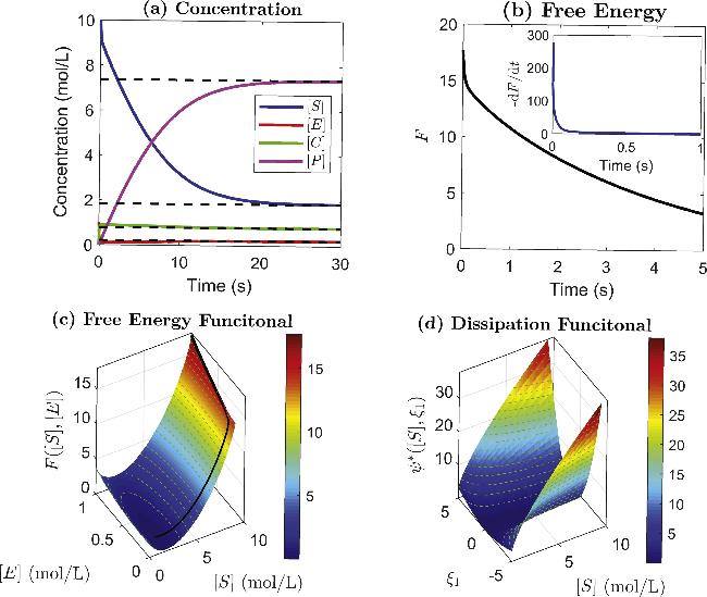
Figure 1. Dynamic and thermodynamic structures of the MM reactions. (a) The concentrations versus time of the species S, E, C, and P; the solid lines represent temporal states, while the dashed lines represent equilibrium states. (b) The free energy function F(t) and its negative gradient fd(t) (inset) versus time. (c) The free energy surface F([S], [E]) versus the concentrations [S] and [E], while the black solid line represents the trajectory from the given initial state. (d) The dissipation function ψ*([S], ξ1) versus the concentration [S] and ξ1. For all plots, the initial concentrations are ([S], [E], [C], [P])|t=0 = (10, 1, 0, 0), and the rate constants are $({\kappa }_{1}^{+},{\kappa }_{1}^{-},{\kappa }_{2}^{+},{\kappa }_{2}^{-})=(2,1,1,0.5)$. |
4.2. Diffusion equations
In the second example, we consider the classical diffusion system on a bounded smooth domain ${\rm{\Omega }}\subset {{\mathbb{R}}}^{d}$. The governing equation for the density ρ = ρ(t, x) reads
$\begin{eqnarray}{\partial }_{t}\rho (t,{\boldsymbol{x}})=D{{\rm{\Delta }}}_{{\boldsymbol{x}}}\rho ,\end{eqnarray}$
where the constant D > 0 is the diffusion coefficient. The relative entropy for this system is $\begin{eqnarray}F(\rho )={\int }_{{\rm{\Omega }}}(\rho \mathrm{ln}\rho -\rho ){\rm{d}}{\boldsymbol{x}}.\end{eqnarray}$
GCS for diffusion equations. The classical diffusion equation (47 ) obeys the GCS [33] as 48 ), and the antisymmetric operator A(c) = 0. In fact, using the relations $\frac{\partial {\psi }^{* }(\rho ,\xi )}{\partial \xi }=-{\rm{\nabla }}\cdot (D\rho {\rm{\nabla }}\xi )$ and ${{\rm{\nabla }}}_{\rho }F=\mathrm{ln}\rho $, we find $\frac{\partial {\psi }^{* }(\rho ,\xi )}{\partial \xi }{| }_{\xi =-{\rm{\nabla }}F}$ = ${\rm{\nabla }}\cdot (D\rho {\rm{\nabla }}\mathrm{ln}\rho )$ = D∆xρ.
$\begin{eqnarray}\frac{\partial \rho }{\partial t}{\left.=\frac{\partial {\psi }^{* }(\rho ,\xi )}{\partial \xi }\right|}_{\xi =-{{\rm{\nabla }}}_{\rho }F},\end{eqnarray}$
where the dissipation function ψ*(c, ξ) is defined as $\begin{eqnarray}{\psi }^{* }(\rho ,\xi )={\int }_{{\rm{\Omega }}}\frac{1}{2}D\rho | {{\rm{\nabla }}}_{{\boldsymbol{x}}}\xi {| }^{2}{\rm{d}}{\boldsymbol{x}}.\end{eqnarray}$
In the above, the relative entropy is chosen as in equation (EVA for diffusion equations. With respect to the continuity equation, 48 ), and the rate of energy dissipation as 47 ).
$\begin{eqnarray}{\partial }_{t}\rho (t,{\boldsymbol{x}})=-{{\rm{\nabla }}}_{{\boldsymbol{x}}}\cdot (\rho {\boldsymbol{v}}),\end{eqnarray}$
where v = v(t, x) denotes the velocity. Wang et al [32] showed that the diffusion equation can be obtained from the EVA. We choose the total energy of the system as Etot = F(ρ) in equation ( $\begin{eqnarray}{{\rm{\Delta }}}_{E}(\rho ;{\boldsymbol{v}})={\int }_{{\rm{\Omega }}}{D}^{-1}\rho | {\boldsymbol{v}}{| }^{2}{\rm{d}}{\boldsymbol{x}}.\end{eqnarray}$
Considering the fact that dF/dt = ‹δF/δρ, ∂tρ› and $\delta F/\delta \rho =\mathrm{ln}\rho $, the energy-dissipation law $\frac{{\rm{d}}}{{\rm{d}}t}F(\rho )=-{{\rm{\Delta }}}_{E}(\rho ;{\boldsymbol{v}})$ actually implies $\begin{eqnarray}\begin{array}{rcl}\langle \mathrm{ln}\rho ,{\partial }_{t}\rho \rangle & = & \langle \mathrm{ln}\rho ,-{{\rm{\nabla }}}_{{\boldsymbol{x}}}\cdot (\rho {\boldsymbol{v}})\rangle \\ & = & \langle \rho {\boldsymbol{v}},{{\rm{\nabla }}}_{{\boldsymbol{x}}}(\mathrm{ln}\rho )\rangle =\langle \rho {\boldsymbol{v}},-{D}^{-1}{\boldsymbol{v}}\rangle ,\end{array}\end{eqnarray}$
where in the second equality we used integration by parts and ignored the boundary terms. Based on the last equality, we can derive the constitutive relation of velocity ${\boldsymbol{v}}=-D{{\rm{\nabla }}}_{{\boldsymbol{x}}}(\mathrm{ln}\rho )$, which is recognized as Fick's law of diffusion. Direct substitution of Fick's law into the continuity equation recovers the original diffusion equation in equation (CIT for diffusion equations. The classical diffusion equation can be constructed on the basis of classical irreversible thermodynamics, too. The starting point is also the continuity equation in equation (51 ). To find a proper constitutive relation for the velocity v, we turn to the entropy function S(ρ) = [U(ρ) - F(ρ)]/T = ${\int }_{{\rm{\Omega }}}(\rho {u}_{0}-\rho \mathrm{ln}\rho $ + ρ)dx, where u0 denotes the specific internal energy. Recalling the Gibbs relation, we have
$\begin{eqnarray*}\begin{array}{rcl}\frac{{\rm{d}}S}{{\rm{d}}t} & = & \frac{1}{T}\frac{{\rm{d}}}{{\rm{d}}t}{\displaystyle \int }_{{\rm{\Omega }}}(\rho {u}_{0}-\rho \mathrm{ln}\rho +\rho ){\rm{d}}{\boldsymbol{x}}\\ & = & \frac{1}{T}{\displaystyle \int }_{{\rm{\Omega }}}\frac{\partial \rho }{\partial t}({u}_{0}-\mathrm{ln}\rho ){\rm{d}}{\boldsymbol{x}}\\ & = & -\frac{1}{T}{\displaystyle \int }_{{\rm{\Omega }}}{{\rm{\nabla }}}_{{\boldsymbol{x}}}\cdot (\rho {\boldsymbol{v}})({u}_{0}-\mathrm{ln}\rho ){\rm{d}}{\boldsymbol{x}}\\ & = & \frac{1}{T}{\displaystyle \int }_{{\rm{\Omega }}}\rho {\boldsymbol{v}}\cdot {{\rm{\nabla }}}_{{\boldsymbol{x}}}({u}_{0}-\mathrm{ln}\rho ){\rm{d}}{\boldsymbol{x}}\\ & = & \frac{1}{T}{\displaystyle \int }_{{\rm{\Omega }}}{\boldsymbol{v}}\cdot {{\rm{\nabla }}}_{{\boldsymbol{x}}}\rho {\rm{d}}{\boldsymbol{x}}={\rm{e}}{\rm{p}}{\rm{r}}\geqslant 0.\end{array}\end{eqnarray*}$
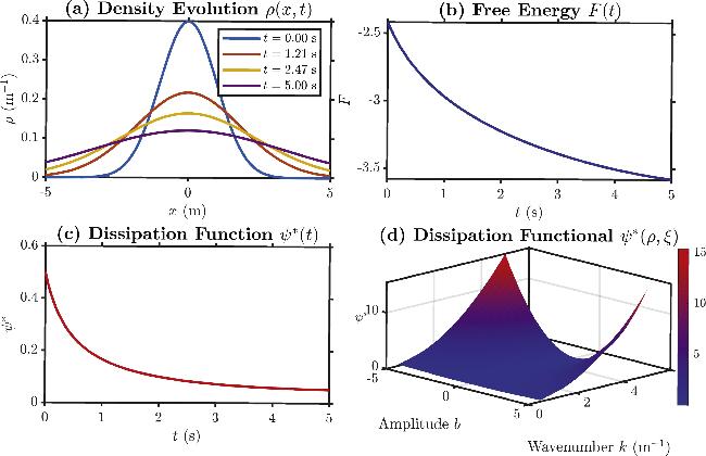
In order to keep the non-negativeness of the entropy production rate, we can take Fick's law, which in turn gives the classical diffusion equation.Numerical results on diffusion equations. In figure 2, the dynamic and thermodynamic structures of the diffusion equations are presented. Figure 2(a) shows the temporal evolution of the density profile ρ(t, x), which evolves from an initial Gaussian distribution throughout the spatial domain [-L, L] with L = 20 at t = 0 towards a uniform equilibrium state as t increases. Figures 2(b), (c) jointly demonstrate the thermodynamic consistency of the diffusion process. The free energy in (b) decreases monotonically. Meanwhile, the dissipation function ${\psi }^{* }(t)=\int \frac{1}{2}D\rho | {\rm{\nabla }}\xi {| }^{2}{\rm{d}}x$ in (c) along the path $\xi =-{{\rm{\nabla }}}_{\rho }F=-\mathrm{ln}\rho $ decays rapidly from its maximum at t = 0 to zero as the system reaches equilibrium. Figure 2(d) illustrates the dissipation functional surface ψ*(ρ, ξ) at fixed time t = 2.47, evaluated for trial functions $\xi (x)=b\cdot \sin (2\pi kx/L)$. The parabolic dependence on the amplitude b reflects the quadratic form of the dissipation functional, while the increasing curvature with the wavenumber k demonstrates the enhanced dissipation at smaller length scales.
Figure 2. Dynamic and thermodynamic structures of the diffusion equations. (a) Density profiles ρ(t, x) at four different times. (b) Temporal evolution of the free energy function $F(t)=\int (\rho {\rm{ln}}\rho -\rho )dx$. (c) Temporal evolution of the dissipation function ${\psi }^{* }(t)=\int \frac{1}{2}D\rho | {\rm{\nabla }}\xi {| }^{2}dx$ along the path $\xi =-{{\rm{\nabla }}}_{\rho }F=-{\rm{ln}}\rho $. (d) Dissipation functional surface ψ*(ρ, ξ) at fixed t = 2.47 with $\xi (x)=b\cdot {\rm{\sin }}(2\pi kx/L)$, illustrating its dependence on the amplitude b and wavenumber k. For all plots, the diffusion coefficient D = 1.0, spatial domain [-L, L] with L = 20. |
5. Conclusion and discussion
In this paper, we make a thorough revision of the GCS, which includes the Hamiltonian dynamics and the gradient system as two specific cases. We highlight the elegant mathematical properties of the generalized gradient system, including its close relation to the large deviations principle, reformulation in Wasserstein space, extension in metric spaces, as well as physical interpretation in the laws of thermodynamics. Most importantly, based on the GCS, we demonstrate a unification of various thermodynamic modeling approaches, including the GENERIC, OVP, the EVA and CIT, and suggest that they can lead to consistent results by proper formulation. Through our results, the intrinsic connections among different thermodynamic modeling approaches are clearly revealed, which sheds light on the construction of a unified theoretical framework for modeling various non-equilibrium thermodynamic processes in the future.
Though the GCS provides a very powerful framework with solid modern mathematical foundations, the classical physical systems (or models) that could be rewritten into GCS are still quite limited. A major difficulty is how to find a proper dissipation function and justify its mathematical properties as required. In addition, the separation of conservative and dissipative parts with respect to a new model is usually not straightforward. Another interesting point worthy of further exploration is the merits of GCS in data-driven modeling.