Welcome to visit Communications in Theoretical Physics,
Mathematical Physics

Double-pole soliton solutions of the defocusing nonlinear Schrödinger equation with local and nonlocal nonlinearities under nonzero boundary conditions

  • Chuanxin Xu 1 ,
  • Tao Xu , 1, * ,
  • Min Li 2 ,
  • Yuzhi Zhang 1
Expand
  • 1College of Science, China University of Petroleum, Beijing 102249, China
  • 2Department of Mathematics and Physics, North China Electric Power University, Beijing 102206, China

Author to whom any correspondence should be addressed.

Received date: 2025-08-26

  Revised date: 2025-10-12

  Accepted date: 2025-10-22

  Online published: 2025-11-26

Copyright

© 2025 Institute of Theoretical Physics CAS, Chinese Physical Society and IOP Publishing. All rights, including for text and data mining, AI training, and similar technologies, are reserved.
This article is available under the terms of the IOP-Standard License.

Abstract

Under study in this paper is a nonlinear Schrödinger equation with local and nonlocal nonlinearities, which originates from the parity-symmetric reduction of the Manakov system and has applications in some physical systems with the parity symmetry constraint between two fields/components. Via the Riemann-Hilbert method, the theory of inverse scattering transform with the presence of double poles is extended for this equation under nonzero boundary conditions (NZBCs). Also, the double-pole soliton solutions with NZBCs are derived in the reflectionless case. It is shown that the quasi-periodic beating solitons can be obtained when the double pole lies off the circle $\Gamma$ centered at the origin with radius $\sqrt{2}{q}_{0}$ (where q0 is the modulus of NZBCs) on the spectrum plane. Moreover, using the improved asymptotic analysis method, the asymptotic solitons are found to be located in some logarithmic curves of the xt plane.

Cite this article

Chuanxin Xu , Tao Xu , Min Li , Yuzhi Zhang . Double-pole soliton solutions of the defocusing nonlinear Schrödinger equation with local and nonlocal nonlinearities under nonzero boundary conditions[J]. Communications in Theoretical Physics, 2026 , 78(3) : 035001 . DOI: 10.1088/1572-9494/ae15eb

1. Introduction

As a two-component vector generalization of the scalar nonlinear Schrödinger (NLS) equation, the Manakov system is an important integrable nonlinear wave model [1]:
$\begin{eqnarray}\begin{array}{c}{\rm{i}}{q}_{t}(x,t)+{q}_{{xx}}(x,t)+2\sigma q(x,t)\\ \,\times \,[|q(x,t){|}^{2}+|r(x,t){|}^{2}]=0,\end{array}\end{eqnarray}$
$\begin{eqnarray}\begin{array}{c}{\rm{i}}{r}_{t}(x,t)+{r}_{{xx}}(x,t)+2\sigma r(x,t)\\ \,\times [|r(x,t){|}^{2}+|q(x,t){|}^{2}]=0,\end{array}\end{eqnarray}$
where x and t are, respectively, the normalized distance and time coordinates, q(x, t) and r(x, t) are the slowly varying envelopes of two copropagating waves, and σ = ±1 correspond to the focusing (+) and defocusing (-) cases, respectively. System (1.1) has significant applications in various physical settings, such as two-component Bose-Einstein condensates [2, 3], birefringent/two-mode optical fibers [4-7], a Kerr-like photorefractive medium [8] and two-wave systems in deep water [9]. Meanwhile, system (1.1) admits many remarkable integrable properties, like infinitely many set of conserved densities [1, 10, 11], closure of the product eigenstates [10], an infinite-dimensional algebra of nonlocal and noncommutative symmetries [12], Bäcklund/Darboux transformation (DT) [13-15], Painlevé properties [13] and Hirota bilinearization [16]. Additionally, system (1.1) possesses the bright-bright, dark-dark, bright-dark vector soliton solutions [16-25] and exotic vector breather and rogue-wave solutions [26-28]. On the other hand, system (1.1) can exhibit both shape-preserving and shape-changing vector-soliton collisions [16-18, 29], where the latter is accompanied by energy exchange between two components. It should be noted that the shape-changing Manakov soliton collisions have been experimentally observed in Kerr-like media and birefringent optical fibers [30, 31], potential applications in all-optical virtual logic, computation and switching [32-35].
In 2018, inspired by Ablowitz and Musslimani's work in 2013 [36], Yang considered the parity-symmetric constraint between two components of the Manakov system (i.e. r(x, t) = q(-x, t)), and proposed the following integrable nonlocal NLS equation:
$\begin{eqnarray}\begin{array}{l}{\rm{i}}{q}_{t}(x,t)+{q}_{xx}(x,t)+2\sigma q(x,t)\left[| q(x,t){| }^{2}\right.\\ \,\left.+\,| \,q(-x,t){| }^{2}\right]=0,\end{array}\end{eqnarray}$
which incorporates the local and nonlocal nonlinearities, where the combined nonlinear terms depend on x as well as -x and exhibit symmetry in x. Since equation (1.2) arises from the parity-symmetric reduction of the Manakov system (1.1), it can describe the nonlinear wave propagation in such physical systems with certain constraints on the initial conditions. Therefore, the physical significance of equation (1.2) is evident owing to its relation to the Mannakov system.
Due to the Lax pair of the Manakov system (1.1) being in the 3 × 3 matrix form, its inverse scattering transform (IST) has attracted considerable attention for a long time. In 1974, Manakov first established the IST of system (1.1) under zero boundary conditions (ZBCs) [1]. Then, Ablowitz et al extended the IST theory with ZBCs for the multi-component and matrix NLS equations [37]. The IST formulations for both the focusing and defocusing Manakov systems with nonzero boundary conditions (NZBCs) were studied, as seen, for example, in Refs. [38-41]. Furthermore, Abeya et al developed the IST of the defocusing Manakov system by considering the non-parallel boundary conditions [42] and well-defined parity-symmetric boundary conditions [43]. Recently, in the framework of the Riemann-Hilbert problem (RHP), the IST theory of equation (1.2) with ZBCs was studied by starting from the x-part [44] and the t-part [45, 46] of the Lax pair, respectively. Yang obtained the bright one- and two-soliton solutions by examining the discrete scattering symmetries in the Manakov system [44], but the intricate dependencies of eigenvector symmetry relations on eigenvalue configurations (including the number and locations) are a challenge in the construction of N-soliton solutions. By making the spectral analysis of the t-part of the Lax pair, Wu derived the N-soliton solutions of equation (1.2) with ZBCs in the reflectionless case [45, 46]. Additionally, equation (1.2) has been exactly solved by other analytic methods, such as Hirota's bilinear method [47] and DT [48].
Up to now, the existing studies on equation (1.2) have been mainly conducted under ZBCs. In [49], we firstly established the IST of the defocusing equation (1.2) under NZBCs by introducing the adjoint Lax pair and auxiliary eigenfunctions. Also, the N-soliton solutions were presented in the determinant form, and the soliton dynamical behaviors were studied based on the distribution of discrete eigenvalues and the asymptotic behaviors of solutions. It turns out that the defocusing case of equation (1.2) admits the beating and dark soliton solutions, where the former is associated with the discrete eigenvalue pairs lying off $\Gamma$ which is centered at the origin with radius $\sqrt{2}{q}_{0}$ on the spectrum plane and q0 denoting the modulus of NZBCs, while the dark solitons correspond to the discrete eigenvalue pairs lying on the circle $\Gamma$. Moreover, the solutions can exhibit abundant soliton interactions including beating-beating, dark-dark, and beating-dark types. However, [49] assumed that the reciprocals of analytic scattering coefficients admit only simple poles, omitting the possibility of higher-order poles. In the case of higher-order poles, the IST theory had already been developed for many local and nonlocal integrable models in the past several decades (e.g. see Refs. [50-57]). In this paper, we extend the IST theory of defocusing equation (1.2) under NZBCs by considering that the reciprocals of scattering coefficients have double poles. Then, we derive the double-pole soliton solutions and use the improved asymptotic analysis method [58-60] to study the dynamical properties of double-pole soliton interactions.
The outline of this work is as follows: in section 2, we review the results of the direct scattering problem, which were proved in [49]. In section 3, based on the results for the inverse problem with NZBCs, we analyze the distributions, constraints and pole contributions of discrete eigenvalues and extend the trace formulas and reconstruction formulas with the presence of double poles. In section 4, we discuss the soliton dynamical properties of double-pole soliton solutions based on the distribution of discrete eigenvalues and the asymptotic behaviors of solutions. Finally, the conclusions are presented in section 5.

2. Brief review: direct scattering problem with NZBCs

In this section, we present a short review of the direct scattering problem of equation (1.2) with NZBCs, which was studied in [49]. The results include the analyticity, symmetries and asymptotic behaviors of the Jost eigenfunctions, the adjoint Jost eigenfunctions, and the associated scattering data.

2.1. Lax pair and adjoint lax pair

We consider the NZBCs of equation (1.2) as follows:
$\begin{eqnarray}\mathop{\mathrm{lim}}\limits_{x\to \,\pm \,\infty }q(x,t)={q}_{\pm }{{\rm{e}}}^{-2{\rm{i}}(| {q}_{+}{| }^{2}+| {q}_{-}{| }^{2})t},\end{eqnarray}$
where q ± ≠ 0 are independent of x and t. To eliminate the t-dependence in boundary conditions, we make the transformation $q(x,t)\to \hat{q}(x,t){{\rm{e}}}^{-2{\rm{i}}(| {q}_{+}{| }^{2}+| {q}_{-}{| }^{2})t}$ and present the following nonzero boundary-value problem:
$\begin{eqnarray}\begin{array}{l}{\rm{i}}{q}_{t}(x,t)+{q}_{xx}(x,t)-2q(x,t)\\ \quad \times \,\left(| q(x,t){| }^{2}+| q(-x,t){| }^{2}-2{q}_{0}^{2}\right)=0,\end{array}\end{eqnarray}$
$\begin{eqnarray}\mathop{\mathrm{lim}}\limits_{x\to \pm \infty }q(x,t)={q}_{\pm },\end{eqnarray}$
where ${q}_{0}^{2}=(| {q}_{+}{| }^{2}+| {q}_{-}{| }^{2})/2$ with q0 > 0, and the hat has been dropped for simplicity. Obviously, the solutions of equation (1.2) can be derived from those of equation (2.2a) through the transformation $q(x,t)=\hat{q}(x,t){{\rm{e}}}^{-4{\rm{i}}{q}_{0}^{2}t}$.
Equation (2.2a) is associated with the following Zakharov-Shabat scattering problem:
$\begin{eqnarray}\begin{array}{l}{{\boldsymbol{\phi }}}_{x}(x,t,k)={\boldsymbol{X}}(x,t,k){\boldsymbol{\phi }}(x,t,k),\\ {\boldsymbol{X}}(x,t,k)=-{\rm{i}}k{{\boldsymbol{\sigma }}}_{3}+{\boldsymbol{Q}},\end{array}\end{eqnarray}$
$\begin{eqnarray}\begin{array}{l}{{\boldsymbol{\phi }}}_{t}(x,t,k)={\boldsymbol{T}}(x,t,k){\boldsymbol{\phi }}(x,t,k),\\ {\boldsymbol{T}}(x,t,k)=2k{\boldsymbol{X}}+{\rm{i}}{{\boldsymbol{\sigma }}}_{3}{{\boldsymbol{Q}}}_{x}-{\rm{i}}{{\boldsymbol{\sigma }}}_{3}{{\boldsymbol{Q}}}^{2}-{{\boldsymbol{V}}}_{0},\end{array}\end{eqnarray}$
with
$\begin{eqnarray}\begin{array}{l}{{\boldsymbol{\sigma }}}_{3}=\left(\begin{array}{rcl}1 & 0 & 0\\ 0 & 1 & 0\\ 0 & 0 & -1\\ & & \end{array}\right),\\ {\boldsymbol{Q}}=\left(\begin{array}{rcl}0 & 0 & q(x,t)\\ 0 & 0 & q(-x,t)\\ {q}^{* }(x,t) & {q}^{* }(-x,t) & 0\\ & & \end{array}\right),\\ {{\boldsymbol{V}}}_{0}=\left(\begin{array}{rcl}-2{\rm{i}}{q}_{0}^{2} & 0 & 0\\ 0 & -2{\rm{i}}{q}_{0}^{2} & 0\\ 0 & 0 & 2{\rm{i}}{q}_{0}^{2}\\ & & \end{array}\right),\end{array}\end{eqnarray}$
where Φ(x, t, k) is the 3 × 3 matrix solution, k is the complex spectral parameter and '*' represents complex conjugate.
Subject to the boundary condition (2.2b), the limits of matrices X and T can be given by
$\begin{eqnarray}{{\boldsymbol{X}}}_{\pm }(k)=\left(\begin{array}{ccc}-{\rm{i}}k & 0 & {q}_{\pm }\\ 0 & -{\rm{i}}k & {q}_{\mp }\\ {q}_{\pm }^{* } & {q}_{\mp }^{* } & {\rm{i}}k\\ \end{array}\right),\end{eqnarray}$
$\begin{eqnarray}{{\boldsymbol{T}}}_{\pm }(k)=\left(\begin{array}{ccc}-{\rm{i}}| {q}_{\pm }{| }^{2}-2{\rm{i}}{k}^{2}+2{\rm{i}}{q}_{0}^{2} & -{\rm{i}}{q}_{\pm }{q}_{\mp }^{* } & 2k{q}_{\pm }\\ -{\rm{i}}{q}_{\mp }{q}_{\pm }^{* } & -{\rm{i}}| {q}_{\mp }{| }^{2}-2{\rm{i}}{k}^{2}+2{\rm{i}}{q}_{0}^{2} & 2k{q}_{\mp }\\ 2k{q}_{\pm }^{* } & 2k{q}_{\mp }^{* } & 2{\rm{i}}{k}^{2}\\ \end{array}\right),\end{eqnarray}$
which possess the eigenvalues as follows:
$\begin{eqnarray}\begin{array}{l}{{\boldsymbol{X}}}_{\pm }:\{-{\rm{i}}k,\,\pm {\rm{i}}\lambda \},\quad {{\boldsymbol{T}}}_{\pm }:\{-2{\rm{i}}{k}^{2}+2{\rm{i}}{q}_{0}^{2},\,\pm 2{\rm{i}}k\lambda \}\\ \quad \,\rm{with}\,\,\,\lambda (k)=\sqrt{{k}^{2}-2{q}_{0}^{2}}.\end{array}\end{eqnarray}$
Considering the branching for λ(k) in the complex k-plane, we introduce the uniformization variable z = k + λ(k). From the relations $k=\frac{1}{2}\left(z+\frac{2{q}_{0}^{2}}{z}\right)$ and $\lambda =\frac{1}{2}\left(z-\frac{2{q}_{0}^{2}}{z}\right)$, the eigenvalues of X ± and T ± can be rewritten as follows:
$\begin{eqnarray}\begin{array}{l}{{\boldsymbol{X}}}_{\pm }:\left\{-\frac{{\rm{i}}}{2}\left(z+\frac{2{q}_{0}^{2}}{z}\right),\pm \frac{{\rm{i}}}{2}\left(z-\frac{2{q}_{0}^{2}}{z}\right)\right\},\\ {{\boldsymbol{T}}}_{\pm }:\left\{-\frac{{\rm{i}}}{2}{\left(z+\frac{2{q}_{0}^{2}}{z}\right)}^{2}+2{\rm{i}}{q}_{0}^{2},\pm \frac{{\rm{i}}}{2}\left({z}^{2}-\frac{4{q}_{0}^{4}}{{z}^{2}}\right)\right\}.\end{array}\end{eqnarray}$
Also, the common eigenvector matrices of X ± and T ± are presented as
$\begin{eqnarray}{{\boldsymbol{Y}}}_{\pm }=\left(\begin{array}{ccc}\frac{{q}_{\pm }}{{q}_{0}} & -\frac{{q}_{\mp }^{* }}{\sqrt{2}{q}_{0}} & \frac{-{\rm{i}}\sqrt{2}{q}_{\pm }}{z}\\ \frac{{q}_{\mp }}{{q}_{0}} & \frac{{q}_{\pm }^{* }}{\sqrt{2}{q}_{0}} & \frac{-{\rm{i}}\sqrt{2}{q}_{\mp }}{z}\\ \frac{2{\rm{i}}{q}_{0}}{z} & 0 & \sqrt{2}\\ \end{array}\right)\end{eqnarray}$
with the determinant ${\rm{\det }}({{\boldsymbol{Y}}}_{\pm }):= \gamma (z)=2-4{q}_{0}^{2}/{z}^{2}$.
The 3 × 3 matrix solutions Φ ± (x, t, z) of equation (2.3a) satisfy the following Volterra integral equations:
$\begin{eqnarray}\begin{array}{l}{{\boldsymbol{\phi }}}_{-}(x,t,z)={{\boldsymbol{Y}}}_{-}(z){\boldsymbol{E}}(x,t,z)\\ \quad +\,{\int }_{-\infty }^{x}{{\boldsymbol{Y}}}_{-}(z){{\rm{e}}}^{{\rm{i}}{\boldsymbol{J}}(z)(x-y)}{{\boldsymbol{Y}}}_{-}^{-1}(z)\\ \quad \times \,{\boldsymbol{\Delta }}{{\boldsymbol{Q}}}_{-}(y,t){{\boldsymbol{\phi }}}_{-}(y,t,z){\rm{d}}y,\end{array}\end{eqnarray}$
$\begin{eqnarray}\begin{array}{l}{{\boldsymbol{\phi }}}_{+}(x,t,z)={{\boldsymbol{Y}}}_{+}(z){\boldsymbol{E}}(x,t,z)\\ \quad -\,{\displaystyle \int }_{x}^{\infty }{{\boldsymbol{Y}}}_{+}(z){{\rm{e}}}^{{\rm{i}}{\boldsymbol{J}}(z)(x-y)}{{\boldsymbol{Y}}}_{+}^{-1}(z)\\ \quad \times \,{\boldsymbol{\Delta }}{{\boldsymbol{Q}}}_{+}(y,t){{\boldsymbol{\phi }}}_{+}(y,t,z){\rm{d}}y,\end{array}\end{eqnarray}$
where J(z) = diag( - λ, k, λ), Q ± (x, t) := Q(x, t) - Q ± and ${{\boldsymbol{Q}}}_{\pm }=\mathop{\mathrm{lim}}\limits_{x\to \pm \infty }{\boldsymbol{Q}}(x,t)$. The functions Φ ± are called the Jost eigenfunctions and can exhibit the asymptotic behaviors
$\begin{eqnarray}{{\boldsymbol{\phi }}}_{\pm }(x,t,z)\sim {{\boldsymbol{Y}}}_{\pm }(z){\boldsymbol{E}}(x,t,z)+o(1),\quad x\to \pm \infty ,\end{eqnarray}$
where
$\begin{eqnarray}\begin{array}{l}{\boldsymbol{E}}(x,t,z)={{\rm{e}}}^{{\rm{i}}{\boldsymbol{\Theta }}(x,t,z)},\\ {\boldsymbol{\Theta }}(x,t,z)=\mathrm{diag}[{\theta }_{1}(x,t,z),{\theta }_{2}(x,t,z),-{\theta }_{1}(x,t,z)],\\ {\theta }_{1}(x,t,z)=-\lambda x-2k\lambda t,\\ {\theta }_{2}(x,t,z)=-kx-2({k}^{2}-{q}_{0}^{2})t.\end{array}\end{eqnarray}$
Meanwhile, to factorize the exponential oscillations, we use the modified Jost eigenfunctions
$\begin{eqnarray}{{\boldsymbol{\mu }}}_{\pm }(x,t,z)={{\boldsymbol{\phi }}}_{\pm }(x,t,z){{\boldsymbol{E}}}^{-1}(x,t,z),\end{eqnarray}$
so that $\mathop{\mathrm{lim}}\limits_{x\to \pm \infty }{{\boldsymbol{\mu }}}_{\pm }(x,t,z)={{\boldsymbol{Y}}}_{\pm }(z)$.
Also, we introduce the 3 × 3 scattering matrix A(z) = (aij(z)) which relates the solutions Φ ± of equation (2.3a):
$\begin{eqnarray}\begin{array}{l}{{\boldsymbol{\phi }}}_{-}(x,t,z)={{\boldsymbol{\phi }}}_{+}(x,t,z){\boldsymbol{A}}(z),\\ \quad z\in {{\rm{\Sigma }}}_{o}:\,{\mathbb{R}}\setminus \{\pm \sqrt{2}{q}_{0}\},\end{array}\end{eqnarray}$
and define its inverse A-1(z) = B(z) = (bij(z)). Here, it can be determined that ${\rm{\det }}({{\boldsymbol{\phi }}}_{\pm }(x,t,z))=\gamma (z){{\rm{e}}}^{{\rm{i}}{\theta }_{2}(x,t,z)}$ and ${\rm{\det }}({\boldsymbol{A}}(z))=1$ for z ∈ Σo.
Let ${C}^{+}=\{z\in {\mathbb{C}}| {\rm{Im}}(z)\gt 0\}$ and C- = $\{z\in {\mathbb{C}}| {\rm{Im}}(z)\lt 0\}$. As proved in [49] (see theorems 2.1 and 2.2 there), μ-,1(x, t, z), μ+,3(x, t, z), a11(z), b33(z) are analytic for zC+, while μ+,1(x, t, z), μ-,3(x, t, z), a33(z), b11(z) are analytic for zC-, where the subscripts of μ± ,i denote the ith columns of μ ±. Based on the relation (2.12), the corresponding columns of Φ ± (x, t, z) possess the same analyticity. However, μ ± ,2(x, t, z) (or Φ ± ,2(x, t, z)) and the remaining entries of A(z) and B(z) are nowhere analytic in general.
On the other hand, it is necessary to introduce the adjoint Lax pair [38-40]:
$\begin{eqnarray}\begin{array}{l}{\tilde{{\boldsymbol{\phi }}}}_{x}(x,t,k)=\tilde{{\boldsymbol{X}}}(x,t,k){\boldsymbol{\phi }}(x,t,k),\\ {\tilde{{\boldsymbol{\phi }}}}_{t}(x,t,k)=\tilde{{\boldsymbol{T}}}(x,t,k){\boldsymbol{\phi }}(x,t,k),\end{array}\end{eqnarray}$
with
$\begin{eqnarray}\tilde{{\boldsymbol{X}}}(x,t,k)={{\boldsymbol{X}}}^{* }(x,t,{k}^{* })={\rm{i}}k{{\boldsymbol{\sigma }}}_{3}+{{\boldsymbol{Q}}}^{* }(x,t),\end{eqnarray}$
$\begin{eqnarray}\begin{array}{l}\tilde{{\boldsymbol{T}}}(x,t,k)={{\boldsymbol{T}}}^{* }(x,t,{k}^{* })=2k\tilde{{\boldsymbol{X}}}(x,t,k)\\ \quad -\,{\rm{i}}{{\boldsymbol{\sigma }}}_{3}{{\boldsymbol{Q}}}_{x}^{* }(x,t)+{\rm{i}}{{\boldsymbol{\sigma }}}_{3}{({{\boldsymbol{Q}}}^{* })}^{2}(x,t)+{{\boldsymbol{V}}}_{0}.\end{array}\end{eqnarray}$
Similarly, for the matrix limits ${\tilde{{\boldsymbol{X}}}}_{\pm }(k)=\mathop{\mathrm{lim}}\limits_{x\to \pm \infty }\tilde{{\boldsymbol{X}}}(x,t,k)$ and ${\tilde{{\boldsymbol{T}}}}_{\pm }(k)=\mathop{\mathrm{lim}}\limits_{x\to \pm \infty }\tilde{{\boldsymbol{T}}}(x,t,k)$, their eigenvalues can be given by {ik, ± iλ} and $\{2{\rm{i}}{k}^{2}-2{\rm{i}}{q}_{0}^{2}$, ± 2i}, respectively. By the uniformization variable z = k + λ(k), the common eigenvector matrices are presented below:
$\begin{eqnarray}{\tilde{{\boldsymbol{Y}}}}_{\pm }(z)={{\boldsymbol{Y}}}_{\pm }^{* }({z}^{* })=\left(\begin{array}{ccc}\frac{{q}_{\pm }^{* }}{{q}_{0}} & -\frac{{q}_{\mp }}{\sqrt{2}{q}_{0}} & \frac{{\rm{i}}\sqrt{2}{q}_{\pm }^{* }}{z}\\ \frac{{q}_{\mp }^{* }}{{q}_{0}} & \frac{{q}_{\pm }}{\sqrt{2}{q}_{0}} & \frac{{\rm{i}}\sqrt{2}{q}_{\mp }^{* }}{z}\\ \frac{-2{\rm{i}}{q}_{0}}{z} & 0 & \sqrt{2}\\ \end{array}\right),\end{eqnarray}$
where the determinant of ${\tilde{{\boldsymbol{Y}}}}_{\pm }(z)$ is $\gamma$(z). Meanwhile, the adjoint Jost eigenfunctions ${\tilde{{\boldsymbol{\phi }}}}_{\pm }(x,t,z)$ and the modified adjoint Jost eigenfunctions ${\tilde{{\boldsymbol{\mu }}}}_{\pm }(x,t,z)$ are introduced and they satisfy the asymptotic behaviors:
$\begin{eqnarray}\begin{array}{l}{\tilde{{\boldsymbol{\phi }}}}_{\pm }(x,t,z)\sim {\tilde{{\boldsymbol{Y}}}}_{\pm }(z){{\boldsymbol{E}}}^{-1}(x,t,z)\\ \quad +\,o(1),\,x\to \pm \infty ,\\ {\tilde{{\boldsymbol{\mu }}}}_{\pm }(x,t,z)\sim {\tilde{{\boldsymbol{Y}}}}_{\pm }(z)+o(1),\,x\to \pm \infty .\end{array}\end{eqnarray}$
Again, there exists an adjoint scattering matrix $\tilde{{\boldsymbol{A}}}(z)$ and its inverse matrix $\tilde{{\boldsymbol{B}}}(z)$ such that
$\begin{eqnarray}\begin{array}{l}{\tilde{{\boldsymbol{\phi }}}}_{-}(x,t,z)={\tilde{{\boldsymbol{\phi }}}}_{+}(x,t,z)\tilde{{\boldsymbol{A}}}(z),\\ {\tilde{{\boldsymbol{\phi }}}}_{+}(x,t,z)={\tilde{{\boldsymbol{\phi }}}}_{-}(x,t,z)\tilde{{\boldsymbol{B}}\,}(z)\,{,}z\in {{\rm{\Sigma }}}_{o},\end{array}\end{eqnarray}$
with $\tilde{{\boldsymbol{A}}}(z)=({\tilde{a}}_{ij}(z))$ and $\tilde{{\boldsymbol{B}}}(z)={\tilde{{\boldsymbol{A}}}}^{-1}(z)=({\tilde{b}}_{ij}(z))$.
Referring to theorem 2.3a in [49], ${\tilde{{\boldsymbol{\mu }}}}_{-,1}(x,t,z),{\tilde{{\boldsymbol{\mu }}}}_{+,3}(x,t,z),{\tilde{a}}_{11}(z),{\tilde{b}}_{33}(z)$ are analytic for zC-, while ${\tilde{{\boldsymbol{\mu }}}}_{+,1}(x,t,z),{\tilde{{\boldsymbol{\mu }}}}_{-,3}(x,t,z),{\tilde{a}}_{33}(z),{\tilde{b}}_{11}(z)$ are analytic for zC+. Following Refs. [38-40], one can construct two new analytic solutions of the original Lax pair (2.3a):
$\begin{eqnarray}\begin{array}{l}{\boldsymbol{w}}(x,t,z)={{\rm{e}}}^{{\rm{i}}{\theta }_{2}(x,t,z)}{{\boldsymbol{\sigma }}}_{3}\left[{\tilde{{\boldsymbol{\phi }}}}_{-,3}(x,t,z)\right.\\ \quad \left.\times \,{\tilde{{\boldsymbol{\phi }}}}_{+,1}(x,t,z)\right]/\gamma (z),\\ \bar{{\boldsymbol{w}}}(x,t,z)={{\rm{e}}}^{{\rm{i}}{\theta }_{2}(x,t,z)}{{\boldsymbol{\sigma }}}_{3}\left[{\tilde{{\boldsymbol{\phi }}}}_{-,1}(x,t,z)\right.\\ \quad \left.\times {\tilde{{\boldsymbol{\phi }}}}_{+,3}(x,t,z)\right]/\gamma (z),\end{array}\end{eqnarray}$
where the auxiliary eigenfunctions w(x, t, z) and $\overline{{\boldsymbol{w}}}(x,t,z)$ are analytic in C+ and C-, respectively [49]. Again, to eliminate the exponential oscillation, we define the modified auxiliary eigenfunctions as follows:
$\begin{eqnarray}\begin{array}{l}{\boldsymbol{m}}(x,t,z)={\boldsymbol{w}}(x,t,z){{\rm{e}}}^{-{\rm{i}}{\theta }_{2}(x,t,z)},\\ \bar{{\boldsymbol{m}}}(x,t,z)=\bar{{\boldsymbol{w}}}(x,t,z){{\rm{e}}}^{-{\rm{i}}{\theta }_{2}(x,t,z)}.\end{array}\end{eqnarray}$

2.2. Symmetries and asymptotic behaviors

For convenience, we use a prime to denote the (partial) derivative of a given function with respect to z, for example, ${{\boldsymbol{\phi }}}_{\pm }^{{\prime} }(x,t,z)=\frac{\partial {{\boldsymbol{\phi }}}_{\pm }(x,t,z)}{\partial z}$ and ${{\boldsymbol{A}}}^{{\prime} }(z)=\frac{{\rm{d}}{\boldsymbol{A}}(z)}{{\rm{d}}z}$. Considering the mappings z $\subset$ z*, z $\subset$ -z and $z\mapsto \hat{z}\,:=\,\frac{2{q}_{0}^{2}}{z}$, [49] obtained the symmetries (see lemmas 2.8-2.13 there) of the eigenfunctions, auxiliary eigenfunctions and scattering matrices. On this basis, we further present the symmetry properties of the z-derivatives of the eigenfunctions, auxiliary eigenfunctions and scattering matrices.

The z-derivatives of Jost functions Φ ± and scattering matrices A(z) and B(z) have the following symmetries:

(1) The first symmetry (z $\subset$ z*)

$\begin{eqnarray}\begin{array}{l}{[{{\boldsymbol{\phi }}}_{\pm }^{\dagger }(x,t,{z}^{* })]}^{{\prime} }{{\boldsymbol{\sigma }}}_{3}{{\boldsymbol{\phi }}}_{\pm }(x,t,z)\\ \quad +\,{{\boldsymbol{\phi }}}_{\pm }^{\dagger }(x,t,{z}^{* }){{\boldsymbol{\sigma }}}_{3}{{\boldsymbol{\phi }}}_{\pm }^{{\prime} }(x,t,z)={{\boldsymbol{C}}}^{{\prime} }(z),\end{array}\end{eqnarray}$
$\begin{eqnarray}\begin{array}{l}{{\boldsymbol{C}}}^{{\prime} }(z){\boldsymbol{A}}(z)+{\boldsymbol{C}}(z){{\boldsymbol{A}}}^{{\prime} }(z)={[{{\boldsymbol{B}}}^{\dagger }({z}^{* })]}^{{\prime} }{\boldsymbol{C}}(z)\\ \quad +\,{{\boldsymbol{B}}}^{\dagger }({z}^{* }){{\boldsymbol{C}}}^{{\prime} }(z),\quad z\in {{\rm{\Sigma }}}_{o},\end{array}\end{eqnarray}$
where C(z) = diag($\gamma$(z), 1, -$\gamma$(z)).

(2) The second symmetry (z $\text { ↦ }$ -z)

$\begin{eqnarray}{{\boldsymbol{\phi }}}_{\pm }^{{\prime} }(x,t,z)=-{{\boldsymbol{\delta }}}_{1}{{\boldsymbol{\phi }}}_{\mp }^{{\prime} }(-x,t,-z){{\boldsymbol{\sigma }}}_{4},\end{eqnarray}$
$\begin{eqnarray}{{\boldsymbol{A}}}^{{\prime} }(z)=-{{\boldsymbol{\sigma }}}_{4}{{\boldsymbol{B}}}^{{\prime} }(-z){{\boldsymbol{\sigma }}}_{4},\quad z\in {{\rm{\Sigma }}}_{o},\end{eqnarray}$
where ${{\boldsymbol{\sigma }}}_{4}=\left(\begin{array}{ccc}1 & 0 & 0\\ 0 & -1 & 0\\ 0 & 0 & -1\\ \end{array}\right)$ and ${{\boldsymbol{\delta }}}_{1}=\left(\begin{array}{ccc}0 & 1 & 0\\ 1 & 0 & 0\\ 0 & 0 & -1\\ \end{array}\right)$.

(3) The third symmetry $(z\mapsto \hat{z})$

$\begin{eqnarray}\begin{array}{l}{{\boldsymbol{\phi }}}_{\pm }^{{\prime} }(x,t,z)=-\frac{2{q}_{0}^{2}}{{z}^{2}}{{\boldsymbol{\phi }}}_{\pm }^{{\prime} }(x,t,\hat{z}){\boldsymbol{\Pi }}(z)\\ \quad +\,{{\boldsymbol{\phi }}}_{\pm }(x,t,\hat{z}){{\boldsymbol{\Pi }}}^{{\prime} }(z),\end{array}\end{eqnarray}$
$\begin{eqnarray}\begin{array}{l}{{\boldsymbol{\Pi }}}^{{\prime} }(z){\boldsymbol{A}}(z)+{\boldsymbol{\Pi }}(z){{\boldsymbol{A}}}^{{\prime} }(z)\\ \quad =-\frac{2{q}_{0}^{2}}{{z}^{2}}{{\boldsymbol{A}}}^{{\prime} }(\hat{z}){\boldsymbol{\Pi }}(z)+{\boldsymbol{A}}(\hat{z}){{\boldsymbol{\Pi }}}^{{\prime} }(z),\quad z\in {{\rm{\Sigma }}}_{o},\end{array}\end{eqnarray}$
where ${\boldsymbol{\Pi }}(z)=\left(\begin{array}{ccc}0 & 0 & -{\rm{i}}\frac{\sqrt{2}{q}_{0}}{z}\\ 0 & 1 & 0\\ {\rm{i}}\frac{\sqrt{2}{q}_{0}}{z} & 0 & 0\\ \end{array}\right)$.

The z-derivatives of auxiliary eigenfunctions satisfy the symmetries:

$\begin{eqnarray}\begin{array}{l}{{\boldsymbol{w}}}^{{\prime} }(x,t,z)=-{{\boldsymbol{\delta }}}_{1}{\bar{{\boldsymbol{w}}}}^{{\prime} }(-x,t,-z),\\ {{\boldsymbol{w}}}^{{\prime} }(x,t,z)=\displaystyle \frac{2{q}_{0}^{2}}{{z}^{2}}{\bar{{\boldsymbol{w}}}}^{{\prime} }(x,t,\hat{z}),\quad z\in {C}^{+}.\end{array}\end{eqnarray}$

On the other hand, the asymptotic behaviors of the modified eigenfunctions, modified auxiliary eigenfunctions and scattering matrices were presented in lemma 3.3 and corollaries 3.4 and 3.5 of [49].

3. Inverse scattering problem with NZBCs

In [49], the inverse problem of defocusing equation (1.2) with NZBCs was studied by considering multiple simple poles. In this section, we will extend the results for the inverse problem with the presence of double poles, which include the properties of eigenfunctions, pole contributions, extended trace formulas and reconstruction formulas.

3.1. Distribution of discrete spectrum

For convenience, we use $\Gamma$ to represent the circle centered at the origin with radius $\sqrt{2}{q}_{0}$ in the complex z-plane. Noticing that a11(z) is analytic in C+ and satisfies a11(z) = b11(-z) and ${a}_{11}(z)={b}_{11}^{* }({z}^{* })$, we have ${a}_{11}^{{\prime} }(z)=-{b}_{11}^{{\prime} }(-z)$, ${a}_{11}^{{\prime} }(z)\,={[{b}_{11}^{{\prime} }({z}^{* })]}^{* }$. Then, we can suppose that a11(z) has
$\begin{eqnarray}\,\rm{simple zeros}:{\{{\xi }_{1,i},-{\xi }_{1,i}^{* }\}}_{i=1}^{{n}_{1}},\quad {\{{z}_{1,i},-{z}_{1,i}^{* }\}}_{i=1}^{{n}_{2}},\end{eqnarray}$
$\begin{eqnarray}\,\rm{double zeros}:{\{{\xi }_{2,i},-{\xi }_{2,i}^{* }\}}_{i=1}^{{n}_{3}},\quad {\{{z}_{2,i},-{z}_{2,i}^{* }\}}_{i=1}^{{n}_{4}},\end{eqnarray}$
where ξ1,i and ξ2,i lie on the upper half circle $\Gamma$+, and z1,i and z2,i are in C+ but off $\Gamma$+, i.e.
$\begin{eqnarray}| {\xi }_{1,i}| =| {\xi }_{2,i}| =\sqrt{2}{q}_{0},\quad | {z}_{1,i}| ,| {z}_{2,i}| \ne \sqrt{2}{q}_{0}.\end{eqnarray}$
In addition, based on the symmetries ${a}_{11}(z)=\,{a}_{33}(\hat{z}),{a}_{33}(z)\,=\,{b}_{33}(-z)$ and ${a}_{33}(z)=\,{b}_{33}^{* }({z}^{* })$, we know that ${a}_{11}^{{\prime} }(z)\,=-\frac{2{q}_{0}^{2}}{{z}^{2}}{a}_{33}^{{\prime} }(\hat{z})$, ${a}_{33}^{{\prime} }(z)=\,-{b}_{33}^{{\prime} }(-z)$ and ${a}_{33}^{{\prime} }(z)=\,{[{b}_{33}^{{\prime} }({z}^{* })]}^{* }$. So, the corresponding simple and double zeros of a33(z), b11(z) and b33(z) can also be found.

3.2. Behaviors of the eigenfunctions at the double poles

In [49], the behaviors of the eigenfunctions at simple poles were showed in lemmas 3.1 and 3.2. Referring to the proof provided in appendix B there, we can derive the behaviors of the eigenfunctions at double poles as follows:

The auxiliary eigenfunctions w at $z={\xi }_{2,i},-{\xi }_{2,i}^{* }$ and $\overline{w}$ at $z={\xi }_{2,i}^{* },-{\xi }_{2,i}$ satisfy

$\begin{eqnarray}\begin{array}{l}{\boldsymbol{w}}(x,t,{\xi }_{2,i})={\boldsymbol{w}}(x,t,-{\xi }_{2,i}^{* })\\ \quad =\,\bar{{\boldsymbol{w}}}(x,t,-{\xi }_{2,i})=\bar{{\boldsymbol{w}}}(x,t,{\xi }_{2,i}^{* })=0,\\ {{\boldsymbol{w}}}^{{\prime} }(x,t,{\xi }_{2,i})={{\boldsymbol{w}}}^{{\prime} }(x,t,-{\xi }_{2,i}^{* })\\ \quad =\,{\bar{{\boldsymbol{w}}}}^{{\prime} }(x,t,-{\xi }_{2,i})={\bar{{\boldsymbol{w}}}}^{{\prime} }(x,t,{\xi }_{2,i}^{* })=0.\end{array}\end{eqnarray}$
The Jost eigenfunctions Φ-,1 at $z={\xi }_{2,i},-{\xi }_{2,i}^{* }$ and Φ+,1 at $z={\xi }_{2,i}^{* },-{\xi }_{2,i}$ satisfy
$\begin{eqnarray}\begin{array}{l}{{\boldsymbol{\phi }}}_{-,1}(x,t,{\xi }_{2,i})={c}_{2,i}{{\boldsymbol{\phi }}}_{+,3}(x,t,{\xi }_{2,i}),\\ {{\boldsymbol{\phi }}}_{+,1}(x,t,{\xi }_{2,i}^{* })={\bar{c}}_{2,i}{{\boldsymbol{\phi }}}_{-,3}(x,t,{\xi }_{2,i}^{* }),\end{array}\end{eqnarray}$
$\begin{eqnarray}\begin{array}{l}{{\boldsymbol{\phi }}}_{+,1}(x,t,-{\xi }_{2,i})=-{c}_{2,i}{{\boldsymbol{\phi }}}_{-,3}(x,t,-{\xi }_{2,i}),\\ {{\boldsymbol{\phi }}}_{-,1}(x,t,-{\xi }_{2,i}^{* })=-{\bar{c}}_{2,i}{{\boldsymbol{\phi }}}_{+,3}(x,t,-{\xi }_{2,i}^{* }),\end{array}\end{eqnarray}$
where the norming constants c2,i and ${\bar{c}}_{2,i}$ obey the constraints:
$\begin{eqnarray}{c}_{2,i}{\bar{c}}_{2,i}=-1,\quad {\bar{c}}_{2,i}{c}_{2,i}^{* }\frac{{a}_{33}^{{\prime\prime} }({\xi }_{2,i}^{* })}{{b}_{11}^{{\prime\prime} }({\xi }_{2,i}^{* })}=1.\end{eqnarray}$
The derivatives of Jost eigenfunctions Φ-,1 at $z={\xi }_{2,i},-{\xi }_{2,i}^{* }$ and Φ+,1 at $z={\xi }_{2,i}^{* },-{\xi }_{2,i}$ satisfy
$\begin{eqnarray}\begin{array}{l}{{\boldsymbol{\phi }}}_{-,1}^{{\prime} }(x,t,{\xi }_{2,i})={c}_{2,i}{{\boldsymbol{\phi }}}_{+,3}^{{\prime} }(x,t,{\xi }_{2,i})\\ \quad +\,{h}_{2,i}{{\boldsymbol{\phi }}}_{+,3}(x,t,{\xi }_{2,i}),\end{array}\end{eqnarray}$
$\begin{eqnarray}\begin{array}{l}{{\boldsymbol{\phi }}}_{+,1}^{{\prime} }(x,t,{\xi }_{2,i}^{* })={\bar{c}}_{2,i}{{\boldsymbol{\phi }}}_{-,3}^{{\prime} }(x,t,{\xi }_{2,i}^{* })\\ \quad +\,{\bar{h}}_{2,i}{{\boldsymbol{\phi }}}_{-,3}(x,t,{\xi }_{2,i}^{* }),\end{array}\end{eqnarray}$
$\begin{eqnarray}\begin{array}{l}{{\boldsymbol{\phi }}}_{+,1}^{{\prime} }(x,t,-{\xi }_{2,i})=-{c}_{2,i}{{\boldsymbol{\phi }}}_{-,3}^{{\prime} }(x,t,-{\xi }_{2,i})\\ \quad +\,{h}_{2,i}{{\boldsymbol{\phi }}}_{-,3}(x,t,-{\xi }_{2,i}),\end{array}\end{eqnarray}$
$\begin{eqnarray}\begin{array}{l}{{\boldsymbol{\phi }}}_{-,1}^{{\prime} }(x,t,-{\xi }_{2,i}^{* })=-{\bar{c}}_{2,i}{{\boldsymbol{\phi }}}_{+,3}^{{\prime} }(x,t,-{\xi }_{2,i}^{* })\\ \quad +\,{\bar{h}}_{2,i}{{\boldsymbol{\phi }}}_{+,3}(x,t,-{\xi }_{2,i}^{* }),\end{array}\end{eqnarray}$
where the norming constants h2,i and ${\bar{h}}_{2,i}$ obey the constraints:
$\begin{eqnarray}\begin{array}{l}\displaystyle \frac{{\bar{h}}_{2,i}}{{h}_{2,i}}=-\displaystyle \frac{{\xi }_{2,i}^{2}}{2{q}_{0}^{2}}{\bar{c}}_{2,i}^{2},\\ \displaystyle \frac{{\bar{h}}_{2,i}}{{\bar{c}}_{2,i}}+\displaystyle \frac{{h}_{2,i}^{\ast }}{{c}_{2,i}^{\ast }}=-\displaystyle \frac{{b}_{11}^{{\rm{{\prime\prime} }}}({\xi }_{2,i}^{\ast })}{3{a}_{33}^{{\rm{{\prime\prime} }}}({\xi }_{2,i}^{\ast })}{\left[\displaystyle \frac{{a}_{33}^{{\rm{{\prime\prime} }}}(z)}{{b}_{11}^{{\rm{{\prime\prime} }}}(z)}\right]}_{z={\xi }_{2,i}^{\ast }}^{{\rm{{\prime} }}}.\end{array}\end{eqnarray}$

The auxiliary eigenfunctions w at $z\,={z}_{2,i},-{z}_{2,i}^{* },-{\hat{z}}_{2,i},{\hat{z}}_{2,i}^{* }$ and $\overline{w}$ at $z=-{z}_{2,i},{z}_{2,i}^{* },{\hat{z}}_{2,i},-{\hat{z}}_{2,i}^{* }$ satisfy the following relations:

$\begin{eqnarray}\begin{array}{l}{\boldsymbol{w}}(x,t,{z}_{2,i})={d}_{2,i}{{\boldsymbol{\phi }}}_{-,1}(x,t,{z}_{2,i}),\\ {\boldsymbol{w}}(x,t,-{z}_{2,i}^{* })={\breve{d}}_{2,i}{{\boldsymbol{\phi }}}_{-,1}(x,t,-{z}_{2,i}^{* }),\end{array}\end{eqnarray}$
$\begin{eqnarray}\begin{array}{l}{\boldsymbol{w}}(x,t,-{\hat{z}}_{2,i})={\hat{d}}_{2,i}{{\boldsymbol{\phi }}}_{+,3}(x,t,-{\hat{z}}_{2,i}),\\ {\boldsymbol{w}}(x,t,{\hat{z}}_{2,i}^{* })={\bar{d}}_{2,i}{{\boldsymbol{\phi }}}_{+,3}(x,t,{\hat{z}}_{2,i}^{* }),\end{array}\end{eqnarray}$
$\begin{eqnarray}\begin{array}{l}\bar{{\boldsymbol{w}}}(x,t,-{z}_{2,i})={d}_{2,i}{{\boldsymbol{\phi }}}_{+,1}(x,t,-{z}_{2,i}),\\ \bar{{\boldsymbol{w}}}(x,t,{z}_{2,i}^{* })={\breve{d}}_{2,i}{{\boldsymbol{\phi }}}_{+,1}(x,t,{z}_{2,i}^{* }),\end{array}\end{eqnarray}$
$\begin{eqnarray}\begin{array}{l}\bar{{\boldsymbol{w}}}(x,t,{\hat{z}}_{2,i})=-{\hat{d}}_{2,i}{{\boldsymbol{\phi }}}_{-,3}(x,t,{\hat{z}}_{2,i}),\\ \bar{{\boldsymbol{w}}}(x,t,-{\hat{z}}_{2,i}^{* })=-{\bar{d}}_{2,i}{{\boldsymbol{\phi }}}_{-,3}(x,t,{\hat{z}}_{2,i}^{* }),\end{array}\end{eqnarray}$
where the norming constants d2,i, ${\breve{d}}_{2,i}$, ${\hat{d}}_{2,i}$ and ${\bar{d}}_{2,i}$ obey the constraints:
$\begin{eqnarray}\begin{array}{l}{\breve{d}}_{2,i}=\displaystyle \frac{{b}_{33}^{* }({z}_{2,i})}{\gamma ({z}_{2,i}^{* }){d}_{2,i}^{* }},\\ {\hat{d}}_{2,i}=\displaystyle \frac{{\rm{i}}\sqrt{2}{q}_{0}}{{z}_{2,i}}{d}_{2,i},\quad {\bar{d}}_{2,i}=-\displaystyle \frac{{\rm{i}}\sqrt{2}{q}_{0}}{{z}_{2,i}^{* }}\displaystyle \frac{{b}_{33}^{* }({z}_{2,i})}{\gamma ({z}_{2,i}^{* }){d}_{2,i}^{* }}.\end{array}\end{eqnarray}$
Meanwhile, the derivatives of auxiliary eigenfunctions w at $z={z}_{2,i},-{z}_{2,i}^{* },-{\hat{z}}_{2,i},{\hat{z}}_{2,i}^{* }$ and $\overline{w}$ at $z=-{z}_{2,i},{z}_{2,i}^{* },{\hat{z}}_{2,i},-{\hat{z}}_{2,i}^{* }$ satisfy
$\begin{eqnarray}{{\boldsymbol{w}}}^{{\prime} }(x,t,{z}_{2,i})={d}_{2,i}{{\boldsymbol{\phi }}}_{-,1}^{{\prime} }(x,t,{z}_{2,i})+{l}_{2,i}{{\boldsymbol{\phi }}}_{-,1}(x,t,{z}_{2,i}),\end{eqnarray}$
$\begin{eqnarray}{{\boldsymbol{w}}}^{{\prime} }(x,t,-{z}_{2,i}^{* })={\breve{d}}_{2,i}{{\boldsymbol{\phi }}}_{-,1}^{{\prime} }(x,t,-{z}_{2,i}^{* })+{\breve{l}}_{2,i}{{\boldsymbol{\phi }}}_{-,1}(x,t,-{z}_{2,i}^{* }),\end{eqnarray}$
$\begin{eqnarray}{{\boldsymbol{w}}}^{{\prime} }(x,t,-{\hat{z}}_{2,i})={\hat{d}}_{2,i}{{\boldsymbol{\phi }}}_{+,3}^{{\prime} }(x,t,-{\hat{z}}_{2,i})+{\hat{l}}_{2,i}{{\boldsymbol{\phi }}}_{+,3}(x,t,-{\hat{z}}_{2,i}),\end{eqnarray}$
$\begin{eqnarray}{{\boldsymbol{w}}}^{{\prime} }(x,t,{\hat{z}}_{2,i}^{* })={\bar{d}}_{2,i}{{\boldsymbol{\phi }}}_{+,3}^{{\prime} }(x,t,{\hat{z}}_{2,i}^{* })+{\bar{l}}_{2,i}{{\boldsymbol{\phi }}}_{+,3}(x,t,{\hat{z}}_{2,i}^{* }),\end{eqnarray}$
$\begin{eqnarray}{\overline{{\boldsymbol{w}}}}^{{\prime} }(x,t,-{z}_{2,i})={d}_{2,i}{{\boldsymbol{\phi }}}_{+,1}^{{\prime} }(x,t,-{z}_{2,i})-{l}_{2,i}{{\boldsymbol{\phi }}}_{+,1}(x,t,-{z}_{2,i}),\end{eqnarray}$
$\begin{eqnarray}{\overline{{\boldsymbol{w}}}}^{{\prime} }(x,t,{z}_{2,i}^{* })={\breve{d}}_{2,i}{{\boldsymbol{\phi }}}_{+,1}^{{\prime} }(x,t,{z}_{2,i}^{* })-{\breve{l}}_{2,i}{{\boldsymbol{\phi }}}_{+,1}(x,t,{z}_{2,i}^{* }),\end{eqnarray}$
$\begin{eqnarray}{\overline{{\boldsymbol{w}}}}^{{\prime} }(x,t,{\hat{z}}_{2,i})=-{\hat{d}}_{2,i}{{\boldsymbol{\phi }}}_{-,3}^{{\prime} }(x,t,{\hat{z}}_{2,i})+{\hat{l}}_{2,i}{{\boldsymbol{\phi }}}_{-,3}(x,t,{\hat{z}}_{2,i}),\end{eqnarray}$
$\begin{eqnarray}{\overline{{\boldsymbol{w}}}}^{{\prime} }(x,t,-{\hat{z}}_{2,i}^{* })=-{\bar{d}}_{2,i}{{\boldsymbol{\phi }}}_{-,3}^{{\prime} }(x,t,-{\hat{z}}_{2,i}^{* })+{\bar{l}}_{2,i}{{\boldsymbol{\phi }}}_{-,3}(x,t,-{\hat{z}}_{2,i}^{* }),\end{eqnarray}$
where the norming constants l2,i, ${\breve{l}}_{2,i}$, ${\hat{l}}_{2,i}$ and ${\bar{l}}_{2,i}$ obey the constraints:
$\begin{eqnarray}\begin{array}{rcl}{\hat{l}}_{2,i} & = & \frac{{\rm{i}}{z}_{2,i}}{\sqrt{2}{q}_{0}}{l}_{2,i}-\frac{{\rm{i}}}{\sqrt{2}{q}_{0}}{d}_{2,i},\,{\bar{l}}_{2,i}=-\frac{{\rm{i}}{z}_{2,i}^{* }}{\sqrt{2}{q}_{0}}{\breve{l}}_{2,i}-\frac{{\rm{i}}}{\sqrt{2}{q}_{0}}{\breve{d}}_{2,i},\\ {\breve{l}}_{2,i}^{* } & = & -\frac{1}{{d}_{2,i}}{\left(\frac{{b}_{33}(z)}{\gamma (z)}\right)}_{z={z}_{2,i}}^{{\prime} }+\frac{{b}_{33}({z}_{2,i}){l}_{2,i}}{\gamma ({z}_{2,i}){d}_{2,i}^{2}}.\quad \end{array}\end{eqnarray}$

In particular, if ξ2,i and z2,i are pure imaginary numbers, there are additional constraints ${c}_{2,i}=-{\bar{c}}_{2,i}$ and ${h}_{2,i}={\bar{h}}_{2,i}$, which lead to the following remark:

If ${\rm{Re}}({\xi }_{2,i})=0$, the constraints (3.6) and (3.8) can be replaced by

$\begin{eqnarray}\begin{array}{l}{c}_{2,i}^{2}=1,\quad | {c}_{2,i}{| }^{2}\displaystyle \frac{{a}_{33}^{^{\prime\prime} }({\xi }_{2,i}^{* })}{{b}_{11}^{^{\prime\prime} }({\xi }_{2,i}^{* })}=-1,\\ 2\mathrm{Re}\left(\displaystyle \frac{{h}_{2,i}}{{c}_{2,i}}\right)=-\displaystyle \frac{{b}_{11}^{^{\prime\prime} }({\xi }_{2,i}^{* })}{3{a}_{33}^{^{\prime\prime} }({\xi }_{2,i}^{* })}{\left[\displaystyle \frac{{a}_{33}^{^{\prime\prime} }(z)}{{b}_{11}^{^{\prime\prime} }(z)}\right]}_{z={\xi }_{2,i}^{* }}^{{\prime} }.\end{array}\end{eqnarray}$
If ${\rm{Re}}({z}_{2,i})=0$, the constraints (3.10) and (3.12) can be replaced by
$\begin{eqnarray}{\hat{d}}_{2,i}=\frac{{\rm{i}}\sqrt{2}{q}_{0}}{{z}_{2,i}}{d}_{2,i},\quad | {d}_{2,i}{| }^{2}=\frac{{b}_{33}^{* }({z}_{2,i})}{\gamma ({z}_{2,i}^{* })},\end{eqnarray}$
and
$\begin{eqnarray}\begin{array}{l}{l}_{2,i}^{* }=-\displaystyle \frac{{b}_{33}^{^{\prime} }({z}_{2,i})}{\gamma ({z}_{2,i}){d}_{2,i}}+\displaystyle \frac{{b}_{33}({z}_{2,i}){\gamma }^{^{\prime} }({z}_{2,i})}{{\gamma }^{2}({z}_{2,i}){d}_{2,i}}+\displaystyle \frac{{l}_{2,i}{b}_{33}({z}_{2,i})}{\gamma ({z}_{2,i}){d}_{2,i}^{2}},\\ {\hat{l}}_{2,i}=\displaystyle \frac{{\rm{i}}{z}_{2,i}}{\sqrt{2}{q}_{0}}{l}_{2,i}-\displaystyle \frac{{\rm{i}}{z}_{2,i}}{\sqrt{2}{q}_{0}}{d}_{2,i}.\end{array}\end{eqnarray}$

3.3. Riemann-Hilbert problem and trace formulas

Based on the analyticity of eigenfunctions and scattering coefficients, we introduce the following sectionally meromorphic matrices M+ and M-:
$\begin{eqnarray}\begin{array}{c}{{\boldsymbol{M}}}^{+}(x,t,z)=\left(\frac{{{\boldsymbol{\mu }}}_{-,1}(x,t,z)}{{a}_{11}(z)},\frac{{\boldsymbol{m}}(x,t,z)}{{b}_{33}(z)},\right.\\ \,\left.{{\boldsymbol{\mu }}}_{+,3}(x,t,z)\Space{0ex}{2.45ex}{0ex}\right),\,z\in {C}^{+},\end{array}\end{eqnarray}$
$\begin{eqnarray}\begin{array}{l}{{\boldsymbol{M}}}^{-}(x,t,z)=\left({{\boldsymbol{\mu }}}_{+,1}(x,t,z),-\frac{\overline{{\boldsymbol{m}}}(x,t,z)}{{b}_{11}(z)},\right.\\ \quad \left.\frac{{{\boldsymbol{\mu }}}_{-,3}(x,t,z)}{{a}_{33}(z)}\right),\quad z\in {C}^{-},\end{array}\end{eqnarray}$
which are meromorphic in C+ and C-, respectively. Then, we present the RHP (see lemma 4.1 of [49]) as follows:

The sectionally meromorphic matrices M ± (x, t, z) satisfy the jump condition

$\begin{eqnarray}{{\boldsymbol{M}}}^{+}(x,t,z)={{\boldsymbol{M}}}^{-}(x,t,z){{\rm{e}}}^{{\rm{i}}{\boldsymbol{\Theta }}(x,t,z)}{\boldsymbol{G}}(z){{\rm{e}}}^{-{\rm{i}}{\boldsymbol{\Theta }}(x,t,z)},\end{eqnarray}$
where G(z) = (Gij(z)) is called the jump matrix with the entries given by
$\begin{eqnarray*}\begin{array}{l}{G}_{11}=1,\quad {G}_{12}=-\displaystyle \frac{{\rho }_{2}^{* }({z}^{* })}{\gamma (z)},\quad {G}_{13}={\rho }_{1}^{* }({\hat{z}}^{* }),\\ {G}_{21}=-{\rho }_{2}(z),\quad {G}_{22}=1+\displaystyle \frac{{\rho }_{2}^{* }({z}^{* }){\rho }_{2}(z)}{\gamma (z)},\\ {G}_{23}=\displaystyle \frac{{\rho }_{2}(\hat{z})\hat{z}}{{\rm{i}}\sqrt{2}{q}_{0}}-{\rho }_{1}^{* }({\hat{z}}^{* }){\rho }_{2}(z),\\ {G}_{31}={\rho }_{1}^{* }({z}^{* })-\displaystyle \frac{{\rm{i}}\sqrt{2}{q}_{0}}{\hat{z}}\displaystyle \frac{{\rho }_{2}^{* }({\hat{z}}^{* }){\rho }_{2}(z)}{\gamma (\hat{z})},\\ {G}_{32}=\displaystyle \frac{{\rm{i}}\sqrt{2}{q}_{0}}{\hat{z}}\displaystyle \frac{{\rho }_{2}^{* }({\hat{z}}^{* })}{\gamma (\hat{z})}\\ \quad \times \,\left(1+\displaystyle \frac{{\rho }_{2}(z){\rho }_{2}^{* }({z}^{* })}{\gamma (z)}\right)-\displaystyle \frac{{\rho }_{1}^{* }({z}^{* }){\rho }_{2}^{* }({\hat{z}}^{* })}{\gamma ({\hat{z}}^{* })},\\ {G}_{33}(z)=1+{\rho }_{1}^{* }({\hat{z}}^{* }){\rho }_{1}^{* }({z}^{* })\\ \quad +\,\displaystyle \frac{{\rm{i}}\sqrt{2}{q}_{0}}{\hat{z}}\displaystyle \frac{{\rho }_{2}^{* }({\hat{z}}^{* })}{\gamma (\hat{z})}\left(\displaystyle \frac{{\rho }_{2}(\hat{z})\hat{z}}{{\rm{i}}\sqrt{2}{q}_{0}}-{\rho }_{1}^{* }({\hat{z}}^{* }){\rho }_{2}(z)\right),\end{array}\end{eqnarray*}$
and ${\rho }_{1}(z)=\frac{{b}_{13}(z)}{{b}_{11}(z)}$, ${\rho }_{2}(z)=\frac{{a}_{21}(z)}{{a}_{11}(z)}$ are the reflection coefficients. The matrices M ± (x, t, z) have the following asymptotic behaviors:
$\begin{eqnarray}\begin{array}{l}{{\boldsymbol{M}}}^{\pm }(x,t,z)=\left(\begin{array}{ccc}\frac{{q}_{+}}{{q}_{0}} & -\frac{{q}_{-}^{* }}{\sqrt{2}{q}_{0}} & 0\\ \frac{{q}_{-}}{{q}_{0}} & \frac{{q}_{+}^{* }}{\sqrt{2}{q}_{0}} & 0\\ 0 & 0 & \sqrt{2}\\ \end{array}\right)\\ \quad +\,O(\frac{1}{z}),\quad z\to \infty ,\end{array}\end{eqnarray}$
$\begin{eqnarray}\begin{array}{l}{{\boldsymbol{M}}}^{\pm }(x,t,z)=\left(\begin{array}{ccc}0 & 0 & -\frac{{\rm{i}}\sqrt{2}{q}_{+}}{z}\\ 0 & 0 & -\frac{{\rm{i}}\sqrt{2}{q}_{-}}{z}\\ \frac{2{\rm{i}}{q}_{0}}{z} & 0 & 0\\ \end{array}\right)\\ \quad +\,O(1),\quad \,\,z\to 0.\end{array}\end{eqnarray}$

With the presence of both the simple and double poles, we follow the process described in the appendix B.3 of [49], and obtain the extended trace formulas as follows:
$\begin{eqnarray}\begin{array}{l}{a}_{33}=\exp \left[\frac{1}{2\pi {\rm{i}}}{\int }_{{{\rm{\Sigma }}}_{o}}^{}\frac{\mathrm{ln}\left(1-{\rho }_{1}(\hat{z}){\rho }_{1}^{* }({\hat{z}}^{* })-\frac{{\hat{z}}^{2}{\gamma }^{* }({\hat{z}}^{* })}{2{q}_{0}^{2}}{\rho }_{2}(\hat{z}){\rho }_{2}^{* }({\hat{z}}^{* })\right)}{s-z}ds\right]\\ \quad \times \,\displaystyle \prod _{i=1}^{{n}_{1}}\left(\frac{z-{\xi }_{1,i}^{* }}{z-{\xi }_{1,i}}\cdot \frac{z+{\xi }_{1,i}}{z+{\xi }_{1,i}^{* }}\right)\displaystyle \prod _{i=1}^{{m}_{1}}\frac{z+{\underline{\xi }}_{1,i}}{z-{\underline{\xi }}_{1,i}}\\ \quad \times \,\displaystyle \prod _{i=1}^{{n}_{2}}\left(\frac{z+{\hat{z}}_{1,i}^{* }}{z-{\hat{z}}_{1,i}^{* }}\cdot \frac{z-{\hat{z}}_{1,i}}{z+{\hat{z}}_{1,i}}\right)\displaystyle \prod _{i=1}^{{m}_{2}}\frac{z-{\underline{\hat{z}}}_{1,i}}{z+{\underline{\hat{z}}}_{1,i}}\\ \quad \times \,\displaystyle \prod _{i=1}^{{n}_{3}}\left(\frac{{(z-{\xi }_{2,i}^{* })}^{2}}{{(z-{\xi }_{2,i})}^{2}}\cdot \frac{{(z+{\xi }_{2,i})}^{2}}{{(z+{\xi }_{2,i}^{* })}^{2}}\right)\displaystyle \prod _{i=1}^{{m}_{3}}\frac{{(z+{\underline{\xi }}_{2,i})}^{2}}{{(z-{\underline{\xi }}_{2,i})}^{2}}\\ \quad \times \,\displaystyle \prod _{i=1}^{{n}_{4}}\left(\frac{{(z+{\hat{z}}_{2,i}^{* })}^{2}}{{(z-{\hat{z}}_{2,i}^{* })}^{2}}\cdot \frac{{(z-{\hat{z}}_{2,i})}^{2}}{{(z+{\hat{z}}_{2,i})}^{2}}\right)\displaystyle \prod _{i=1}^{{m}_{4}}\frac{{(z-{\underline{\hat{z}}}_{2,i})}^{2}}{{(z+{\underline{\hat{z}}}_{2,i})}^{2}},\end{array}\end{eqnarray}$
$\begin{eqnarray}\begin{array}{l}{b}_{33}=\exp \left[\displaystyle \frac{1}{2\pi {\rm{i}}}{\int }_{{{\rm{\Sigma }}}_{o}}^{}\displaystyle \frac{\mathrm{ln}\left(1-{\rho }_{1}(\hat{z}){\rho }_{1}^{* }({\hat{z}}^{* })-\tfrac{{\hat{z}}^{2}{\gamma }^{* }({\hat{z}}^{* })}{2{q}_{0}^{2}}{\rho }_{2}(\hat{z}){\rho }_{2}^{* }({\hat{z}}^{* })\right)}{s-z}ds\right]\\ \quad \times \,\displaystyle \prod _{i=1}^{{n}_{1}}\left(\displaystyle \frac{z-{\xi }_{1,i}}{z-{\xi }_{1,i}^{* }}\cdot \displaystyle \frac{z+{\xi }_{1,i}^{* }}{z+{\xi }_{1,i}}\right)\displaystyle \prod _{i=1}^{{m}_{1}}\displaystyle \frac{z-{\underline{\xi }}_{1,i}}{z+{\underline{\xi }}_{1,i}}\\ \quad \times \,\displaystyle \prod _{i=1}^{{n}_{2}}\left(\displaystyle \frac{z-{\hat{z}}_{1,i}^{* }}{z+{\hat{z}}_{1,i}^{* }}\cdot \displaystyle \frac{z+{\hat{z}}_{1,i}}{z-{\hat{z}}_{1,i}}\right)\displaystyle \prod _{i=1}^{{m}_{2}}\displaystyle \frac{z+{\underline{\hat{z}}}_{1,i}}{z-{\underline{\hat{z}}}_{1,i}}\\ \quad \times \,\displaystyle \prod _{i=1}^{{n}_{3}}\left(\displaystyle \frac{{(z-{\xi }_{2,i})}^{2}}{{(z-{\xi }_{2,i}^{* })}^{2}}\cdot \displaystyle \frac{{(z+{\xi }_{2,i}^{* })}^{2}}{{(z+{\xi }_{2,i})}^{2}}\right)\displaystyle \prod _{i=1}^{{m}_{3}}\displaystyle \frac{{(z-{\underline{\xi }}_{2,i})}^{2}}{{(z+{\underline{\xi }}_{2,i})}^{2}}\\ \quad \times \,\displaystyle \prod _{i=1}^{{n}_{4}}\left(\displaystyle \frac{{(z-{\hat{z}}_{2,i}^{* })}^{2}}{{(z+{\hat{z}}_{2,i}^{* })}^{2}}\cdot \displaystyle \frac{{(z+{\hat{z}}_{2,i})}^{2}}{{(z-{\hat{z}}_{2,i})}^{2}}\right)\displaystyle \prod _{i=1}^{{m}_{4}}\displaystyle \frac{{(z+{\underline{\hat{z}}}_{2,i})}^{2}}{{(z-{\underline{\hat{z}}}_{2,i})}^{2}},\end{array}\end{eqnarray}$
where ${\{{\underline{\xi }}_{1,i}\}}_{i=1}^{{m}_{1}}$ and ${\{{\underline{\xi }}_{2,i}\}}_{i=1}^{{m}_{3}}$, respectively, denote the pure imaginary simple and double eigenvalues lying on $\Gamma$+, while ${\{{\underline{z}}_{1,i}\}}_{i=1}^{{m}_{2}}$ and ${\{{\underline{z}}_{2,i}\}}_{i=1}^{{m}_{4}}$, respectively, represent the pure imaginary simple and double eigenvalues in the upper plane C+ but off $\Gamma$+.
In addition, it was shown in corollary 3.5 of [49] that ${a}_{33}(z),{b}_{33}(z)\to \frac{{q}_{+}{q}_{-}^{* }+{q}_{-}{q}_{+}^{* }}{2{q}_{0}^{2}}+O(z)$ as z → 0. This imposes the constraint |a33(0)| = |b33(0)| = 1, that is, ${({q}_{+}{q}_{-}^{* }+{q}_{+}^{* }{q}_{-})}^{2}={(2{q}_{0}^{2})}^{2}$, which implies that q+ = ± q- is a necessary condition.

3.4. Pole contributions and reconstruction formula

The residue conditions for the meromorphic matrices at simple poles were presented in lemmas 4.2 and 4.3 of [49]. For the contributions of $\frac{{{\boldsymbol{\mu }}}_{-,1}(z)}{{a}_{11}(z)}$, $\frac{{\boldsymbol{m}}(z)}{{b}_{33}(z)}$, $\frac{\overline{{\boldsymbol{m}}}(z)}{{b}_{11}(z)}$ and $\frac{{{\boldsymbol{\mu }}}_{-,3}(z)}{{a}_{33}(z)}$ at the double poles, we calculate the residues and the coefficients of ${(z-{z}_{0})}^{-2}$ in the Laurent expansions, where the latter is denoted by P-2 as below.

The contributions of meromorphic matrices M ± (x, t, z) at double poles on the circle $\Gamma$ are as follows:

$\begin{eqnarray*}\begin{array}{l}\mathop{\mathrm{Res}}\limits_{z={\xi }_{2,i}}({{\boldsymbol{M}}}^{+})=({C}_{2,i}{{\boldsymbol{\mu }}}_{+,3}^{{\prime} }({\xi }_{2,i})+{C}_{2,i}{H}_{2,i}{{\boldsymbol{\mu }}}_{+,3}({\xi }_{2,i}),{\bf{0}},{\bf{0}}),\\ \\ \mathop{{{\rm{P}}}_{-2}}\limits_{z={\xi }_{2,i}}({{\boldsymbol{M}}}^{+})=({C}_{2,i}{{\boldsymbol{\mu }}}_{+,3}({\xi }_{2,i}),{\bf{0}},{\bf{0}}),\\ \mathop{\mathrm{Res}}\limits_{z=-{\xi }_{2,i}^{* }}({{\boldsymbol{M}}}^{+})=({\bar{C}}_{2,i}{{\boldsymbol{\mu }}}_{+,3}^{{\prime} }(-{\xi }_{2,i}^{* })+{\bar{C}}_{2,i}{\bar{H}}_{2,i}{{\boldsymbol{\mu }}}_{+,3}(-{\xi }_{2,i}^{* }),{\bf{0}},{\bf{0}}),\\ \,\,\,\,\,\,\,\,\,\,\quad \\ \mathop{{{\rm{P}}}_{-2}}\limits_{z=-{\xi }_{2,i}^{* }}({{\boldsymbol{M}}}^{+})=({\bar{C}}_{2,i}{{\boldsymbol{\mu }}}_{+,3}(-{\xi }_{2,i}^{* }),{\bf{0}},{\bf{0}}),\\ \mathop{\mathrm{Res}}\limits_{z={\xi }_{2,i}^{* }}({{\boldsymbol{M}}}^{-})=({\bf{0}},{\bf{0}},{D}_{2,i}{{\boldsymbol{\mu }}}_{+,1}^{{\prime} }({\xi }_{2,i}^{* })+{D}_{2,i}{J}_{2,i}{{\boldsymbol{\mu }}}_{+,1}({\xi }_{2,i}^{* })),\\ \quad \,\,\,\,\,\,\,\,\,\\ \mathop{{{\rm{P}}}_{-2}}\limits_{z={\xi }_{2,i}^{* }}({{\boldsymbol{M}}}^{-})=({\bf{0}},{\bf{0}},{D}_{2,i}{{\boldsymbol{\mu }}}_{+,1}({\xi }_{2,i}^{* })),\\ \mathop{\mathrm{Res}}\limits_{z=-{\xi }_{2,i}}({{\boldsymbol{M}}}^{-})=({\bf{0}},{\bf{0}},{\bar{D}}_{2,i}{{\boldsymbol{\mu }}}_{+,1}^{{\prime} }(-{\xi }_{2,i})\,+{\bar{D}}_{2,i}{\bar{J}}_{2,i}{{\boldsymbol{\mu }}}_{+,1}(-{\xi }_{2,i})),\\ \quad \,\,\,\,\,\,\,\,\,\\ \mathop{{{\rm{P}}}_{-2}}\limits_{z=-{\xi }_{2,i}}({{\boldsymbol{M}}}^{-})=({\bf{0}},{\bf{0}},{\bar{D}}_{2,i}{{\boldsymbol{\mu }}}_{+,1}(-{\xi }_{2,i})),\end{array}\end{eqnarray*}$
with
$\begin{eqnarray*}\begin{array}{l}{C}_{2,i}=\displaystyle \frac{2{c}_{2,i}{{\rm{e}}}^{-2{\rm{i}}{\theta }_{1}({\xi }_{2,i})}}{{a}_{11}^{^{\prime\prime} }({\xi }_{2,i})},\\ {H}_{2,i}=\displaystyle \frac{{h}_{2,i}}{{c}_{2,i}}-2{\rm{i}}{\theta }_{1}^{{\prime} }({\xi }_{2,i})-\displaystyle \frac{{a}_{11}^{\prime\prime\prime }({\xi }_{2,i})}{3{a}_{11}^{^{\prime\prime} }({\xi }_{2,i})},\\ {\bar{C}}_{2,i}=-\displaystyle \frac{2{\bar{c}}_{2,i}{{\rm{e}}}^{-2{\rm{i}}{\theta }_{1}(-{\xi }_{2,i}^{* })}}{{a}_{11}^{^{\prime\prime} }(-{\xi }_{2,i}^{* })},\\ {\bar{H}}_{2,i}=-\displaystyle \frac{{\bar{h}}_{2,i}}{{\bar{c}}_{2,i}}-2{\rm{i}}{\theta }_{1}^{{\prime} }(-{\xi }_{2,i}^{* })-\displaystyle \frac{{a}_{11}^{\prime\prime\prime }(-{\xi }_{2,i}^{* })}{3{a}_{11}^{^{\prime\prime} }(-{\xi }_{2,i}^{* })},\\ {D}_{2,i}=\displaystyle \frac{2{{\rm{e}}}^{2{\rm{i}}{\theta }_{1}({\xi }_{2,i}^{* })}}{{\bar{c}}_{2,i}{a}_{33}^{^{\prime\prime} }({\xi }_{2,i}^{* })},\\ {J}_{2,i}=-\displaystyle \frac{{\bar{h}}_{2,i}}{{\bar{c}}_{2,i}}+2{\rm{i}}{\theta }_{1}^{{\prime} }({\xi }_{2,i}^{* })-\displaystyle \frac{{a}_{33}^{\prime\prime\prime }({\xi }_{2,i}^{* })}{3{a}_{33}^{^{\prime\prime} }({\xi }_{2,i}^{* })},\\ {\bar{D}}_{2,i}=-\displaystyle \frac{2{{\rm{e}}}^{2{\rm{i}}{\theta }_{1}(-{\xi }_{2,i})}}{{c}_{2,i}{a}_{33}^{^{\prime\prime} }(-{\xi }_{2,i})},\\ {\bar{J}}_{2,i}=\displaystyle \frac{{h}_{2,i}}{{c}_{2,i}}+2{\rm{i}}{\theta }_{1}^{{\prime} }(-{\xi }_{2,i})-\displaystyle \frac{{a}_{33}^{\prime\prime\prime }(-{\xi }_{2,i})}{3{a}_{33}^{^{\prime\prime} }(-{\xi }_{2,i})}.\end{array}\end{eqnarray*}$

The contributions of meromorphic matrices M ± (x, t, z) at double poles off the circle $\Gamma$ are as follows:

$\begin{eqnarray*}\begin{array}{l}\mathop{\mathrm{Res}}\limits_{z={z}_{2,i}}({{\boldsymbol{M}}}^{+})=({E}_{2,i}{{\boldsymbol{m}}}^{{\rm{{\prime} }}}({z}_{2,i})\,+{E}_{2,i}{L}_{2,i}{\boldsymbol{m}}({z}_{2,i}),{\bf{0}},{\bf{0}}),\\ \\ \mathop{{{\rm{P}}}_{-2}}\limits_{z={z}_{2,i}}({{\boldsymbol{M}}}^{+})=({E}_{2,i}{\boldsymbol{m}}({z}_{2,i}),{\bf{0}},{\bf{0}}),\\ \mathop{\mathrm{Res}}\limits_{z=-{z}_{2,i}^{\ast }}({{\boldsymbol{M}}}^{+})=({\breve{E}}_{2,i}{{\boldsymbol{m}}}^{{\rm{{\prime} }}}(-{z}_{2,i}^{\ast })\,+{\breve{E}}_{2,i}{\breve{L}}_{2,i}{\boldsymbol{m}}(-{z}_{2,i}^{\ast }),{\bf{0}},{\bf{0}}),\\ \\ \mathop{{{\rm{P}}}_{-2}}\limits_{z=-{z}_{2,i}^{\ast }}({{\boldsymbol{M}}}^{+})=({\breve{E}}_{2,i}{\boldsymbol{m}}(-{z}_{2,i}^{\ast }),{\bf{0}},{\bf{0}}),\\ \mathop{\mathrm{Res}}\limits_{z=-{\hat{z}}_{2,i}}({{\boldsymbol{M}}}^{+})=({\bf{0}},{\hat{E}}_{2,i}{{\boldsymbol{\mu }}}_{+,3}^{{\rm{{\prime} }}}(-{\hat{z}}_{2,i})\,+{\hat{E}}_{2,i}{\hat{L}}_{2,i}{{\boldsymbol{\mu }}}_{+,3}(-{\hat{z}}_{2,i}),{\bf{0}}),\\ \\ \mathop{{{\rm{P}}}_{-2}}\limits_{z=-{\hat{z}}_{2,i}}({{\boldsymbol{M}}}^{+})=({\bf{0}},{\hat{E}}_{2,i}{{\boldsymbol{\mu }}}_{+,3}(-{\hat{z}}_{2,i}),{\bf{0}}),\\ \mathop{\mathrm{Res}}\limits_{z={\hat{z}}_{2,i}^{\ast }}({{\boldsymbol{M}}}^{+})=({\bf{0}},{\bar{E}}_{2,i}{{\boldsymbol{\mu }}}_{+,3}^{{\rm{{\prime} }}}({\hat{z}}_{2,i}^{\ast })+{\bar{E}}_{2,i}{\bar{L}}_{2,i}{{\boldsymbol{\mu }}}_{+,3}({\hat{z}}_{2,i}^{\ast }),{\bf{0}}),\\ \,\\ \mathop{{{\rm{P}}}_{-2}}\limits_{z={\hat{z}}_{2,i}^{\ast }}({{\boldsymbol{M}}}^{+})=({\bf{0}},{\bar{E}}_{2,i}{{\boldsymbol{\mu }}}_{+,3}({\hat{z}}_{2,i}^{\ast }),{\bf{0}}),\end{array}\end{eqnarray*}$
where
$\begin{eqnarray*}\begin{array}{l}{E}_{2,i}=\displaystyle \frac{2{{\rm{e}}}^{-{\rm{i}}{\theta }_{1}({z}_{2,i})+{\rm{i}}{\theta }_{2}({z}_{2,i})}}{{d}_{2,i}{a}_{11}^{^{\prime\prime} }({z}_{2,i})},\\ {L}_{2,i}=-\displaystyle \frac{{l}_{2,i}}{{d}_{2,i}}-{\rm{i}}{\theta }_{1}^{{\prime} }({z}_{2,i})+{\rm{i}}{\theta }_{2}^{{\prime} }({z}_{2,i})-\displaystyle \frac{{a}_{11}^{\prime\prime\prime }({z}_{2,i})}{3{a}_{11}^{^{\prime\prime} }({z}_{2,i})},\\ \quad \\ {\breve{E}}_{2,i}=\displaystyle \frac{2{{\rm{e}}}^{-{\rm{i}}{\theta }_{1}(-{z}_{2,i}^{* })+{\rm{i}}{\theta }_{2}(-{z}_{2,i}^{* })}}{{\breve{d}}_{2,i}{a}_{11}^{^{\prime\prime} }(-{z}_{2,i}^{* })},\\ {\breve{L}}_{2,i}=-\displaystyle \frac{{\breve{l}}_{2,i}}{{\breve{d}}_{2,i}}-{\rm{i}}{\theta }_{1}^{{\prime} }(-{z}_{2,i}^{* })+{\rm{i}}{\theta }_{2}^{{\prime} }(-{z}_{2,i}^{* })-\displaystyle \frac{{a}_{11}^{\prime\prime\prime }(-{z}_{2,i}^{* })}{3{a}_{11}^{^{\prime\prime} }(-{z}_{2,i}^{* })},\\ \quad \\ {\hat{E}}_{2,i}=\displaystyle \frac{2{\hat{d}}_{2,i}{{\rm{e}}}^{-{\rm{i}}{\theta }_{1}(-{\hat{z}}_{2,i})-{\rm{i}}{\theta }_{2}(-{\hat{z}}_{2,i})}}{{b}_{33}^{^{\prime\prime} }(-{\hat{z}}_{2,i})},\\ {\hat{L}}_{2,i}=\displaystyle \frac{{\hat{l}}_{2,i}}{{\hat{d}}_{2,i}}-{\rm{i}}{\theta }_{1}^{{\prime} }(-{\hat{z}}_{2,i})-{\rm{i}}{\theta }_{2}^{{\prime} }(-{\hat{z}}_{2,i})-\displaystyle \frac{{b}_{33}^{\prime\prime\prime }(-{\hat{z}}_{2,i})}{3{b}_{33}^{^{\prime\prime} }(-{\hat{z}}_{2,i})},\\ \\ {\bar{E}}_{2,i}=\displaystyle \frac{2{\bar{d}}_{2,i}{{\rm{e}}}^{-{\rm{i}}{\theta }_{1}({\hat{z}}_{2,i}^{* })-{\rm{i}}{\theta }_{2}({\hat{z}}_{2,i}^{* })}}{{b}_{33}^{^{\prime\prime} }({\hat{z}}_{2,i}^{* })},\\ {\bar{L}}_{2,i}=\displaystyle \frac{{\bar{l}}_{2,i}}{{\bar{d}}_{2,i}}-{\rm{i}}{\theta }_{1}^{{\prime} }({\hat{z}}_{2,i}^{* })-{\rm{i}}{\theta }_{2}^{{\prime} }({\hat{z}}_{2,i}^{* })-\displaystyle \frac{{b}_{33}^{\prime\prime\prime }({\hat{z}}_{2,i}^{* })}{3{b}_{33}^{^{\prime\prime} }({\hat{z}}_{2,i}^{* })},\\ \quad \end{array}\end{eqnarray*}$
and
$\begin{eqnarray*}\begin{array}{l}\mathop{\mathrm{Res}}\limits_{z=-{z}_{2,i}}({{\boldsymbol{M}}}^{-})=({\bf{0}},{F}_{2,i}{{\boldsymbol{\mu }}}_{+,1}^{{\prime} }(-{z}_{2,i})+{F}_{2,i}{K}_{2,i}{{\boldsymbol{\mu }}}_{+,1}(-{z}_{2,i}),{\bf{0}}),\\ \mathop{{{\rm{P}}}_{-2}}\limits_{z=-{z}_{2,i}}({{\boldsymbol{M}}}^{-})=({\bf{0}},{F}_{2,i}{{\boldsymbol{\mu }}}_{+,1}(-{z}_{2,i}),{\bf{0}}),\\ \mathop{\mathrm{Res}}\limits_{z={z}_{2,i}^{* }}({{\boldsymbol{M}}}^{-})=({\bf{0}},{\breve{F}}_{2,i}{{\boldsymbol{\mu }}}_{+,1}^{{\prime} }({z}_{2,i}^{* })+{\breve{F}}_{2,i}{\breve{K}}_{2,i}{{\boldsymbol{\mu }}}_{+,1}({z}_{2,i}^{* }),{\bf{0}}),\\ \mathop{{{\rm{P}}}_{-2}}\limits_{z={z}_{2,i}^{* }}({{\boldsymbol{M}}}^{-})=({\bf{0}},{\breve{F}}_{2,i}{{\boldsymbol{\mu }}}_{+,1}({z}_{2,i}^{* }),{\bf{0}}),\\ \mathop{\mathrm{Res}}\limits_{z={\hat{z}}_{2,i}}({{\boldsymbol{M}}}^{+})=({\bf{0}},{\bf{0}},{\hat{F}}_{2,i}{\bar{{\boldsymbol{m}}}}^{{\prime} }({\hat{z}}_{2,i})+{\hat{F}}_{2,i}{\hat{K}}_{2,i}\bar{{\boldsymbol{m}}}({\hat{z}}_{2,i})),\\ \mathop{{{\rm{P}}}_{-2}}\limits_{z={\hat{z}}_{2,i}}({{\boldsymbol{M}}}^{+})=({\bf{0}},{\bf{0}},{\hat{F}}_{2,i}\bar{{\boldsymbol{m}}}({\hat{z}}_{2,i})),\\ \mathop{\mathrm{Res}}\limits_{z=-{\hat{z}}_{2,i}^{* }}({{\boldsymbol{M}}}^{+})=({\bf{0}},{\bf{0}},{\bar{F}}_{2,i}{\bar{{\boldsymbol{m}}}}^{{\prime} }(-{\hat{z}}_{2,i}^{* })+{\bar{F}}_{2,i}{\bar{K}}_{2,i}\bar{{\boldsymbol{m}}}(-{\hat{z}}_{2,i}^{* })),\\ \mathop{{{\rm{P}}}_{-2}}\limits_{z=-{\hat{z}}_{2,i}^{* }}({{\boldsymbol{M}}}^{+})=({\bf{0}},{\bf{0}},{\bar{F}}_{2,i}\bar{{\boldsymbol{m}}}(-{\hat{z}}_{2,i}^{* })),\end{array}\end{eqnarray*}$
where
$\begin{eqnarray*}\begin{array}{rcl}{F}_{2,i} & = & -\frac{2{d}_{2,i}{{\rm{e}}}^{{\rm{i}}{\theta }_{1}(-{z}_{2,i})-{\rm{i}}{\theta }_{2}(-{z}_{2,i})}}{{b}_{11}^{{\prime\prime} }(-{z}_{2,i})},\\ {K}_{2,i} & = & \frac{-{l}_{2,i}}{{d}_{2,i}}+{\rm{i}}{\theta }_{1}^{{\prime} }(-{z}_{2,i})-{\rm{i}}{\theta }_{2}^{{\prime} }(-{z}_{2,i})-\frac{{b}_{11}^{\prime\prime\prime }(-{z}_{2,i})}{3{b}_{11}^{{\prime\prime} }(-{z}_{2,i})},\\ {\breve{F}}_{2,i} & = & -\frac{2{\breve{d}}_{2,i}{{\rm{e}}}^{{\rm{i}}{\theta }_{1}({z}_{2,i}^{* })-{\rm{i}}{\theta }_{2}({z}_{2,i}^{* })}}{{b}_{11}^{{\prime\prime} }({z}_{2,i}^{* })},\\ {\breve{K}}_{2,i} & = & \frac{-{\breve{l}}_{2,i}}{{\breve{d}}_{2,i}}+{\rm{i}}{\theta }_{1}^{{\prime} }({z}_{2,i}^{* })-{\rm{i}}{\theta }_{2}^{{\prime} }({z}_{2,i}^{* })-\frac{{b}_{11}^{\prime\prime\prime }({z}_{2,i}^{* })}{3{b}_{11}^{{\prime\prime} }({z}_{2,i}^{* })},\\ {\hat{F}}_{2,i} & = & -\frac{2{{\rm{e}}}^{{\rm{i}}{\theta }_{1}({\hat{z}}_{2,i})+{\rm{i}}{\theta }_{2}({\hat{z}}_{2,i})}}{{\hat{d}}_{2,i}{a}_{33}^{{\prime\prime} }({\hat{z}}_{2,i})},\\ {\hat{K}}_{2,i} & = & \frac{{\hat{l}}_{2,i}}{{\hat{d}}_{2,i}}+{\rm{i}}{\theta }_{1}^{{\prime} }({\hat{z}}_{2,i})+{\rm{i}}{\theta }_{2}^{{\prime} }({\hat{z}}_{2,i})-\frac{{a}_{33}^{\prime\prime\prime }({\hat{z}}_{2,i})}{3{a}_{33}^{{\prime\prime} }({\hat{z}}_{2,i})},\\ {\bar{F}}_{2,i} & = & -\frac{2{{\rm{e}}}^{{\rm{i}}{\theta }_{1}(-{\hat{z}}_{2,i}^{* })+{\rm{i}}{\theta }_{2}(-{\hat{z}}_{2,i}^{* })}}{{\bar{d}}_{2,i}{a}_{33}^{{\prime\prime} }(-{\hat{z}}_{2,i}^{* })},\\ {\bar{K}}_{2,i} & = & \frac{{\bar{l}}_{i}}{{\bar{d}}_{i}}+{\rm{i}}{\theta }_{1}^{{\prime} }(-{\hat{z}}_{2,i}^{* })+{\rm{i}}{\theta }_{2}^{{\prime} }(-{\hat{z}}_{2,i}^{* })-\frac{{a}_{33}^{\prime\prime\prime }(-{\hat{z}}_{2,i}^{* })}{3{a}_{33}^{{\prime\prime} }(-{\hat{z}}_{2,i}^{* })}.\end{array}\end{eqnarray*}$

Then, removing the asymptotic behaviors of M ± (x, t, z) and the contributions of simple and double poles in the RHP (3.17), we can obtain the regularized RHP. By virtue of Plemelj's formula, the solution of equation (2.2a) with NZBCs (2.2b) can be represented as
$\begin{eqnarray}\begin{array}{l}q(x,t)=\frac{{\rm{i}}\sqrt{2}}{2}\mathop{\mathrm{lim}}\limits_{z\to \infty }{(z{{\boldsymbol{M}}}^{\pm })}_{13}\\ \quad =\,{q}_{+}+{\rm{i}}\frac{\sqrt{2}}{2}\left\{\displaystyle \sum _{i=1}^{{n}_{1}}\left({D}_{1,i}{{\boldsymbol{\mu }}}_{+,1}({\xi }_{1,i}^{* })+{\bar{D}}_{1,i}{{\boldsymbol{\mu }}}_{+,1}(-{\xi }_{1,i})\right)\right.\\ \quad +\,\displaystyle \sum _{i=1}^{{n}_{2}}\left({\hat{F}}_{1,i}\overline{{\boldsymbol{m}}}({\hat{z}}_{1,i})+{\bar{F}}_{1,i}\overline{{\boldsymbol{m}}}(-{\hat{z}}_{1,i}^{* })\right)\\ \quad +\,\displaystyle \sum _{i=1}^{{n}_{3}}\left[{D}_{2,i}\left({{\boldsymbol{\mu }}}_{+,1}^{{\prime} }({\xi }_{2,i}^{* })+{J}_{2,i}{{\boldsymbol{\mu }}}_{+,1}({\xi }_{2,i}^{* })\right)\right.\\ \quad \left.+{\bar{D}}_{2,i}\left({{\boldsymbol{\mu }}}_{+,1}^{{\prime} }(-{\xi }_{2,i})+{\bar{J}}_{2,i}{{\boldsymbol{\mu }}}_{+,1}(-{\xi }_{2,i})\right)\right]\\ \quad +\,\displaystyle \sum _{i=1}^{{n}_{4}}\left[{\hat{F}}_{2,i}\left({\overline{{\boldsymbol{m}}}}^{{\prime} }({\hat{z}}_{2,i})+{\hat{K}}_{2,i}\overline{{\boldsymbol{m}}}({\hat{z}}_{2,i})\right)\right.\\ \quad \left.+{\bar{F}}_{2,i}\left({\overline{{\boldsymbol{m}}}}^{{\prime} }(-{\hat{z}}_{2,i}^{* })+{\bar{K}}_{2,i}\overline{{\boldsymbol{m}}}(-{\hat{z}}_{2,i}^{* })\right)\right]\\ \quad \left.+\frac{1}{2\pi {\rm{i}}}{\displaystyle \int }_{{{\rm{\Sigma }}}_{o}}^{}{\left[{{\boldsymbol{M}}}^{-}(s)\left({{\rm{e}}}^{{\rm{i}}{\boldsymbol{\Theta }}(s)}{\boldsymbol{G}}(s){{\rm{e}}}^{-{\rm{i}}{\boldsymbol{\Theta }}(s)}-{\boldsymbol{I}}\right)\right]}_{13}ds\right\}.\end{array}\end{eqnarray}$

4. Double-pole soliton solutions with NZBCs

In this section, considering the reflectionless situation ρ1 = ρ2 = 0 for z ∈ Σo, we derive the double-pole soliton solutions with NZBCs and discuss the solution dynamical behaviors for three cases with one double pole.
Because of ρ1 = ρ2 = 0, the trace formulas (3.19a) reduce to the following expressions:
$\begin{eqnarray*}\begin{array}{rcl}{a}_{33}(z) & = & \displaystyle \prod _{i=1}^{{n}_{1}}\left(\displaystyle \frac{z-{\xi }_{1,i}^{* }}{z-{\xi }_{1,i}}\cdot \displaystyle \frac{z+{\xi }_{1,i}}{z+{\xi }_{1,i}^{* }}\right)\displaystyle \prod _{i=1}^{{m}_{1}}\displaystyle \frac{z+{\underline{\xi }}_{1,i}}{z-{\underline{\xi }}_{1,i}}\\ & & \times \displaystyle \prod _{i=1}^{{n}_{2}}\left(\displaystyle \frac{z+{\hat{z}}_{1,i}^{* }}{z-{\hat{z}}_{1,i}^{* }}\cdot \displaystyle \frac{z-{\hat{z}}_{1,i}}{z+{\hat{z}}_{1,i}}\right)\displaystyle \prod _{i=1}^{{m}_{2}}\displaystyle \frac{z-{\underline{\hat{z}}}_{1,i}}{z+{\underline{\hat{z}}}_{1,i}}\\ & & \times \displaystyle \prod _{i=1}^{{n}_{3}}\left(\displaystyle \frac{{(z-{\xi }_{2,i}^{* })}^{2}}{{(z-{\xi }_{2,i})}^{2}}\cdot \displaystyle \frac{{(z+{\xi }_{2,i})}^{2}}{{(z+{\xi }_{2,i}^{* })}^{2}}\right)\displaystyle \prod _{i=1}^{{m}_{3}}\displaystyle \frac{{(z+{\underline{\xi }}_{2,i})}^{2}}{{(z-{\underline{\xi }}_{2,i})}^{2}}\\ & & \times \displaystyle \prod _{i=1}^{{n}_{4}}\left(\displaystyle \frac{{(z+{\hat{z}}_{2,i}^{* })}^{2}}{{(z-{\hat{z}}_{2,i}^{* })}^{2}}\cdot \displaystyle \frac{{(z-{\hat{z}}_{2,i})}^{2}}{{(z+{\hat{z}}_{2,i})}^{2}}\right)\displaystyle \prod _{i=1}^{{m}_{4}}\displaystyle \frac{{(z-{\underline{\hat{z}}}_{2,i})}^{2}}{{(z+{\underline{\hat{z}}}_{2,i})}^{2}},\\ {b}_{33}(z) & = & \displaystyle \prod _{i=1}^{{n}_{1}}\left(\displaystyle \frac{z-{\xi }_{1,i}}{z-{\xi }_{1,i}^{* }}\cdot \displaystyle \frac{z+{\xi }_{1,i}^{* }}{z+{\xi }_{1,i}}\right)\displaystyle \prod _{i=1}^{{m}_{1}}\displaystyle \frac{z-{\underline{\xi }}_{1,i}}{z+{\underline{\xi }}_{1,i}}\\ & & \times \displaystyle \prod _{i=1}^{{n}_{2}}\left(\displaystyle \frac{z-{\hat{z}}_{1,i}^{* }}{z+{\hat{z}}_{1,i}^{* }}\cdot \displaystyle \frac{z+{\hat{z}}_{1,i}}{z-{\hat{z}}_{1,i}}\right)\displaystyle \prod _{i=1}^{{m}_{2}}\displaystyle \frac{z+{\underline{\hat{z}}}_{1,i}}{z-{\underline{\hat{z}}}_{1,i}}\\ & & \times \displaystyle \prod _{i=1}^{{n}_{3}}\left(\displaystyle \frac{{(z-{\xi }_{2,i})}^{2}}{{(z-{\xi }_{2,i}^{* })}^{2}}\cdot \displaystyle \frac{{(z+{\xi }_{2,i}^{* })}^{2}}{{(z+{\xi }_{2,i})}^{2}}\right)\displaystyle \prod _{i=1}^{{m}_{3}}\displaystyle \frac{{(z-{\underline{\xi }}_{2,i})}^{2}}{{(z+{\underline{\xi }}_{2,i})}^{2}}\\ & & \times \displaystyle \prod _{i=1}^{{n}_{4}}\left(\displaystyle \frac{{(z-{\hat{z}}_{2,i}^{* })}^{2}}{{(z+{\hat{z}}_{2,i}^{* })}^{2}}\cdot \displaystyle \frac{{(z+{\hat{z}}_{2,i})}^{2}}{{(z-{\hat{z}}_{2,i})}^{2}}\right)\displaystyle \prod _{i=1}^{{m}_{4}}\displaystyle \frac{{(z+{\underline{\hat{z}}}_{2,i})}^{2}}{{(z-{\underline{\hat{z}}}_{2,i})}^{2}}.\end{array}\end{eqnarray*}$
Considering that ${a}_{33}(z),{b}_{33}(z)\to \frac{{q}_{+}{q}_{-}^{* }+{q}_{+}^{* }{q}_{-}}{2{q}_{0}^{2}}$ as z → 0, the following constraint must hold:
$\begin{eqnarray}{(-1)}^{{m}_{1}+{m}_{2}}=\frac{{q}_{+}{q}_{-}^{* }+{q}_{+}^{* }{q}_{-}}{2{q}_{0}^{2}},\end{eqnarray}$
where the index summation m1 + m2 must be odd if q+ = q- or be even if q+ = - q-.
By virtue of equation (4.1), the simplest case with one double pole is that there exists one pure imaginary eigenvalue ${\underline{\xi }}_{2,1}={\rm{i}}\sqrt{2}{q}_{0}$ on the circle $\Gamma$. However, the relation $\frac{{a}_{33}^{{\prime\prime} }({\xi }_{2,1}^{* })}{{b}_{11}^{{\prime\prime} }({\xi }_{2,1}^{* })}=1$ can simplify the first two relations in constraints (3.13) as
$\begin{eqnarray}{c}_{2,1}^{2}=1,\quad | {c}_{2,1}{| }^{2}=-1,\end{eqnarray}$
which contradict with |c2,1|2 > 0. Thus, the corresponding solution does not exist. On the other hand, if there exists some ξ2,i or ${\underline{\xi }}_{2,i}$ lying on the circle $\Gamma$, or if $| {z}_{2,i}| ,| {\underline{z}}_{2,i}| \lt \sqrt{2}{q}_{0}$ or c1,i = -1, the solutions always exhibit singularities [49].
In the following, we consider the nonsingular solutions for three cases with a double pole: homoclinic solutions (with q+ = q-) where n1 = n2 = n3 = 0, n4 = 1 and heteroclinic solutions (with q+ = -q-) for the cases n2 = n3 = 0, n1 = n4 = 1, and n1 = n3 = 0, n2 = n4 = 1.
(i) n1 = n2 = n3 = 0 and n4 = 1. In this case, there is just one pair of pure imaginary eigenvalues $\{{z}_{2,1},{\hat{z}}_{2,1}\}$ with ${z}_{2,1}={\rm{i}}\sqrt{2}\kappa {q}_{0}$ (κ > 1) off the circle $\Gamma$, and the corresponding norming constants d2,1 and l2,1 satisfy
$\begin{eqnarray}\begin{array}{l}| {d}_{2,1}{| }^{2}=\displaystyle \frac{{\kappa }^{2}{({\kappa }^{2}-1)}^{2}}{2{({\kappa }^{2}+1)}^{3}},\\ \mathrm{Re}({l}_{2,1}{{\rm{e}}}^{{\rm{i}}\mathrm{Arg}({d}_{2,1})})=-\displaystyle \frac{3{\kappa }^{2}-1}{2{({\kappa }^{2}+1)}^{\tfrac{5}{2}}{q}_{0}}.\end{array}\end{eqnarray}$
Then, we can present the following homoclinic solution:
$\begin{eqnarray}\begin{array}{l}q(x,t)={q}_{+}\\ \,+\,\frac{{\nu }_{1}{{\rm{e}}}^{-\frac{3\sqrt{2}{q}_{0}}{\kappa }x+\frac{2{\rm{i}}{q}_{0}^{2}}{{\kappa }^{2}}t}+{\nu }_{2}{{\rm{e}}}^{-\frac{2\sqrt{2}{q}_{0}}{\kappa }x}+{\nu }_{3}{{\rm{e}}}^{-\frac{\sqrt{2}{q}_{0}}{\kappa }x+\frac{2{\rm{i}}{q}_{0}^{2}}{{\kappa }^{2}}t}}{{\kappa }^{{\prime} }{{\rm{e}}}^{-\frac{4\sqrt{2}{q}_{0}}{\kappa }x}+{\nu }_{4}{{\rm{e}}}^{-\frac{2\sqrt{2}{q}_{0}}{\kappa }x}+{\kappa }^{{\prime} }},\end{array}\end{eqnarray}$
where
$\begin{eqnarray}\begin{array}{l}{\nu }_{1}=\displaystyle \frac{4{q}_{-}^{* }{q}_{0}{\kappa }^{^{\prime} }}{\kappa {d}_{2,1}}x+\displaystyle \frac{8\sqrt{2}{\rm{i}}{q}_{-}^{* }{q}_{0}^{2}{\kappa }^{^{\prime} }}{{\kappa }^{2}{d}_{2,1}}t\\ \quad +\,\displaystyle \frac{4{\rm{i}}{q}_{-}^{* }{q}_{0}\kappa {l}_{2,1}{\kappa }^{^{\prime} }}{{d}_{2,1}^{2}}-\displaystyle \frac{2\sqrt{2}{q}_{-}^{* }{({\kappa }^{^{\prime\prime} })}^{2}}{{d}_{2,1}},\\ {\nu }_{2}=-\displaystyle \frac{16{q}_{+}{q}_{0}^{2}}{{\kappa }^{2}}{x}^{2}-\displaystyle \frac{128{q}_{+}{q}_{0}^{4}}{{\kappa }^{4}}{t}^{2}\\ \quad -\,\displaystyle \frac{32{q}_{+}{q}_{0}^{2}}{{\kappa }^{2}}\left(\displaystyle \frac{2\sqrt{2}\kappa {q}_{0}{l}_{2,1}}{{d}_{2,1}}-{\rm{i}}\displaystyle \frac{{({\kappa }^{^{\prime} })}^{2}-{({\kappa }^{^{\prime\prime} })}^{2}}{{\kappa }^{^{\prime} }}\right)t\\ \quad -\,8\kappa {q}_{+}\left(\displaystyle \frac{{({\kappa }^{^{\prime\prime} })}^{2}}{\kappa }+\displaystyle \frac{2\kappa {q}_{0}^{2}{l}_{2,1}^{2}}{{d}_{2,1}^{2}}-\displaystyle \frac{{\rm{i}}\sqrt{2}{q}_{0}{l}_{2,1}}{{d}_{2,1}}\displaystyle \frac{{({\kappa }^{^{\prime} })}^{2}-{({\kappa }^{^{\prime\prime} })}^{2}}{{\kappa }^{^{\prime} }}\right),\\ {\nu }_{3}=\displaystyle \frac{4{q}_{-}^{* }{q}_{0}{\kappa }^{^{\prime} }}{\kappa {d}_{2,1}}x-\displaystyle \frac{8\sqrt{2}{\rm{i}}{q}_{-}^{* }{q}_{0}^{2}{\kappa }^{^{\prime} }}{{\kappa }^{2}{d}_{2,1}}t\\ \quad -\,\displaystyle \frac{4{\rm{i}}{q}_{-}^{* }{q}_{0}\kappa {l}_{2,1}{\kappa }^{^{\prime} }}{{d}_{2,1}^{2}}+\displaystyle \frac{2\sqrt{2}{q}_{-}^{* }{({\kappa }^{^{\prime\prime} })}^{2}}{{d}_{2,1}},\\ {\nu }_{4}=\displaystyle \frac{8{q}_{0}^{2}}{{\kappa }^{2}}{x}^{2}+\displaystyle \frac{64{q}_{0}^{4}}{{\kappa }^{4}}{t}^{2}+\displaystyle \frac{32{q}_{0}^{2}}{{\kappa }^{2}}\left(\displaystyle \frac{\sqrt{2}\kappa {q}_{0}{l}_{2,1}}{{d}_{2,1}}\right.\\ \,+\,\displaystyle \frac{{\rm{i}}}{2}\left.\left(\displaystyle \frac{{\kappa }^{^{\prime\prime} }}{\kappa }+\displaystyle \frac{{({\kappa }^{^{\prime\prime} })}^{2}}{{\kappa }^{^{\prime} }}\right)\right)t\\ \quad +\,\displaystyle \frac{{({\kappa }^{^{\prime\prime} })}^{2}}{2}\left(-\displaystyle \frac{1}{{\kappa }^{2}}-\displaystyle \frac{9{\kappa }^{^{\prime\prime} }}{2\kappa {\kappa }^{^{\prime} }}+3+\displaystyle \frac{{\kappa }^{3}{\kappa }^{^{\prime\prime} }}{2{\kappa }^{^{\prime} }}\right)\\ \quad +\,\displaystyle \frac{2\sqrt{2}{\rm{i}}{q}_{0}{l}_{2,1}\kappa {({\kappa }^{^{\prime\prime} })}^{2}}{{d}_{2,1}}\left(\displaystyle \frac{1}{{\kappa }^{2}}+\displaystyle \frac{1+\kappa {\kappa }^{^{\prime\prime} }}{{\kappa }^{^{\prime} }}\right)\\ \quad +\,\displaystyle \frac{8{\kappa }^{2}{q}_{0}^{2}{l}_{2,1}^{2}}{{d}_{2,1}^{2}},\end{array}\end{eqnarray}$
with ${\kappa }^{{\prime} }=\frac{{\kappa }^{2}-1}{{\kappa }^{2}+1}$ and ${\kappa }^{{\prime\prime} }=\frac{2\kappa }{{\kappa }^{2}+1}$.
Next, we use the improved asymptotic analysis method (which was recently developed in Refs. [58-60]) to derive the asymptotic solitons as t → ± . By assuming $t{{\rm{e}}}^{\mp \frac{\sqrt{2}{q}_{0}}{\kappa }x}=O(1)$ and $t{{\rm{e}}}^{\pm \frac{\sqrt{2}{q}_{0}}{\kappa }x}=O(1)$, respectively, we obtain two pairs of logarithmically curved asymptotic solitons as follows:
$\begin{eqnarray}{q}_{{\rm{I}}}^{\pm }=\pm {q}_{+}\tanh ({\eta }_{{\rm{I}}}^{\pm })-\frac{{\rm{i}}\sqrt{2}{q}_{+}^{* }{({\kappa }^{{\prime} })}^{\frac{3}{2}}}{2{d}_{2,1}}{\rm{{\rm{sech}} }}({\eta }_{{\rm{I}}}^{\pm }){{\rm{e}}}^{\frac{2{\rm{i}}{q}_{0}^{2}}{{\kappa }^{2}}t},\end{eqnarray}$
$\begin{eqnarray}{q}_{{\rm{II}}}^{\pm }=\mp {q}_{+}\tanh ({\eta }_{{\rm{II}}}^{\pm })+\frac{{\rm{i}}\sqrt{2}{q}_{+}^{* }{({\kappa }^{{\prime} })}^{\frac{3}{2}}}{2{d}_{2,1}}{\rm{{\rm{sech}} }}({\eta }_{{\rm{II}}}^{\pm }){{\rm{e}}}^{\frac{2{\rm{i}}{q}_{0}^{2}}{{\kappa }^{2}}t},\end{eqnarray}$
where the superscripts '±' correspond to t → ± , respectively, and
$\begin{eqnarray*}\begin{array}{rcl}{\eta }_{{\rm{I}}}^{\pm } & = & \frac{\sqrt{2}{q}_{0}}{\kappa }x\mp \mathrm{ln}(| t| )\pm \frac{1}{2}\mathrm{ln}\left(\frac{{\kappa }^{4}}{64{q}_{0}^{4}{\kappa }^{{\prime} }}\right),\\ {\eta }_{{\rm{II}}}^{\pm } & = & \frac{\sqrt{2}{q}_{0}}{\kappa }x\pm \mathrm{ln}(| t| )\mp \frac{1}{2}\mathrm{ln}\left(\frac{{\kappa }^{4}}{64{q}_{0}^{4}{\kappa }^{{\prime} }}\right).\end{array}\end{eqnarray*}$
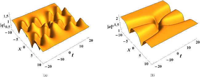
Both the asymptotic expressions ${q}_{{\rm{I}}}^{\pm }$ and ${q}_{{\rm{II}}}^{\pm }$ are the combined dark-bright solitons with the logarithmic center trajectories ${\eta }_{{\rm{I}}}^{\pm }=0$ and ${\eta }_{{\rm{II}}}^{\pm }=0$, respectively. Similar to the conventional soliton solutions with simple poles [49], each asymptotic soliton here exhibits the beating behavior during its evolution over time. However, the difference lies in that such beating behavior is not strictly periodic since the velocities of two solitons change with t at the rate O(t-1). Therefore, equations (4.6a) and (4.6b) can be referred to as the quasi-periodic beating solitons. In addition, given that q(x, t) and q(-x, t) are two components of system (1.1), their superposed intensity |u(x, t)|2 := |q(x, t)|2 + |q(-x, t)|2 shows an elastic interaction between two conserved solitons, i.e. two logarithmically curved dark solitons (see figure 1(b)).
Figure 1. (a) An interaction between two quasi-periodic beating solitons with ${z}_{2,1}=\sqrt{6}{\rm{i}}$, q+ = 1, ${d}_{2,1}=\frac{3}{4}$ and ${l}_{2,1}=-\frac{{\rm{i}}}{8}$. (b) An interaction between two logarithmically curved dark solitons for the superposed intensity |q(x, t)|2 + |q( - x, t)|2.
(ii) n2 = n3 = 0 and n1 = n4 = 1. In this case, one pair of simple poles$\{{\xi }_{1,1},{\xi }_{1,1}^{* }\}$ lies on the circle $\Gamma$, and the other pair of double poles $\{{z}_{2,1},{\hat{z}}_{2,1}\}$ is symmetric about the circle $\Gamma$. Then, we take ${\xi }_{1,1}={\rm{i}}\sqrt{2}{q}_{0}$ and ${z}_{2,1}={\rm{i}}\sqrt{2}\kappa {q}_{0}$ with κ > 1. Based on the constraints (3.14), (3.15) and the constraint of c1,1 described in lemma 3.1 of [49], the norming constants should satisfy the following conditions:
$\begin{eqnarray}\begin{array}{l}{c}_{1,1}=1,| {d}_{2,1}{| }^{2}=\displaystyle \frac{(\kappa +1){\kappa }^{2}{(\kappa -1)}^{3}}{2{({\kappa }^{2}+1)}^{3}},\\ 2\mathrm{Re}({l}_{2,1}{{\rm{e}}}^{{\rm{i}}\mathrm{Arg}({d}_{2,1})})=-\displaystyle \frac{({\kappa }^{2}+2\kappa -1)\sqrt{{\kappa }^{2}-1}}{{({\kappa }^{2}+1)}^{\tfrac{5}{2}}{q}_{0}}.\end{array}\end{eqnarray}$
At the same time, one should notice the following relations:
$\begin{eqnarray}\begin{array}{l}{\theta }_{2}({z}_{2,1})-{\theta }_{1}({z}_{2,1})={\theta }_{1}({\hat{z}}_{2,1})\\ \quad +\,{\theta }_{2}({\hat{z}}_{2,1})=-\frac{\sqrt{2}{q}_{0}}{\kappa }x+\frac{2{\rm{i}}{q}_{0}^{2}}{{\kappa }^{2}}t,\end{array}\end{eqnarray}$
$\begin{eqnarray}{\theta }_{2}({\xi }_{1,1}^{* })=-{\theta }_{1}({\xi }_{1,1})=-2\sqrt{2}{q}_{0}x.\end{eqnarray}$
Then, assuming that $t{{\rm{e}}}^{\mp \frac{\sqrt{2}{q}_{0}}{\kappa }x}=O(1)$, $t{{\rm{e}}}^{\pm \frac{\sqrt{2}{q}_{0}}{\kappa }x}=O(1)$ and x = O(1), respectively, we can use the improved asymptotic analysis method to obtain three non-singular asymptotic solitons as t → ±:
$\begin{eqnarray}\begin{array}{l}{q}_{{\rm{I}}}^{\pm }={q}_{+}\tanh ({\eta }_{{\rm{I}}}^{\pm })\\ \quad \mp \,\frac{{\rm{i}}\sqrt{2}{q}_{+}^{* }(\kappa +1){(\kappa -1)}^{2}}{2{({\kappa }^{2}+1)}^{\frac{3}{2}}{d}_{2,1}}{\rm{{\rm{sech}} }}({\eta }_{{\rm{I}}}^{\pm }){{\rm{e}}}^{\frac{2{\rm{i}}{q}_{0}^{2}}{{\kappa }^{2}}t},\end{array}\end{eqnarray}$
$\begin{eqnarray}\begin{array}{l}{q}_{{\rm{II}}}^{\pm }={q}_{+}\tanh ({\eta }_{{\rm{II}}}^{\pm })\\ \quad \pm \,\frac{{\rm{i}}\sqrt{2}{q}_{-}^{* }(\kappa +1){(\kappa -1)}^{2}}{2{({\kappa }^{2}+1)}^{\frac{3}{2}}{d}_{2,1}}{\rm{{\rm{sech}} }}({\eta }_{{\rm{II}}}^{\pm }){{\rm{e}}}^{\frac{2{\rm{i}}{q}_{0}^{2}}{{\kappa }^{2}}t},\end{array}\end{eqnarray}$
$\begin{eqnarray}{q}_{{\rm{III}}}^{\pm }=-{q}_{+}\tanh (\sqrt{2}{q}_{0}x),\end{eqnarray}$
where
$\begin{eqnarray*}\begin{array}{rcl}{\eta }_{{\rm{I}}}^{\pm } & = & \frac{\sqrt{2}{q}_{0}}{\kappa }x\mp \mathrm{ln}(| t| )\pm \frac{1}{2}\mathrm{ln}\left(\frac{{\kappa }^{4}({\kappa }^{2}+1)}{64{(\kappa +1)}^{2}{q}_{0}^{4}}\right),\\ {\eta }_{{\rm{II}}}^{\pm } & = & \frac{\sqrt{2}{q}_{0}}{\kappa }x\pm \mathrm{ln}(| t| )\mp \frac{1}{2}\mathrm{ln}\left(\frac{{\kappa }^{4}({\kappa }^{2}+1)}{64{(\kappa +1)}^{2}{q}_{0}^{4}}\right).\end{array}\end{eqnarray*}$
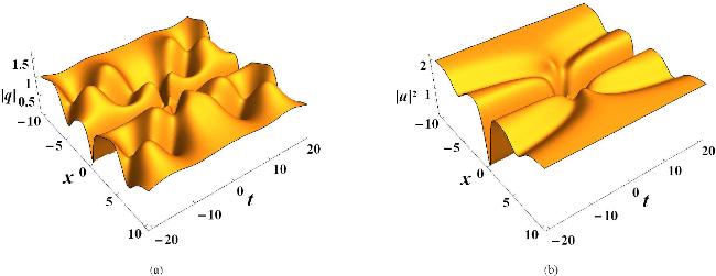
It can be seen that ${q}_{{\rm{I}}}^{\pm }$ and ${q}_{{\rm{II}}}^{\pm }$ are two logarithmically curved beating solitons, which are both quasi-periodic in t and exhibit the phase shift varying logarithmically with t; whereas ${q}_{{\rm{III}}}^{\pm }$ is a static dark soliton which experiences no phase shift. As shown in figures 2(a) and (b), this solution describes an interaction among two propagating quasi-periodic beating solitons and one static dark soliton, which correspond to three dark solitons in the superposed intensity |u|2.
Figure 2. (a) An interaction among two quasi-periodic beating solitons and one static dark soliton with ${\xi }_{2,1}=\sqrt{2}{\rm{i}}$, ${z}_{2,1}=2\sqrt{2}{\rm{i}}$, q+ = 1, c1,1 = 1, ${d}_{2,1}=\frac{\sqrt{30}}{25}$ and ${l}_{2,1}=-\frac{21}{250}{\rm{i}}$. (b) An interaction among two propagating logarithmically curved dark solitons and one static dark soliton for the superposed intensity |q(x, t)|2 + |q( - x, t)|2.
(iii) n1 = n3 = 0 and n2 = n4 = 1. In this case, there are one pair of simple poles $\{{z}_{1,1},{\hat{z}}_{1,1}^{* }\}$ and one pair of double poles $\{{z}_{2,1},{\hat{z}}_{2,1}^{* }\}$, which are symmetrically distributed with respect to the circle $\Gamma$. Then, we define that ${z}_{1,1}={\rm{i}}{\kappa }_{1}\sqrt{2}{q}_{0}$, ${z}_{2,1}={\rm{i}}{\kappa }_{2}\sqrt{2}{q}_{0}$ with κ1, κ2 > 1. By virtue of the constraints (3.14) and (3.15), the norming constants should obey that
$\begin{eqnarray}\begin{array}{l}| {d}_{1,1}{| }^{2}=\displaystyle \frac{{\kappa }_{1}^{^{\prime} }{\kappa }_{1}^{2}{({\kappa }_{1}{\kappa }_{2}-1)}^{2}}{2({\kappa }_{1}^{2}+1){({\kappa }_{1}{\kappa }_{2}+1)}^{2}},\\ | {d}_{2,1}{| }^{2}=\displaystyle \frac{{\kappa }_{2}^{^{\prime} }{\kappa }_{2}^{2}{({\kappa }_{1}{\kappa }_{2}-1)}^{2}}{2({\kappa }_{2}^{2}+1){({\kappa }_{1}{\kappa }_{2}+1)}^{2}},\end{array}\end{eqnarray}$
$\begin{eqnarray}\begin{array}{l}2{\rm{Re}}({l}_{2,1}{{\rm{e}}}^{{\rm{i}}{\rm{Arg}}({d}_{2,1})})\\ \quad =\,\frac{{\kappa }_{1}{\kappa }_{2}^{5}+3{\kappa }_{1}^{2}{\kappa }_{2}^{4}-{\kappa }_{1}^{2}{\kappa }_{2}^{2}-3{\kappa }_{2}^{2}-{\kappa }_{1}{\kappa }_{2}+1}{{({\kappa }_{1}{\kappa }_{2}-1)}^{\frac{1}{2}}{({\kappa }_{1}{\kappa }_{2}+1)}^{\frac{3}{2}}{({\kappa }_{2}^{2}+1)}^{\frac{5}{2}}{q}_{0}},\end{array}\end{eqnarray}$
where ${\kappa }_{1}^{{\prime} }=\frac{{\kappa }_{1}^{2}-1}{{\kappa }_{1}^{2}+1}$ and ${\kappa }_{2}^{{\prime} }=\frac{{\kappa }_{2}^{2}-1}{{\kappa }_{2}^{2}+1}$. Based on the following relations:
$\begin{eqnarray}\begin{array}{l}{\theta }_{2}({z}_{1,1})-{\theta }_{1}({z}_{1,1})={\theta }_{1}({\hat{z}}_{1,1})\\ \quad +\,{\theta }_{2}({\hat{z}}_{1,1})=-\frac{\sqrt{2}{q}_{0}}{{\kappa }_{1}}x+\frac{2{\rm{i}}{q}_{0}^{2}}{{\kappa }_{1}^{2}}t,\end{array}\end{eqnarray}$
$\begin{eqnarray}\begin{array}{l}{\theta }_{2}({z}_{2,1})-{\theta }_{1}({z}_{2,1})={\theta }_{1}({\hat{z}}_{2,1})\\ \quad +\,{\theta }_{2}({\hat{z}}_{2,1})=-\frac{\sqrt{2}{q}_{0}}{{\kappa }_{2}}x+\frac{2{\rm{i}}{q}_{0}^{2}}{{\kappa }_{2}^{2}}t,\end{array}\end{eqnarray}$
we assume that $t{{\rm{e}}}^{\mp \frac{\sqrt{2}{q}_{0}x}{{\kappa }_{2}}}=O(1)$, $t{{\rm{e}}}^{\pm \frac{\sqrt{2}{q}_{0}x}{{\kappa }_{2}}}=O(1)$ and x = O(1) as t → ± , and then obtain three non-singular asymptotic solitons:
$\begin{eqnarray}\begin{array}{l}{q}_{{\rm{I}}}^{\pm }={q}_{+}\tanh ({\eta }_{{\rm{I}}}^{\pm })\pm \frac{{\rm{i}}\sqrt{2}{q}_{+}^{* }{({\kappa }_{2}^{{\prime} })}^{\frac{3}{2}}}{2{d}_{2,1}}\frac{{\kappa }_{1}-{\kappa }_{2}}{| {\kappa }_{1}-{\kappa }_{2}| }\\ \quad \times \,{\left(\frac{{\kappa }_{1}{\kappa }_{2}-1}{{\kappa }_{1}{\kappa }_{2}+1}\right)}^{\frac{1}{2}}{\rm{{\rm{sech}} }}({\eta }_{{\rm{I}}}^{\pm }){{\rm{e}}}^{\frac{2{\rm{i}}{q}_{0}^{2}}{{\kappa }_{2}^{2}}t},\end{array}\end{eqnarray}$
$\begin{eqnarray}\begin{array}{l}{q}_{{\rm{II}}}^{\pm }={q}_{+}\tanh ({\eta }_{{\rm{II}}}^{\pm })\mp \frac{{\rm{i}}\sqrt{2}{q}_{-}^{* }{({\kappa }_{2}^{{\prime} })}^{\frac{3}{2}}}{2{d}_{2,1}}\frac{{\kappa }_{1}-{\kappa }_{2}}{| {\kappa }_{1}-{\kappa }_{2}| }\\ \quad \times \,{\left(\frac{{\kappa }_{1}{\kappa }_{2}-1}{{\kappa }_{1}{\kappa }_{2}+1}\right)}^{\frac{1}{2}}{\rm{{\rm{sech}} }}({\eta }_{{\rm{II}}}^{\pm }){{\rm{e}}}^{\frac{2{\rm{i}}{q}_{0}^{2}}{{\kappa }_{2}^{2}}t},\end{array}\end{eqnarray}$
$\begin{eqnarray}\begin{array}{l}{q}_{{\rm{III}}}^{\pm }=-{q}_{+}\tanh \left(\frac{\sqrt{2}{q}_{0}}{{\kappa }_{1}}x\right)-\frac{\sqrt{2}{q}_{+}^{* }{\kappa }_{1}^{{\prime} }}{2{d}_{1,1}}\\ \quad \times \,\frac{{\kappa }_{1}{\kappa }_{2}-1}{{\kappa }_{1}{\kappa }_{2}+1}{\rm{{\rm{sech}} }}\left(\frac{\sqrt{2}{q}_{0}}{{\kappa }_{1}}x\right){{\rm{e}}}^{\frac{2{\rm{i}}{q}_{0}^{2}}{{\kappa }_{1}^{2}}t},\end{array}\end{eqnarray}$
where
$\begin{eqnarray*}\begin{array}{l}{\eta }_{{\rm{I}}}^{\pm }=\frac{\sqrt{2}{q}_{0}}{{\kappa }_{2}}x\mp \mathrm{ln}(| t| )\\ \quad \pm \frac{1}{2}\mathrm{ln}\left(\frac{{\kappa }_{2}^{4}({\kappa }_{1}{\kappa }_{2}+1){({\kappa }_{1}-{\kappa }_{2})}^{2}}{64{q}_{0}^{4}{\kappa }_{2}^{{\prime} }({\kappa }_{1}{\kappa }_{2}-1){({\kappa }_{1}+{\kappa }_{2})}^{2}}\right),\end{array}\end{eqnarray*}$
$\begin{eqnarray*}\begin{array}{l}{\eta }_{{\rm{II}}}^{\pm }=\frac{\sqrt{2}{q}_{0}}{{\kappa }_{2}}x\pm \mathrm{ln}(| t| )\\ \quad \mp \,\frac{1}{2}\mathrm{ln}\left(\frac{{\kappa }_{2}^{4}({\kappa }_{1}{\kappa }_{2}+1){({\kappa }_{1}-{\kappa }_{2})}^{2}}{64{q}_{0}^{4}{\kappa }_{2}^{{\prime} }({\kappa }_{1}{\kappa }_{2}-1){({\kappa }_{1}+{\kappa }_{2})}^{2}}\right).\end{array}\end{eqnarray*}$
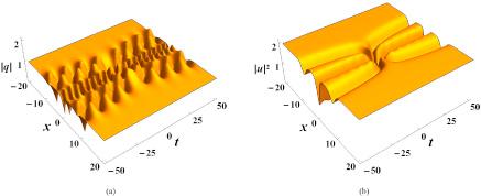
Obviously, both ${q}_{{\rm{I}}}^{\pm }$ and ${q}_{{\rm{II}}}^{\pm }$ are quasi-periodic beating solitons with logarithmically curved center trajectories ${\eta }_{{\rm{I}}}^{\pm }=0$ and ${\eta }_{{\rm{II}}}^{\pm }=0$, respectively, and they have the same t-period $\frac{\pi {\kappa }_{2}^{2}}{{q}_{0}^{2}}$, while ${q}_{{\rm{III}}}^{\pm }$ is the static beating soliton with the t-period $\frac{\pi {\kappa }_{1}^{2}}{{q}_{0}^{2}}$. Again, the phase shifts of ${q}_{{\rm{I}}}^{\pm }$ and ${q}_{{\rm{II}}}^{\pm }$ exhibit the logarithmic dependence of t, but there is no phase shift for ${q}_{{\rm{III}}}^{\pm }$. Thus, this solution displays an interaction among two propagating logarithmically curved quasi-periodic beating solitons and one static beating soliton, as shown in figure 3(a). Meanwhile, the corresponding superposed intensity |u|2 shows an interaction among three dark solitons (see figure 3(b)).
Figure 3. (a) An interaction between two quasi-periodic beating solitons and one static beating soliton with ${z}_{1,1}=\frac{5\sqrt{2}}{4}{\rm{i}}$, ${z}_{2,1}=2\sqrt{2}{\rm{i}}$, q+ = 1, ${d}_{1,1}=\frac{45\sqrt{2}}{574}$, ${d}_{2,1}=\frac{3}{5}\sqrt{\frac{3}{70}}$ and ${l}_{2,1}=-\frac{127}{350}\sqrt{\frac{3}{35}}{\rm{i}}$. (b) An interaction among two propagating logarithmically curved dark solitons and one static dark soliton for the superposed intensity |q(x, t)|2 + |q( - x, t)|2.

5. Conclusion

Equation (1.2) is a physically significant nonlocal NLS equation since it can be derived from the parity-symmetric reduction of the Manakov system. In this work, we have considered that the reciprocals of scattering coefficients have both the simple and double poles, and extended the IST theory for the defocusing equation (1.2) under NZBCs. By analyzing the behavior of the Jost eigenfunction and the auxiliary Jost eigenfunction at double poles, we have regularized the RHP and obtained the extended trace formulas and reconstruction formulas. Meanwhile, based on the symmetries of eigenfunctions and their derivatives, we have derived the complex constraint relations between norming constants.
In the reflectionless case, we have presented the double-pole soliton solutions with NZBCs. Also, we have analyzed the solution dynamical properties for three cases with one double pole by studying the discrete eigenvalue distribution and asymptotic analysis of the solutions. The obtained asymptotic solitons indicate that a double pole off the circle $\Gamma$ can lead to two quasi-periodic beating solitons with logarithmically curved central trajectories. Moreover, their superposed intensity can form a pair of logarithmically curved dark solitons. Considering the coexistence of simple and double poles, one can also observe the interactions between the logarithmically curved beating solitons and either the conventional dark soliton or beating soliton. It should be noted that the number of pure imaginary simple poles must be odd for θ+ - θ- = π (q+ = - q-) and even for θ+ - θ- = 0 (q+ = q-), but there is no such restriction on the double poles. Continually, we can establish the IST theory of equation (1.2) under NZBCs with the presence of multiple poles, and obtain higher-order multi-pole soliton solutions. Similarly, a multiple pole off the circle $\Gamma$ can generate multiple quasi-periodic beating solitons, most of which have logarithmical center trajectories [61, 62]. Meanwhile, the solutions can exhibit a rich variety of soliton interactions; for example, one may observe the interaction among two logarithmically curved beating solitons and a static one when a triple pole lies on the imaginary axis but off the circle $\Gamma$.

This work was supported by the Beijing Natural Science Foundations (Grant Nos. 1232022 and 1252016), the National Natural Science Foundations of China (Grant Nos. 12475003 and 11705284), and the Hebei Province Natural Science Foundation (Grant No. A2025502019).

[1]
Manakov S V 1974 On the theory of two-dimensional stationary self-focusing of electromagnetic waves Sov. Phys. JETP 38 248 253

[2]
Hoefer M A, Chang J J, Hamner C, Engels P 2011 Dark-dark solitons and modulational instability in miscible two-component Bose-Einstein condensates Phys. Rev. A 84 041605

DOI

[3]
Kamchatnov A M, Sokolov V V 2015 Nonlinear waves in two-component Bose-Einstein condensates: Manakov system and Kowalevski equations Phys. Rev. A 91 043621

DOI

[4]
Menyuk C R 1987 Stability of solitons in birefringent optical fibers: I. Equal propagation amplitudes Opt. Lett. 12 614 616

DOI

[5]
Evangelides S G, Mollenauer L F, Gordon J P, Bergano N S 1992 Polarization multiplexing with solitons J. Lightwave Technol. 10 28 35

DOI

[6]
Wai P K A, Menyuk C R 1996 Polarization mode dispersion, decorrelation, and diffusion in optical fibers with randomly varying birefringence J. Lightwave Technol. 14 148 157

DOI

[7]
Frisquet B, Kibler B, Fatome J, Morin P, Baronio F, Conforti M, Millot G, Wabnitz S 2015 Polarization modulation instability in a Manakov fiber system Phys. Rev. A 92 053854

DOI

[8]
Ankiewicz A, Królikowski W, Akhmediev N N 1999 Partially coherent solitons of variable shape in a slow Kerr-like medium: exact solutions Phys. Rev. E 59 6079 6087

DOI

[9]
Onorato M, Osborne A R, Serio M 2006 Modulational instability in crossing sea states: a possible mechanism for the formation of freak waves Phys. Rev. Lett. 96 014503

DOI

[10]
Docksey R G, Elgin J N 2000 Closure of the Manakov system SIAM J. Math. Anal. 32 54 79

DOI

[11]
Wang D S, Zhang D J, Yang J K 2010 Integrable properties of the general coupled nonlinear Schrödinger equations J. Math. Phys. 51 023510

DOI

[12]
Kodama Y, Mikhailov A V 2001 Symmetry and perturbation of the vector nonlinear Schrödinger equation Physica D 152-153 171 177

DOI

[13]
Sahadevan R, Tamizhmani K, Lakshmanan M 1986 Painlevé analysis and integrability of coupled non-linear Schrödinger equations J. Phys. A: Math. Gen. 19 1783 1791

DOI

[14]
Porsezian K, Nakkeeran K J P 1997 Optical solitons in birefringent fibre-Bäcklund transformation approach Pure Appl. Opt. 6 L7

DOI

[15]
C. Wright O, Gregory Forest M 2000 On the Bäcklund-gauge transformation and homoclinic orbits of a coupled nonlinear Schrödinger system Physica D 141 104 116

DOI

[16]
Radhakrishnan R, Lakshmanan M 1995 Bright and dark soliton solutions to coupled nonlinear Schrödinger equations J. Phys. A: Math. Gen. 28 2683 2692

DOI

[17]
Stalin S, Ramakrishnan R, Senthilvelan M, Lakshmanan M 2019 Nondegenerate solitons in Manakov system Phys. Rev. Lett. 122 043901

DOI

[18]
Xu T, Tian B 2010 Bright N-soliton solutions in terms of the triple Wronskian for the coupled nonlinear Schrödinger equations in optical fibers J. Phys. A: Math. Theor. 43 245205

DOI

[19]
Xu T, Tian B 2010 An extension of the Wronskian technique for the multicomponent Wronskian solution to the vector nonlinear Schrödinger equation J. Math. Phys. 51 033504

DOI

[20]
Xu T, Tian B, Xue Y S, Qi F H 2010 Direct analysis of the bright-soliton collisions in the focusing vector nonlinear Schrödinger equation Europhys. Lett. 92 50002

DOI

[21]
Radhakrishnan R, Lakshmanan M, Hietarinta J 1997 Inelastic collision and switching of coupled bright solitons in optical fibers Phys. Rev. E 56 2213 2216

DOI

[22]
Kanna T, Lakshmanan M 2001 Exact soliton solutions, shape changing collisions, and partially coherent solitons in coupled nonlinear Schrödinger equations Phys. Rev. Lett. 86 5043 5046

DOI

[23]
Kanna T, Lakshmanan M 2003 Exact soliton solutions of coupled nonlinear Schrödinger equations: shape-changing collisions, logic gates, and partially coherent solitons Phys. Rev. E 67 046617

DOI

[24]
Gao X, Meng L Z, Zhao L C 2025 Dark-bright solitons with positive mass in Manakov cases with repulsive interactions Phys. Rev. E 111 054209

DOI

[25]
Chen S C, Liu C, Yao X, Zhao L C, Akhmediev N 2021 Extreme spectral asymmetry of Akhmediev breathers and Fermi-Pasta-Ulam recurrence in a Manakov system Phys. Rev. E 104 024215

DOI

[26]
Baronio F, Degasperis A, Conforti M, Wabnitz S 2012 Solutions of the vector nonlinear Schrödinger equations: evidence for deterministic rogue waves Phys. Rev. Lett. 109 044102

DOI

[27]
Guo B L, Ling L M 2011 Rogue wave, breathers and bright-dark-rogue solution for the coupled Schrödinger equations Chin. Phys. Lett. 28 110202

DOI

[28]
Xu L, Wang D S, Wen X Y, Jiang Y L 2020 Exotic localized vector waves in a two-component nonlinear wave system J. Nonl. Sci. 30 537 564

DOI

[29]
Vijayajayanthi M, Kanna T, Lakshmanan M 2023 Simulation of universal optical logic gates under energy sharing collisions of Manakov solitons and fulfillment of practical optical logic criteria Phys. Rev. E 108 054213

DOI

[30]
Anastassiou C, Segev M, Steiglitz K, Giordmaine J, Mitchell M, Shih M F, Lan S, John M 1999 Energy-exchange interactions between colliding vector solitons Phys. Rev. Lett. 83 2332 2335

DOI

[31]
Rand D, Glesk I, Brès C S, Nolan D A, Chen X, Koh J, Fleischer J W, Steiglitz K, Prucnal P R 2007 Observation of temporal vector soliton propagation and collision in birefringent fiber Phys. Rev. Lett. 98 053902

DOI

[32]
Jakubowski M H, Steiglitz K, Squier R 1998 State transformations of colliding optical solitons and possible application to computation in bulk media Phys. Rev. E 58 6752 6758

DOI

[33]
Steiglitz K 2000 Time-gated Manakov spatial solitons are computationally universal Phys. Rev. E 63 016608

DOI

[34]
Si Z Z, Wang Y Y, Dai C Q 2024 Switching, explosion, and chaos of multi-wavelength soliton states in ultrafast fiber lasers Sci. China Phys. Mech. Astron. 67 274211

DOI

[35]
Si Z Z, Ju Z T, Ren L F, Wang X P, Malomed B A, Dai C Q 2025 Polarization-induced buildup and switching mechanisms for soliton molecules composed of noise-like-pulse transition states Laser Photonics Rev. 19 2401019

DOI

[36]
Ablowitz M J, Musslimani Z H 2013 Integrable nonlocal nonlinear Schrödinger equation Phys. Rev. Lett. 110 064105

DOI

[37]
Ablowitz M J, Prinari B, Trubatch A D 2004 Discrete and Continuous Nonlinear Schrödinger Systems Cambridge University Press

[38]
Biondini G, Kraus D 2015 Inverse scattering transform for the defocusing Manakov system with nonzero boundary conditions SIAM J. Math. Anal. 47 706 757

DOI

[39]
Prinari B, Ablowitz M J, Biondini G 2006 Inverse scattering transform for the vector nonlinear Schrödinger equation with non-vanishing boundary conditions J. Math. Phys. 47 063508

DOI

[40]
Dean G, Klotz T, Prinari B, Vitale F 2013 Dark-dark and dark-bright soliton interactions in the two-component defocusing nonlinear Schrödinger equation Appl. Anal. 92 379 397

DOI

[41]
Kraus D, Biondini G, Kovačič G 2015 The focusing Manakov system with nonzero boundary conditions Nonlinearity 28 3101 3151

DOI

[42]
Abeya A, Biondini G, Prinari B 2022 Inverse scattering transform for the defocusing Manakov system with non-parallel boundary conditions at infinity East Asian J. Appl. Math. 12 715 760

DOI

[43]
Abeya A, Biondini G, Prinari B 2022 Manakov system with parity symmetry on nonzero background and associated boundary value problems J. Phys. A-Math. Theor. 25 254001

DOI

[44]
Yang J K 2018 Physically significant nonlocal nonlinear Schrödinger equation and its soliton solutions Phys. Rev. E 98 042202

DOI

[45]
Wu J P 2023 A novel Riemann-Hilbert approach via t-part spectral analysis for a physically significant nonlocal integrable nonlinear Schrödinger equation Nonlinearity 36 2021 2037

DOI

[46]
Wu J P 2025 A novel Riemann-Hilbert formulation-based reduction method to an integrable reverse-space nonlocal Manakov equation and its applications Chaos Soliton. Fract. 192 115997

DOI

[47]
Chen J C, Yan Q X, Zhang H 2020 Multiple bright soliton solutions of a reverse-space nonlocal nonlinear Schrödinger equation Appl. Math. Lett. 106 106375

DOI

[48]
Wang X, He J S 2024 Rogue waves in a reverse space nonlocal nonlinear Schrödinger equation Physica D 469 134313

DOI

[49]
Xu C X, Xu T, Li M 2025 Inverse scattering transform for the defocusing nonlinear Schrödinger equation with local and nonlocal nonlinearities under non-zero boundary conditions Lett. Math. Phys. 115 105

DOI

[50]
Xu C, Xu T, Li M, Huang Y H 2025 Inverse scattering transform for the focusing PT-symmetric nonlinear Schrödinger equation with nonzero boundary conditions: higher-order poles and multi-soliton solutions Physica D 472 134466

DOI

[51]
Zakharov V E, Shabat A B 1972 Exact theory of two-dimensional self-focusing and one-dimensional selfmodulation of waves in nonlinear media Sov. Phys. JETP 34 62 69

[52]
Wadati M, Ohkuma K 1982 Multiple-pole solutions of the modified Korteweg-de Vries equation J. Phys. Soc. Jpn. 51 2029 2035

DOI

[53]
Olmedilla E 1987 Multiple pole solutions of the nonlinear Schrödinger equation Physica D 25 330 346

DOI

[54]
Shchesnovich V, Yang J 2003 General soliton matrices in the Riemann-Hilbert problem for integrable nonlinear equations J. Math. Phys. 44 4604 4639

DOI

[55]
Biondini G, Kovačič G 2014 Inverse scattering transform for the focusing nonlinear Schrödinger equation with non-zero boundary conditions and double-poles J. Math. Phys. 55 031506

DOI

[56]
Yang J J, Tian S F, Li Z Q 2022 Riemann-Hilbert problem for the focusing nonlinear Schrödinger equation with multiple high-order poles under nonzero boundary conditions Physica D 432 133162

DOI

[57]
Bilman D, Buckingham R, Wang D S 2021 Far-field asymptotics for multiple-pole solitons in the large-order limit J. Differ. Equ. 297 320 369

DOI

[58]
Xu T, Lan S, Li M, Li L L, Zhang G W 2019 Mixed soliton solutions of the defocusing nonlocal nonlinear Schrödinger equation Physica D 390 47 61

DOI

[59]
Li M, Zhang X F, Xu T, Li L L 2020 Asymptotic analysis and soliton interactions of the multi-pole solutions in the Hirota equation J. Phys. Soc. Jpn. 85 124001

DOI

[60]
Xu T, Li L L, Li M, Li C X, Zhang X F 2021 Rational solutions of the defocusing non-local nonlinear Schrödinger equation: asymptotic analysis and soliton interactions Proc. R. Soc. A 477 20210512

DOI

[61]
Li M, Zhang X F, Xu T, Li L L 2020 Asymptotic analysis and soliton interactions of the multi-pole solutions in the Hirota equation J. Phys. Soc. Jpn. 89 054004

DOI

[62]
Zhang S S, Xu T, Li M, Zhang X F 2022 Higher-order algebraic soliton solutions of the Gerdjikov-Ivanov equation: asymptotic analysis and emergence of rogue waves Physica D 432 133128

DOI

Outlines

/