


1. Introduction
In conventional quantum mechanics, the Hamiltonian is required to be Hermitian to ensure real energy eigenvalues and probability conservation. However, in 1998, Bender and Boettcher proposed that non-Hermitian Hamiltonians with parity-time (PT) symmetric constraint can also yield real energy spectra [1]. This theoretical breakthrough challenges the strict requirement of Hermiticity, demonstrating that non-Hermitian systems can maintain physical stability when the combined space-time symmetry is preserved. In recent years, PT-symmetric systems have been experimentally realized, for instance, through the design of optical waveguides with balanced gain/loss distributions [2], offering novel platforms for manipulating wave propagation, achieving unidirectional invisibility, and exploiting exceptional point sensing [3]. In the field of nonlinear wave dynamics, the nonlinear Schrödinger equation (NLSE) serves as a fundamental model for describing phenomena such as optical solitons and Bose-Einstein condensation [4]. When a PT-symmetric potential of the form $V(x)={V}_{{\rm{re}}}(x)+{\rm{i}}{V}_{{\rm{im}}}(x)$ is introduced, the system must satisfy the following symmetry conditions [5]
$\begin{eqnarray}{V}_{{\rm{re}}}(-x)={V}_{{\rm{re}}}(x),\quad {V}_{{\rm{im}}}(-x)=-{V}_{{\rm{im}}}(x).\end{eqnarray}$
This non-Hermitian extension endows the NLSE with new physical significance: the real part ${V}_{{\rm{re}}}$ modulates the refractive index distribution, while the imaginary part ${V}_{{\rm{im}}}$ breaks the constraint of energy conservation through a gain-loss balance mechanism, enabling stable propagation of nonlinear waves in open environments. This substantially broadens the applicability of the NLSE [6]. The resulting exotic phenomena, such as nonreciprocal transmission and nonlinear exceptional points [7], provide a theoretical foundation for the design of nonreciprocal optical devices and ultrasensitive sensors. However, the explicit form of the potential function is typically based on prior assumptions and is difficult to measure directly in experiments [3, 8], presenting a major bottleneck in the design of PT-symmetric devices.In practical applications, usually only partial observational data of the system, such as the evolution trajectory of the wave function, can be obtained, while the potential function itself is not directly observable. Therefore, how to infer the PT-symmetric potential function from limited observational data becomes a key issue. Traditional inversion methods, such as variational methods and least-squares optimization, though effective in low-dimensional linear scenarios [9, 10], often suffer from high computational complexity [11] and poor convergence [12] when dealing with high-dimensional and strongly nonlinear systems. In recent years, physics-informed neural networks (PINNs), as an emerging deep learning method, have provided a new approach for solving such inverse problems. PINNs incorporate physical equations into the loss function to constrain the learning process of neural networks, enabling the networks to not only fit the observational data but also satisfy physical constraints [13]. Zhou et al [14] employed PINNs to jointly solve the forward and inverse problems of the logarithmic NLSE with PT-symmetric harmonic potential, successfully identifying the dispersion coefficient, nonlinear coefficient, and amplitude of the PT-symmetric harmonic potential in the equation. Li et al [15], targeting the NLSE with generalized PT-symmetric Scarf-II potential, systematically investigated both forward and parameter inversion problems using a hybrid framework combining PINNs and data-driven techniques. They successfully inferred the amplitude parameters of the generalized PT-symmetric Scarf-II potential, as well as the coefficients of the dispersion and nonlinear terms. Peng et al [16] proposed a PTS-PINNs method by incorporating PT-symmetry information into the loss function of PINNs, effectively addressing the inverse problem of the NLSE. In addition, some researchers have enhanced the performance of PINNs for both forward and inverse problems by directly improving the network architecture. For example, Qiu et al [17], in solving forward and inverse problems of the 2-coupled mixed derivative NLSE, proposed an innovative framework combining PINNs with generative adversarial networks (GAN), namely the physics-informed GAN with gradient penalty. This method embeds PINNs as the generator in the GAN framework, directly solving the equation and predicting soliton dynamics under physical constraints, while introducing a gradient penalty mechanism to overcome the training instability of traditional GANs. Song et al [18], targeting the inversion of PT-symmetric potential functions in one- and two-dimensional saturable NLSE, proposed a modified PINNs (mPINNs). This method enables direct identification of PT-symmetric potentials, including Scarf-II type and periodic type, from solution data, overcoming the limitation of traditional methods that can only invert potential parameters.
This paper investigates the inverse problem associated with a class of (1 + 1)-dimensional nonlinear PT-symmetric NLSEs. The equations take the form
$\begin{eqnarray}\begin{array}{l}{\rm{i}}{u}_{t}(x,t)+{u}_{xx}(x,t)+\gamma V(x)u(x,t)+F\left(u(x,t)\right)=0,\\ x\in [{x}_{l},{x}_{r}],\quad t\in [0,T].\end{array}\end{eqnarray}$
Here, u(x, t) represents the wave function, $\gamma$ is a known constant, F(u) is the nonlinear term, and V(x) is a complex-valued potential function satisfying PT-symmetry. The aim of this study is to reconstruct the unknown potential function V(x) based on limited observational data ${\{u({x}_{j},{t}_{j})\}}_{j=1}^{N}$, under the assumption that the initial and boundary conditions are known. The main contributions of this paper include:●A novel parallel deep neural network architecture, termed parallel PT-symmetric PINNs (PPTS-PINNs), is proposed for the full-field inversion of the potential function. This architecture employs independent subnetworks to reconstruct different components of the potential, with PT-symmetry constraints directly imposed on the subnetworks to ensure that the reconstructed potential satisfies the symmetry condition (1 ).
●A gradient enhancement strategy [19] is incorporated, enabling the model to maintain high inversion accuracy even under high noise levels.
The structure of this paper is organized as follows: section 2 briefly reviews the methodological foundations of PINNs for solving forward and inverse problems of partial differential equation (PDE). Section 3 details the construction of the data-driven method PPTS-PINNs, which integrates physical constraints and introduces a gradient enhancement strategy to improve model stability and accuracy under noisy conditions. Section 4 presents several representative numerical experiments to evaluate the inversion performance of the proposed method under varying noise levels. Section 5 concludes the paper by summarizing the proposed algorithmic framework, outlining its advantages and current limitations, and discussing possible directions for future improvement and application.
2. Methodological foundations of PINNs for forward and inverse PDE problems
Consider a generalized PDE with known or unknown parameters λ, expressed as
$\begin{eqnarray}{ \mathcal N }[u({\boldsymbol{x}});\,{\boldsymbol{\lambda }}]=0,\quad {\boldsymbol{x}}\in {\rm{\Omega }},\end{eqnarray}$
subject to appropriate conditions on the boundary (or at the initial time) of the domain ${\rm{\Omega }}\subset {{\mathbb{R}}}^{d}$ $\begin{eqnarray}{ \mathcal B }[u({\boldsymbol{x}})]=0,\quad {\boldsymbol{x}}\in \partial {\rm{\Omega }}.\end{eqnarray}$
Here, ${ \mathcal N }$ denotes the differential operator, ${ \mathcal B }$ represents the boundary or initial condition operator, λ refers to the unknown or identifiable parameters in the PDE, and u(x) is the target field to be solved. For spatiotemporal problems, time t is treated as a special component of x, and ${ \mathcal B }$ includes both the initial condition at t = 0 and the spatial boundary conditions.2.1. Solving forward PDE problems using PINNs
In forward problems, the parameters λ are known, and the objective is to obtain a numerical solution u(x) that satisfies both equations (3 ) and (4 ).
To begin, a neural network uθ(x) is constructed to approximate u(x), where θ denotes the parameters of the network. This network acts as a surrogate model for the solution of the PDE.
Then, a loss function is formulated based on the residuals of the PDE and boundary conditions. A set of collocation points ${{ \mathcal T }}_{f}$ is selected in the domain Ω, and a set of boundary points ${{ \mathcal T }}_{b}$ is selected on the boundary ∂Ω. The loss function is defined as
$\begin{eqnarray}{ \mathcal L }({\boldsymbol{\theta }})={w}_{f}\,{{ \mathcal L }}_{f}({\boldsymbol{\theta }})+{w}_{b}\,{{ \mathcal L }}_{b}({\boldsymbol{\theta }}),\end{eqnarray}$
where $\begin{eqnarray*}\begin{array}{rcl}{{ \mathcal L }}_{f}({\boldsymbol{\theta }}) & = & \frac{1}{| {{ \mathcal T }}_{f}| }\displaystyle \sum _{{{\boldsymbol{x}}}_{f}\in {{ \mathcal T }}_{f}}{\parallel { \mathcal N }[{u}_{{\boldsymbol{\theta }}}({{\boldsymbol{x}}}_{f});\,{\boldsymbol{\lambda }}]\parallel }^{2},\\ {{ \mathcal L }}_{b}({\boldsymbol{\theta }}) & = & \frac{1}{| {{ \mathcal T }}_{b}| }\displaystyle \sum _{{{\boldsymbol{x}}}_{b}\in {{ \mathcal T }}_{b}}{\parallel { \mathcal B }[{u}_{{\boldsymbol{\theta }}}({{\boldsymbol{x}}}_{b})]\parallel }^{2}.\end{array}\end{eqnarray*}$
Here, wf and wb are user-defined weights for the respective loss terms.Finally, the loss function ${ \mathcal L }({\boldsymbol{\theta }})$ is minimized using an optimization algorithm to obtain the optimal parameters
$\begin{eqnarray*}{{\boldsymbol{\theta }}}^{* }=\arg \mathop{\min }\limits_{{\boldsymbol{\theta }}}\,{ \mathcal L }({\boldsymbol{\theta }}),\end{eqnarray*}$
thereby constructing an approximate solution ${u}_{{{\boldsymbol{\theta }}}^{* }}({\boldsymbol{x}})$ that satisfies the PDE and boundary conditions.2.2. Solving inverse PDE problems using PINNs
In inverse problems, certain parameters λ in the PDE are unknown and need to be inferred from observational data. In addition to satisfying (3 ) and (4 ), additional measurement data are available at a set of sampling points ${{ \mathcal T }}_{m}\subset {\rm{\Omega }}$, and satisfy the condition
$\begin{eqnarray*}{ \mathcal M }[{u}_{{\boldsymbol{\theta }}},{{\boldsymbol{x}}}_{m}]=0,\quad {{\boldsymbol{x}}}_{m}\in {{ \mathcal T }}_{m}.\end{eqnarray*}$
To solve such inverse problems, a neural network uθ(x) is first constructed to approximate u(x), and the unknown parameters λ are treated as additional trainable variables alongside the network parameters θ.
A loss function is then constructed by selecting collocation points ${{ \mathcal T }}_{f}$ in the domain, boundary points ${{ \mathcal T }}_{b}$, and observation points ${{ \mathcal T }}_{m}$. The total loss includes residual terms for the PDE and boundary conditions, as well as a data mismatch term. It is defined as
$\begin{eqnarray}{ \mathcal L }({\boldsymbol{\theta }},{\boldsymbol{\lambda }})={w}_{f}\,{{ \mathcal L }}_{f}({\boldsymbol{\theta }},{\boldsymbol{\lambda }})+{w}_{b}\,{{ \mathcal L }}_{b}({\boldsymbol{\theta }},{\boldsymbol{\lambda }})+{w}_{m}\,{{ \mathcal L }}_{m}({\boldsymbol{\theta }},{\boldsymbol{\lambda }}),\end{eqnarray}$
where $\begin{eqnarray*}{{ \mathcal L }}_{m}({\boldsymbol{\theta }},{\boldsymbol{\lambda }})=\frac{1}{| {{ \mathcal T }}_{m}| }\displaystyle \sum _{{{\boldsymbol{x}}}_{m}\in {{ \mathcal T }}_{m}}{\parallel { \mathcal M }[{u}_{{\boldsymbol{\theta }}},{{\boldsymbol{x}}}_{m}]\parallel }^{2}.\end{eqnarray*}$
The term ${{ \mathcal L }}_{m}({\boldsymbol{\theta }},{\boldsymbol{\lambda }})$ quantifies the deviation between the network output and the observational data, and wm is the corresponding loss weight.Finally, both the neural network parameters θ and the unknown physical parameters λ are optimized by minimizing the loss function
$\begin{eqnarray*}({{\boldsymbol{\theta }}}^{* },{{\boldsymbol{\lambda }}}^{* })=\arg \mathop{\min }\limits_{{\boldsymbol{\theta }},{\boldsymbol{\lambda }}}\,{ \mathcal L }({\boldsymbol{\theta }},{\boldsymbol{\lambda }}).\end{eqnarray*}$
This yields the trained network solution ${u}_{{{\boldsymbol{\theta }}}^{* }}({\boldsymbol{x}})$ and the inferred parameters λ*.3. Data-driven methods integrating physical constraints
In this section, we first determine the values of the potential function V(x) at boundary points by constructing auxiliary equations. Subsequently, we present a systematic analysis and explanation of the PPTS-PINNs method, which incorporates a gradient enhancement strategy.
3.1. Inference of V(x) at boundary points
If the boundary and initial conditions of the NLSE (2 ) are known, they can be expressed as 2 ) and (7 ), a system of equations can be constructed at (xl, 0) and (xr, 0)7 ) into the above equations yields
$\begin{eqnarray}\begin{array}{rcl}u({x}_{l},t) & = & {\varphi }_{l}(t)={\varphi }_{{\rm{re}}}^{l}(t)+{\rm{i}}{\varphi }_{{\rm{im}}}^{l}(t),\\ u({x}_{r},t) & = & {\varphi }_{r}(t)={\varphi }_{{\rm{re}}}^{r}(t)+{\rm{i}}{\varphi }_{{\rm{im}}}^{r}(t),\\ u(x,0) & = & \psi (x)={\psi }_{{\rm{re}}}(x)+{\rm{i}}{\psi }_{{\rm{im}}}(x).\end{array}\end{eqnarray}$
By combining equations ( $\begin{eqnarray}\left\{\begin{array}{l}{\rm{i}}{u}_{t}({x}_{l},0)+{u}_{xx}({x}_{l},0)+\gamma V({x}_{l})u({x}_{l},0)+F\left(u({x}_{l},0)\right)=0,\\ {\rm{i}}{u}_{t}({x}_{r},0)+{u}_{xx}({x}_{r},0)+\gamma V({x}_{r})u({x}_{r},0)+F\left(u({x}_{r},0)\right)=0.\end{array}\right.\end{eqnarray}$
Substituting the initial and boundary conditions from ( $\begin{eqnarray}\left\{\begin{array}{l}{\rm{i}}{\left.\frac{\partial {\varphi }_{l}}{\partial t}\right|}_{t=0}+{\psi }_{xx}({x}_{l})+\gamma V({x}_{l}){\varphi }_{l}(0)+F\left({\varphi }_{l}(0)\right)=0,\\ {\rm{i}}{\left.\frac{\partial {\varphi }_{r}}{\partial t}\right|}_{t=0}+{\psi }_{xx}({x}_{r})+\gamma V({x}_{r}){\varphi }_{r}(0)+F\left({\varphi }_{r}(0)\right)=0.\end{array}\right.\end{eqnarray}$
By directly solving (9 ), the values of V(x) at the boundary points xl and xr can be obtained, and denoted as
$\begin{eqnarray*}\begin{array}{rcl}V({x}_{l}) & = & {V}_{{\rm{re}}}^{l}+{\rm{i}}{V}_{{\rm{im}}}^{l},\\ V({x}_{r}) & = & {V}_{{\rm{re}}}^{r}+{\rm{i}}{V}_{{\rm{im}}}^{r}.\end{array}\end{eqnarray*}$
3.2. PPTS-PINNs
To infer the potential function V(x) from limited observational data, we designed a specialized deep learning architecture, referred to as the PPTS-PINNs. As shown in figure 1, the PPTS-PINNs consist of three subnetworks, each implemented using a binary structured neural network (BsNN) [22]. As illustrated in figure 2, the BsNN adopts a binary tree-like connection pattern. Each hidden layer is divided into several 'neuron blocks', with each block connecting only to two blocks in the next layer, thereby progressively reducing the number of connections layer by layer. This design not only lowers the computational complexity but also enhances the network's ability to capture local features of functions. Compared to the traditional feedforward neural network (FNN), the BsNN has significantly fewer parameters when the network depth is large, which helps alleviate overfitting issues.
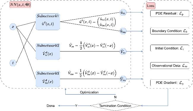
Figure 1. PPTS-PINNs: the left block represents a neural network parameterized by $\Theta$, while the right block denotes the loss function components. |
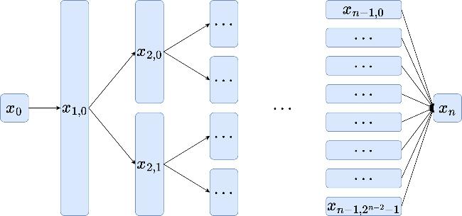
Figure 2. Binary structured neural network. |
The output of the PPTS-PINNs is a real-valued vector. Before detailing the architecture of PPTS-PINNs, we first introduce the following mathematical notations
$\begin{eqnarray*}\begin{array}{rcl}u(x,t) & = & {u}_{{\rm{re}}}(x,t)+{\rm{i}}{u}_{{\rm{im}}}(x,t),\\ V(x) & = & {V}_{{\rm{re}}}(x)+{\rm{i}}{V}_{{\rm{im}}}(x).\end{array}\end{eqnarray*}$
The first subnetwork is denoted as ${\hat{u}}^{\theta }(x,t)$, where θ emphasizes that it is a parameterized function, and it is defined as
$\begin{eqnarray*}{\hat{u}}^{\theta }(x,t)=\left(\begin{array}{c}{\hat{u}}_{{\rm{re}}}(x,t)\\ {\hat{u}}_{{\rm{im}}}(x,t)\end{array}\right).\end{eqnarray*}$
During the training of PT-symmetric PINNs, ${\hat{u}}_{{\rm{re}}}(x,t)$ and ${\hat{u}}_{{\rm{im}}}(x,t)$ are used to approximate ${u}_{{\rm{re}}}(x,t)$ and ${u}_{{\rm{im}}}(x,t)$, respectively. The second and third subnetworks, ${\hat{V}}_{{\rm{re}}}^{\theta }(x)$ and ${\hat{V}}_{{\rm{im}}}^{\theta }(x)$, are used to construct ${\hat{V}}_{{\rm{re}}}(x)$ and ${\hat{V}}_{{\rm{im}}}(x)$ via the following PT-symmetry constraints
$\begin{eqnarray}\begin{array}{rcl}{\hat{V}}_{{\rm{re}}} & = & \frac{1}{2}\left({\hat{V}}_{{\rm{re}}}^{\theta }(x)+{\hat{V}}_{{\rm{re}}}^{\theta }(-x)\right),\\ {\hat{V}}_{{\rm{im}}} & = & \frac{1}{2}\left({\hat{V}}_{{\rm{im}}}^{\theta }(x)-{\hat{V}}_{{\rm{im}}}^{\theta }(-x)\right).\end{array}\end{eqnarray}$
We use ${\hat{V}}_{{\rm{re}}}(x)$ and ${\hat{V}}_{{\rm{im}}}(x)$ to approximate ${V}_{{\rm{re}}}(x)$ and ${V}_{{\rm{im}}}(x)$, and the constraint (10 ) enforces them to satisfy the PT-symmetric condition given in equation (1 ).
Let
$\begin{eqnarray*}\begin{array}{rcl}\hat{u}(x,t) & = & {\hat{u}}_{{\rm{re}}}(x,t)+{\rm{i}}{\hat{u}}_{{\rm{im}}}(x,t),\\ \hat{V}(x) & = & {\hat{V}}_{{\rm{re}}}(x)+{\rm{i}}{\hat{V}}_{{\rm{im}}}(x).\end{array}\end{eqnarray*}$
We use $\hat{u}(x,t)$ and $\hat{V}(x)$ to approximate the complex-valued solution u(x, t) and potential function V(x), respectively. The residual form of the PDE can then be expressed as
$\begin{eqnarray}\begin{array}{rcl}{ \mathcal P }(x,t) & = & { \mathcal D }\left({\hat{u}}_{{\rm{re}}}(x,t),{\hat{u}}_{{\rm{im}}}(x,t),{\hat{V}}_{{\rm{re}}}(x),{\hat{V}}_{{\rm{im}}}(x)\right)\\ & = & {\rm{i}}{\hat{u}}_{t}(x,t)+{\hat{u}}_{xx}(x,t)+\gamma \hat{V}(x)\hat{u}(x,t)+F\left(\hat{u}(x,t)\right)\\ & = & {{ \mathcal P }}_{{\rm{re}}}(x,t)+{\rm{i}}{{ \mathcal P }}_{{\rm{im}}}(x,t).\end{array}\end{eqnarray}$
Let all trainable parameters of PPTS-PINNs be denoted by $\Theta$. We select the interior collocation points ${{ \mathcal T }}_{p}\subset [{x}_{l},{x}_{r}]\times [0,T]$, the left boundary collocation points ${{ \mathcal T }}_{b}^{l}\subset \{{x}_{l}\}\times [0,T]$, the right boundary collocation points ${{ \mathcal T }}_{b}^{r}\subset \{{x}_{r}\}\times [0,T]$, the initial time collocation points ${{ \mathcal T }}_{i}\subset [{x}_{l},{x}_{r}]\times \{0\}$, and the observation points ${{ \mathcal T }}_{m}\subset [{x}_{l},{x}_{r}]\times [0,T]$. The total loss function is defined as follows
$\begin{eqnarray}\begin{array}{rcl}{ \mathcal L }({\boldsymbol{\Theta }}) & = & {{ \mathcal L }}_{p}({\boldsymbol{\Theta }};{{ \mathcal T }}_{p})+{{ \mathcal L }}_{b}({\boldsymbol{\Theta }};{{ \mathcal T }}_{b}^{l},{{ \mathcal T }}_{b}^{r})+{{ \mathcal L }}_{i}({\boldsymbol{\Theta }};{{ \mathcal T }}_{i})\\ & & +{{ \mathcal L }}_{m}({\boldsymbol{\Theta }};{{ \mathcal T }}_{m}).\end{array}\end{eqnarray}$
Specifically,
$\begin{eqnarray}\begin{array}{l}{{ \mathcal L }}_{p}({\boldsymbol{\Theta }};{{ \mathcal T }}_{p})=\displaystyle \frac{1}{\left|{{ \mathcal T }}_{p}\right|}\displaystyle \sum _{({x}_{p},{t}_{p})\in {{ \mathcal T }}_{p}}\left({\left|{{ \mathcal P }}_{\mathrm{re}}({x}_{p},{t}_{p})\right|}^{2}\right.\\ \quad +\,\left.{\left|{{ \mathcal P }}_{\mathrm{im}}({x}_{p},{t}_{p})\right|}^{2}\right),\\ {{ \mathcal L }}_{b}({\boldsymbol{\Theta }};{{ \mathcal T }}_{b}^{l},{{ \mathcal T }}_{b}^{r})=\displaystyle \frac{1}{\left|{{ \mathcal T }}_{b}^{l}\right|}\displaystyle \sum _{({x}_{l},{t}_{b}^{l})\in {{ \mathcal T }}_{b}^{l}}\left({\left|{\hat{u}}_{\mathrm{re}}({x}_{l},{t}_{b}^{l})-{\varphi }_{\mathrm{re}}^{l}({t}_{b}^{l})\right|}^{2}\right.\\ \quad +\,\left.{\left|{\hat{u}}_{\mathrm{im}}({x}_{l},{t}_{b}^{l})-{\varphi }_{\mathrm{im}}^{l}({t}_{b}^{l})\right|}^{2}\right)\\ \quad +\,{\left|{\hat{V}}_{\mathrm{re}}({x}_{l})-{V}_{\mathrm{re}}^{l}\right|}^{2}+{\left|{\hat{V}}_{\mathrm{im}}({x}_{l})-{V}_{\mathrm{im}}^{l}\right|}^{2}\\ \quad +\,\displaystyle \frac{1}{\left|{{ \mathcal T }}_{b}^{r}\right|}\displaystyle \sum _{({x}_{r},{t}_{b}^{r})\in {{ \mathcal T }}_{b}^{r}}\left({\left|{\hat{u}}_{\mathrm{re}}({x}_{r},{t}_{b}^{r})-{\varphi }_{\mathrm{re}}^{r}({t}_{b}^{r})\right|}^{2}\right.\\ \quad +\,{\left|{\hat{u}}_{\mathrm{im}}({x}_{r},{t}_{b}^{r})-{\varphi }_{\mathrm{im}}^{r}({t}_{b}^{r})\right|}^{2}\\ \quad +\,{\left|{\hat{V}}_{\mathrm{re}}({x}_{r})-{V}_{\mathrm{re}}^{r}\right|}^{2}+{\left|{\hat{V}}_{\mathrm{im}}({x}_{r})-{V}_{\mathrm{im}}^{r}\right|}^{2},\\ {{ \mathcal L }}_{i}({\boldsymbol{\Theta }};{{ \mathcal T }}_{i})=\displaystyle \frac{1}{\left|{{ \mathcal T }}_{i}\right|}\displaystyle \sum _{({x}_{i},0)\in {{ \mathcal T }}_{i}}\left({\left|{\hat{u}}_{\mathrm{re}}({x}_{i},0)-{\psi }_{\mathrm{re}}({x}_{i})\right|}^{2}\right.\\ \quad +\,\left.{\left|{\hat{u}}_{\mathrm{im}}({x}_{i},0)-{\psi }_{\mathrm{im}}({x}_{i})\right|}^{2}\right),\\ {{ \mathcal L }}_{m}({\boldsymbol{\Theta }};{{ \mathcal T }}_{m})=\displaystyle \frac{1}{\left|{{ \mathcal T }}_{m}\right|}\displaystyle \sum _{({x}_{m},{t}_{m})\in {{ \mathcal T }}_{m}}\left({\left|{\hat{u}}_{\mathrm{re}}({x}_{m},{t}_{m})-{u}_{\mathrm{re}}({x}_{m},{t}_{m})\right|}^{2}\right.\\ \quad +\,\left.{\left|{\hat{u}}_{\mathrm{im}}({x}_{m},{t}_{m})-{u}_{\mathrm{im}}({x}_{m},{t}_{m})\right|}^{2}\right).\end{array}\end{eqnarray}$
It should be noted that no explicit weighting was applied to the different terms in the loss function. While previous studies [23, 24] have demonstrated that loss weighting can improve the performance of PINNs, we deliberately omitted such weighting in order to focus on evaluating the intrinsic capabilities of the proposed PPTS-PINNs architecture.
In practical applications, the observational data are often corrupted by noise. The noisy observations are defined as
$\begin{eqnarray}\begin{array}{rcl}{{ \mathcal D }}_{{\rm{obs}}} & = & \left\{{u}^{{\rm{obs}}}({x}_{m},{t}_{m})\,| \,{u}^{{\rm{obs}}}({x}_{m},{t}_{m})\right.\\ & = & \left.u({x}_{m},{t}_{m})+\eta ({x}_{m},{t}_{m}),\,({x}_{m},{t}_{m})\in {{ \mathcal T }}_{m}\right\}.\end{array}\end{eqnarray}$
Here, $\eta ({x}_{m},{t}_{m})\in {\mathbb{C}}$ denotes a complex-valued noise term, which can be decomposed into its real and imaginary parts $\begin{eqnarray}\eta ({x}_{m},{t}_{m})={\eta }_{{\rm{re}}}({x}_{m},{t}_{m})+{\rm{i}}\,{\eta }_{{\rm{im}}}({x}_{m},{t}_{m}).\end{eqnarray}$
Thus, the observational data can be further expressed as $\begin{eqnarray}\begin{array}{rcl}{u}^{{\rm{obs}}}({x}_{m},{t}_{m}) & = & {u}_{{\rm{re}}}({x}_{m},{t}_{m})+{\eta }_{{\rm{re}}}({x}_{m},{t}_{m})\\ & & +\,{\rm{i}}\left({u}_{{\rm{im}}}({x}_{m},{t}_{m})+{\eta }_{{\rm{im}}}({x}_{m},{t}_{m})\right)\\ & = & {u}_{{\rm{re}}}^{{\rm{obs}}}({x}_{m},{t}_{m})+{\rm{i}}{u}_{{\rm{im}}}^{{\rm{obs}}}({x}_{m},{t}_{m}).\end{array}\end{eqnarray}$
To alleviate the influence of noise on the inversion results, the gradient enhancement strategy [19] is introduced as a regularization approach. The mathematical motivation behind the gradient enhancement is as follows: since the PDE residual is identically zero throughout the domain, its gradients should also be zero. Therefore, the gradients of the PDE residual are incorporated into the loss function as an additional loss term. The overall loss function is then defined as
$\begin{eqnarray}\begin{array}{rcl}{ \mathcal L }({\boldsymbol{\Theta }}) & = & {{ \mathcal L }}_{p}({\boldsymbol{\Theta }};{{ \mathcal T }}_{p})+{{ \mathcal L }}_{b}({\boldsymbol{\Theta }};{{ \mathcal T }}_{b}^{l},{{ \mathcal T }}_{b}^{r})+{{ \mathcal L }}_{i}({\boldsymbol{\Theta }};{{ \mathcal T }}_{i})\\ & & +\,{{ \mathcal L }}_{m}({\boldsymbol{\Theta }};{{ \mathcal T }}_{m})+{{ \mathcal L }}_{g}({\boldsymbol{\Theta }};{{ \mathcal T }}_{g}),\end{array}\end{eqnarray}$
where $\begin{eqnarray}\begin{array}{rcl}{{ \mathcal L }}_{m}({\boldsymbol{\Theta }};{{ \mathcal T }}_{m}) & = & \frac{1}{\left|{{ \mathcal T }}_{m}\right|}\displaystyle \sum _{({x}_{m},{t}_{m})\in {{ \mathcal T }}_{m}}\left({\left|{\hat{u}}_{{\rm{re}}}({x}_{m},{t}_{m})-{u}_{{\rm{re}}}^{{\rm{obs}}}({x}_{m},{t}_{m})\right|}^{2}\right.\\ & & \left.+{\left|{\hat{u}}_{{\rm{im}}}({x}_{m},{t}_{m})-{u}_{{\rm{im}}}^{{\rm{obs}}}({x}_{m},{t}_{m})\right|}^{2}\right),\\ {{ \mathcal L }}_{g}({\boldsymbol{\Theta }};{{ \mathcal T }}_{g}) & = & \frac{1}{| {{ \mathcal T }}_{g}| }\displaystyle \sum _{({x}_{g},{t}_{g})\in {{ \mathcal T }}_{g}}\\ & & \times \,\left({\left|\frac{\partial {{ \mathcal P }}_{{\rm{re}}}({x}_{g},{t}_{g})}{\partial {x}_{g}}\right|}^{2}\right.\\ & & +\,{\left|\frac{\partial {{ \mathcal P }}_{{\rm{re}}}({x}_{g},{t}_{g})}{\partial {t}_{g}}\right|}^{2}+{\left|\frac{\partial {{ \mathcal P }}_{{\rm{im}}}({x}_{g},{t}_{g})}{\partial {x}_{g}}\right|}^{2}\\ & & \left.+{\left|\frac{\partial {{ \mathcal P }}_{{\rm{im}}}({x}_{g},{t}_{g})}{\partial {t}_{g}}\right|}^{2}\right).\end{array}\end{eqnarray}$
4. Numerical results
In this section, we perform numerical experiments on two classes of NLSEs under different noise levels and conduct a detailed analysis of the model's performance after incorporating PT-symmetry constraints and gradient enhancement strategies. Special emphasis is placed on evaluating their effectiveness in improving inversion accuracy and robustness. All experiments were implemented using Python 3.10 and PyTorch 2.5 and were conducted on an AMD Ryzen 9 7900X CPU and an NVIDIA GeForce RTX 3060 GPU. All code is publicly available at https://github.com/OriginWy/PPTS-PINNs.
4.1. Two classes of NLSEs
This study investigates inverse problems in two classes of NLSEs with PT-symmetric potential functions, corresponding to different types of nonlinear structures: the cubic-quintic NLSE (CQNLSE) and the logarithmic NLSE.NLSE1: CQNLSE
First, consider the CQNLSE with the following form
$\begin{eqnarray}\begin{array}{l}{\rm{i}}{u}_{t}(x,t)+{u}_{xx}(x,t)+\alpha {\left|u(x,t)\right|}^{2}u(x,t)\\ +\,\beta {\left|u(x,t)\right|}^{4}u(x,t)+V(x)u(x,t)=0,\end{array}\end{eqnarray}$
where u(x, t) is the complex wave function and V(x) denotes the PT-symmetric complex potential $\begin{eqnarray*}V(x)={V}_{0}{{\rm{sech}} }^{2}(x)+{\rm{i}}{W}_{0}{\rm{sech}} (x)\tanh (x).\end{eqnarray*}$
Following [25], this equation admits the analytical solution $\begin{eqnarray}\begin{array}{rcl}u(x,t) & = & \sqrt{\frac{2-{V}_{0}+\frac{{W}_{0}^{2}}{9}}{\alpha }}\,\,\rm{sech}\,(x)\,\\ & & \times \,\exp \left({\rm{i}}\left[t+\frac{{W}_{0}}{3}\arctan \left(\sinh (x)\right)\right]\right).\end{array}\end{eqnarray}$
In numerical simulations, we select parameters α = 1, β = 0, V0 = 1, and W0 = 0.5. NLSE2: Logarithmic NLSESecond, we consider the NLSE with logarithmic nonlinearity
$\begin{eqnarray}\begin{array}{l}{\rm{i}}{u}_{t}(x,t)+{u}_{xx}(x,t)-V(x)u(x,t)\\ \quad -\sigma \mathrm{ln}\left(| u(x,t){| }^{2}\right)u(x,t)=0.\end{array}\end{eqnarray}$
The corresponding PT-symmetric potential function is $\begin{eqnarray*}V(x)={V}_{0}{x}^{2}+{\rm{i}}{W}_{0}x.\end{eqnarray*}$
According to [14], the exact solution is given by $\begin{eqnarray}\varphi (x,t)=\exp \left(-\omega {x}^{2}\right)\exp \left(-{\rm{i}}\left[\frac{{W}_{0}x}{4\omega }+\mu t\right]\right),\end{eqnarray}$
with parameters ω and μ defined as $\begin{eqnarray}\omega =\frac{1}{4}\left(\sqrt{{\sigma }^{2}+4{V}_{0}}-\sigma \right)\gt 0,\quad \mu =2\omega +\frac{{W}_{0}^{2}}{16\omega }.\end{eqnarray}$
In numerical computations, we choose parameters V0 = 1, W0 = 0.2, and σ = -1.For both equations, the computational domain is set to [-1, 1] × [0, 1].
4.2. Inversion results with exact data
In this subsection, we present inversion results of potential functions under noise-free data conditions to verify the fundamental effectiveness of the PPTS-PINNs method. To highlight the method's intrinsic performance, we deliberately avoided employing excessive optimization techniques during training. All sampling points——including PDE residual points ${{ \mathcal T }}_{p}$, left/right boundary points ${{ \mathcal T }}_{b}^{l}$ and ${{ \mathcal T }}_{b}^{r}$, initial condition points ${{ \mathcal T }}_{i}$, and observation points ${{ \mathcal T }}_{m}$——were sampled through the simplest uniform grid approach, remained fixed throughout training, and satisfied ${{ \mathcal T }}_{p}={{ \mathcal T }}_{m}$. The parameter optimization employed the standard Adam algorithm with the loss function defined in equation (12 ). The L-BFGS [26] optimizer, which is sometimes employed in PINNs for fine-tuning, was deliberately omitted in this study to prevent over-optimization and to more clearly assess the intrinsic capabilities of the PPTS-PINNs architecture. Similarly, gradient enhancement strategies were not applied, both to evaluate the model's native performance and because these strategies entail substantial computational cost, despite their potential to improve accuracy.
For NLSE1 and NLSE2, we adopted Tanh and SiLU activation functions respectively. Table 1 summarizes the network architecture hyperparameters and sampling point quantities. Specifically, the PPTS-PINNs framework consists of three subnetworks, each with identical depth and width settings. For NLSE1, each subnetwork is constructed with four hidden layers of 16 neurons per layer, whereas for NLSE2, each subnetwork employs three hidden layers of 16 neurons per layer. This design choice reflects the different levels of nonlinearity in the two problems: NLSE1, involving cubic-quintic nonlinearity, requires deeper subnetworks to provide sufficient expressive capacity, while NLSE2, governed by logarithmic nonlinearity, is less demanding in this regard and can be effectively represented with shallower subnetworks. The width of each hidden layer was uniformly set to 16 neurons. This intermediate width was chosen based on comparative tests with 8, 16, and 32 neurons, which showed that 16 provides a good balance between accuracy and efficiency, while avoiding both under- and over-parameterization. As for activation functions, Tanh was selected for NLSE1 because it provides smoother approximation properties that are beneficial for capturing stronger nonlinear behaviors, whereas SiLU was chosen for NLSE2, as its adaptive nonlinearity improved convergence stability in the logarithmic case.
Table 1. Summary of hyperparameters and sampling sizes for PPTS-PINNs applied to NLSE1 and NLSE2. |
| Equation | Hidden layers | Width | $\left|{{ \mathcal T }}_{p}\right|$ | $\left|{{ \mathcal T }}_{b}^{l}\cup {{ \mathcal T }}_{b}^{r}\right|$ | $\left|{{ \mathcal T }}_{i}\right|$ | $\left|{{ \mathcal T }}_{m}\right|$ | ||||
|---|---|---|---|---|---|---|---|---|---|---|
| ${\hat{u}}^{\theta }$ | ${\hat{V}}_{{\rm{re}}}^{\theta }$ | ${\hat{V}}_{{\rm{im}}}^{\theta }$ | ${\hat{u}}^{\theta }$ | ${\hat{V}}_{{\rm{re}}}^{\theta }$ | ${\hat{V}}_{{\rm{im}}}^{\theta }$ | |||||
| NLSE1 | 4 | 4 | 4 | 16 | 16 | 16 | 860 | 400 | 400 | 860 |
| NLSE2 | 3 | 3 | 3 | 16 | 16 | 16 | 860 | 400 | 400 | 860 |
To more comprehensively evaluate the effectiveness of PPTS-PINNs, we also conducted potential function inversion using the mPINNs method proposed in [18]. mPINNs employ a unified FNN to simultaneously approximate ${u}_{{\rm{re}}}(x,t)$, ${u}_{{\rm{im}}}(x,t)$, ${V}_{{\rm{re}}}(x)$, and ${V}_{{\rm{im}}}(x)$, without imposing PT-symmetry constraints on the inversion results. In the experimental setup, all hyperparameters used in mPINNs——including the number of network layers, number of neurons, activation functions, and dataset sizes——were kept identical to those in PPTS-PINNs.
Table 2 summarizes the number of trainable parameters and the corresponding training times for both methods. Both methods were trained for 20 000 epochs, and experiments were carried out independently on CPU and GPU platforms. As shown in the table, the training times of PPTS-PINNs are consistently longer than those of mPINNs, despite their lower parameter counts. This counterintuitive result arises from the parallel sub-network design of PPTS-PINNs, which involves multiple small tensor operations with additional slicing and concatenation, reducing hardware parallel efficiency compared with the single FNN used in mPINNs.
Table 2. Comparison of computational times for PPTS-PINNs and mPINNs, measured separately on CPU and GPU, along with parameter counts and training epochs. |
| Equation | Method | Parameters | Epochs | Time (s) [CPU/GPU] |
|---|---|---|---|---|
| NLSE1 | PPTS-PINNs | 2628 | 20 000 | 531/1163 |
| mPINNs | 7396 | 20 000 | 218/347 | |
| NLSE2 | PPTS-PINNs | 1812 | 20 000 | 592/1350 |
| mPINNs | 5044 | 20 000 | 259/398 |
Another noteworthy observation is that when the training dataset is relatively small, the GPU's parallel computing capacity cannot be fully utilized. In this situation, the CPU training time can even be shorter than that on GPU. Nevertheless, this is only a special case; with larger datasets, GPUs would generally offer better performance.
Figure 3 presents the inversion results of the potential function V(x) versus the ground truth for NLSE1 (a) and NLSE2 (b). In each set of subplots, the left figure shows the comparison between the real parts ${\hat{V}}_{{\rm{re}}}(x)$ and ${V}_{{\rm{re}}}(x)$, while the right figure shows the comparison between the imaginary parts ${\hat{V}}_{{\rm{im}}}(x)$ and ${V}_{{\rm{im}}}(x)$. It can be observed that the model successfully reconstructs both the real and imaginary parts of the potential functions under both scenarios, demonstrating the excellent inversion capability of PPTS-PINNs in the noise-free setting.

Figure 3. Comparison between the potential $\hat{V}(x)$ reconstructed by PPTS-PINNs and the exact potential V(x) in NLSE1 (a) and NLSE2 (b). |
Figure 4 illustrates the spatial distribution of the inversion errors for the potential functions in NLSE1 (left) and NLSE2 (right). The blue curve indicates the error in the real part, $\left|{\hat{V}}_{{\rm{re}}}(x)-{V}_{{\rm{re}}}(x)\right|$, while the red curve represents the error in the imaginary part, $\left|{\hat{V}}_{{\rm{im}}}(x)-{V}_{{\rm{im}}}(x)\right|$. As shown, the error in the real part is slightly higher than that in the imaginary part; however, all error magnitudes remain below the order of 10-3, further validating the robustness and high accuracy of the method across different potential structures.
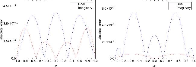
Figure 4. Absolute errors of the potential reconstructed by PPTS-PINNs in NLSE1 (left) and NLSE2 (right). |
Figure 5 displays the spatiotemporal distribution of the absolute error $\left|\hat{u}(x,t)-u(x,t)\right|$ between the inverted solution $\hat{u}(x,t)$ and the ground truth u(x, t) in the inverse problems of NLSE1 (left) and NLSE2 (right). The error is visualized via color maps over the domain (x, t) ∈ [-1, 1] × [0, 1]. It is evident that the error is primarily concentrated near boundaries and localized unstable regions, while the overall magnitude remains on the order of 10-3, indicating the model's strong solution reconstruction ability and excellent spatiotemporal fitting performance.
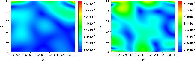
Figure 5. Absolute error distributions of the solution $\hat{u}(x,t)$ reconstructed by PPTS-PINNs with respect to the exact solution u(x, t) for NLSE1 (left) and NLSE2 (right). |
Figure 6 compares the inverted potentials ${\hat{V}}_{{\rm{re}}}(x)$ and ${\hat{V}}_{{\rm{im}}}(x)$ obtained by mPINNs with the corresponding reference potentials ${V}_{{\rm{re}}}(x)$ and ${V}_{{\rm{im}}}(x)$. Figure 7 illustrates the spatial distribution of their absolute errors, while figure 8 depicts the spatiotemporal error distribution between the inverted solution $\hat{u}(x,t)$ and the true solution u(x, t). These results indicate that, unlike PPTS-PINNs, the inversion obtained by mPINNs does not fully respect PT-symmetry, as evidenced by the asymmetric error distribution in figure 7.
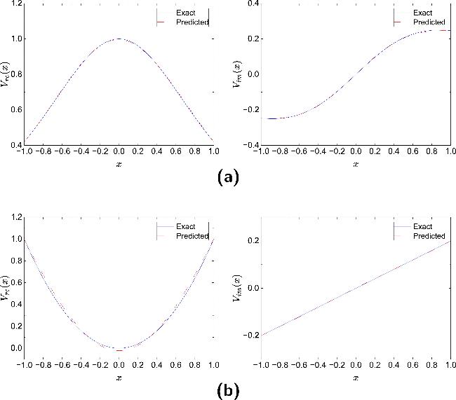
Figure 6. Comparison between the potential $\hat{V}(x)$ reconstructed by mPINNs and the exact potential V(x) in NLSE1 (a) and NLSE2 (b). |
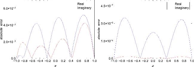
Figure 7. Absolute errors of the potential reconstructed by mPINNs in NLSE1 (left) and NLSE2 (right). |
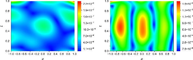
Figure 8. Absolute error distributions of the solution $\hat{u}(x,t)$ reconstructed by mPINNs with respect to the exact solution u(x, t) for NLSE1 (left) and NLSE2 (right). |
Table 3 summarizes the error metrics for both PPTS-PINNs and mPINNs, including the maximum norm error ($\ell$∞) and the relative $\ell$2 error (${\ell }_{2}^{{\rm{rel}}}$) for the real potential ${V}_{{\rm{re}}}(x)$, the imaginary potential ${V}_{{\rm{im}}}(x)$, and the solution u(x, t) in NLSE1 and NLSE2. Overall, all errors remain below the order of 10-3, with several cases reaching the order of 10-4.
Table 3. Error metrics for the real potential ${V}_{{\rm{re}}}$, imaginary potential ${V}_{{\rm{im}}}$, and solution u(x, t) using PPTS-PINNs and mPINNs. |
| Equation | Method | ${V}_{{\rm{re}}}(x)$ | ${V}_{{\rm{im}}}(x)$ | u(x, t) | |||
|---|---|---|---|---|---|---|---|
| $\ell$∞ | ${\ell }_{2}^{{\rm{r}}{\rm{e}}{\rm{l}}}$ | $\ell$∞ | ${\ell }_{2}^{{\rm{r}}{\rm{e}}{\rm{l}}}$ | $\ell$∞ | ${\ell }_{2}^{{\rm{r}}{\rm{e}}{\rm{l}}}$ | ||
| NLSE1 | PPTS-PINNs | 3.92 × 10⁻³ | 3.30 × 10⁻³ | 2.60 × 10⁻³ | 7.63 × 10⁻³ | 1.89 × 10⁻³ | 3.88 × 10⁻⁴ |
| mPINNs | 5.22 × 10⁻³ | 4.12 × 10⁻³ | 4.25 × 10⁻³ | 1.04 × 10⁻² | 2.25 × 10⁻³ | 5.34 × 10⁻⁴ | |
| NLSE2 | PPTS-PINNs | 5.51 × 10⁻³ | 6.88 × 10⁻³ | 5.37 × 10⁻⁴ | 3.29 × 10⁻³ | 1.46 × 10⁻³ | 5.72 × 10⁻⁴ |
| mPINNs | 3.48 × 10⁻² | 4.75 × 10⁻² | 1.81 × 10⁻³ | 9.09 × 10⁻³ | 1.60 × 10⁻³ | 9.93 × 10⁻⁴ | |
By comparing the results of the two methods, it is evident that PPTS-PINNs achieve higher inversion accuracy than mPINNs, particularly for the potential functions. This advantage is most pronounced in NLSE2, where both the $\ell$∞ and ${\ell }_{2}^{{\rm{rel}}}$ errors of ${V}_{{\rm{re}}}(x)$ and the $\ell$∞ error of ${V}_{{\rm{im}}}(x)$ are roughly an order of magnitude smaller for PPTS-PINNs. In contrast, the inversion accuracy for u(x, t) is comparable between the two methods, suggesting that the PT-symmetry constraint in PPTS-PINNs primarily enhances the accuracy of the potential function inversion without adversely affecting the solution reconstruction.
4.3. Inverse results with noisy data
This subsection presents the inversion results of the potential function V(x) in NLSE1 and NLSE2 using the PPTS-PINNs method combined with the gradient enhancement strategy under noise levels of 1% and 5%. These results aim to assess the method's performance in the presence of uncertain data. As defined in (14 ), the noise is applied individually to each exact observation u(xm, tm), so the specified percentages correspond to the relative value of each observation.
To assess the influence of training point numbers on model performance, we first conducted preliminary experiments varying the number of PDE residual points. These tests revealed that increasing PDE points can slightly improve the inversion performance of both PPTS-PINNs and mPINNs at the initial stage, but the improvement quickly saturates once a sufficient number of points is reached. In contrast, the reconstruction accuracy is much more sensitive to the noise level in the observational data. Considering that in practical applications acquiring additional observational data often incurs significant cost, we keep the number of observational data points fixed in our numerical experiments. When reporting the final results, we fixed a sufficiently large number of PDE points to ensure training stability and focused on two representative noise levels (1% and 5%). Only under higher noise conditions did we introduce additional PDE points to maintain robustness.
Based on these insights, table 4 summarizes the hyperparameter configurations and sample sizes for PPTS-PINNs applied to NLSE1 and NLSE2 under varying noise levels (1% and 5%). The table lists the number of hidden layers and the width of each layer for the three subnetworks: ${\hat{u}}^{\theta }$, ${\hat{V}}_{{\rm{re}}}^{\theta }$, and ${\hat{V}}_{{\rm{im}}}^{\theta }$. All sampling points are generated using a uniform mesh and remain fixed throughout the training process. To enhance the model's robustness under higher noise levels, we appropriately increase the number of training points outside the observation set ${{ \mathcal T }}_{m}$, including PDE residual points ${{ \mathcal T }}_{p}$, boundary points ${{ \mathcal T }}_{b}^{l}\cup {{ \mathcal T }}_{b}^{r}$, initial condition points ${{ \mathcal T }}_{i}$, and gradient loss points ${{ \mathcal T }}_{g}$. Among these, ${{ \mathcal T }}_{p}={{ \mathcal T }}_{g}$ and ${{ \mathcal T }}_{m}\subset {{ \mathcal T }}_{g}$, ensuring the effective propagation of gradient information. This strategy aims to suppress the interference of noise in the inversion process by introducing more informative training points, thereby improving the inversion accuracy.
Table 4. Summary of hyperparameters, sampling sizes for PPTS-PINNs applied to NLSE1 and NLSE2 under varying noise levels (1% and 5%). |
| Equation | Hidden layers | Width | $\left|{{ \mathcal T }}_{p}\right|$ | $\left|{{ \mathcal T }}_{b}^{l}\cup {{ \mathcal T }}_{b}^{r}\right|$ | $\left|{{ \mathcal T }}_{i}\right|$ | $\left|{{ \mathcal T }}_{m}\right|$ | $\left|{{ \mathcal T }}_{g}\right|$ | ||||
|---|---|---|---|---|---|---|---|---|---|---|---|
| ${\hat{u}}^{\theta }$ | ${\hat{V}}_{{\rm{re}}}^{\theta }$ | ${\hat{V}}_{{\rm{im}}}^{\theta }$ | ${\hat{u}}^{\theta }$ | ${\hat{V}}_{{\rm{re}}}^{\theta }$ | ${\hat{V}}_{{\rm{im}}}^{\theta }$ | ||||||
| NLSE1 (1% noise) | 4 | 4 | 4 | 32 | 32 | 32 | 3440 | 800 | 800 | 860 | 3440 |
| NLSE2 (1% noise) | 3 | 3 | 3 | 32 | 32 | 32 | 3440 | 800 | 800 | 860 | 3440 |
| NLSE1 (5% noise) | 4 | 4 | 4 | 64 | 32 | 32 | 7740 | 1600 | 1600 | 860 | 7740 |
| NLSE2 (5% noise) | 3 | 3 | 3 | 64 | 32 | 32 | 7740 | 1600 | 1600 | 860 | 7740 |
In addition, inspired by the idea of scaling network capacity to improve model expressiveness [27], we increased the width of the potential function networks ${\hat{V}}_{{\rm{re}}}^{\theta }$ and ${\hat{V}}_{{\rm{im}}}^{\theta }$ to 32. When the training set is larger or under high-noise conditions, the main network ${\hat{u}}^{\theta }$ is widened from 32 to 64 to better capture the information in the dataset.
Table 5 reports the computational times corresponding to the configurations in table 4, along with the number of trainable parameters and training epochs. As expected, the training time increases with network depth, width, and the number of sampling points, reflecting the direct correlation between model complexity and computational cost. Notably, PPTS-PINNs generally require longer training times than mPINNs, despite having fewer parameters, mainly due to the gradient enhancement strategy, which introduces additional computations during training.
Table 5. Comparison of computational times for PPTS-PINNs and mPINNs under varying noise levels (1% and 5%), along with parameter counts and training epochs. |
| Equation | Method | Parameters | Epochs | Time (s) |
|---|---|---|---|---|
| NLSE1 (1% noise) | PPTS-PINNs | 9860 | 30 000 | 3750 |
| mPINNs | 28 612 | 30 000 | 582 | |
| NLSE2 (1% noise) | PPTS-PINNs | 6692 | 30 000 | 5225 |
| mPINNs | 19 300 | 30 000 | 678 | |
| NLSE1 (5% noise) | PPTS-PINNs | 19 332 | 30 000 | 3762 |
| mPINNs | 50 436 | 30 000 | 749 | |
| NLSE2 (5% noise) | PPTS-PINNs | 13 060 | 30 000 | 5579 |
| mPINNs | 33 924 | 30 000 | 975 |
Figures 9 and 10 demonstrate the comparison between inverted potential functions V(x) and ground truth solutions under 1% and 5% noise levels for NLSE1 and NLSE2, respectively. Each group contains left panels showing real component comparisons (${\hat{V}}_{{\rm{re}}}(x)$ versus ${V}_{{\rm{re}}}(x)$) and right panels displaying imaginary component comparisons (${\hat{V}}_{{\rm{im}}}(x)$ versus ${V}_{{\rm{im}}}(x)$). Despite moderate noise disturbances, the inversion results remain closely aligned with the true solution curves, validating PPTS-PINNs' effectiveness in complex data environments.
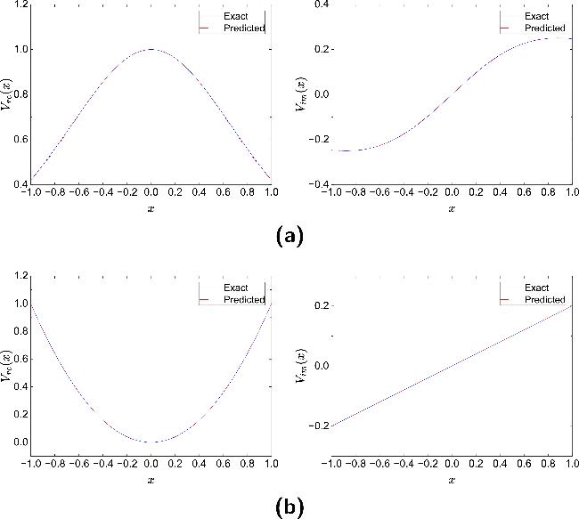
Figure 9. Comparison between the potential $\hat{V}(x)$ reconstructed by PPTS-PINNs and the exact potential V(x) in NLSE1 (a) and NLSE2 (b) under 1% noise level. |
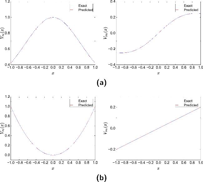
Figure 10. Comparison between the potential $\hat{V}(x)$ reconstructed by PPTS-PINNs and the exact potential V(x) in NLSE1 (a) and NLSE2 (b) under 5% noise level. |
Figure 11 presents spatial distributions of inversion errors for potential functions under 1% (left) and 5% (right) noise levels, with panel (a) for NLSE1 and panel (b) for NLSE2. We observe increased errors in both real and imaginary components with stronger noise, particularly more pronounced in real components. Nevertheless, overall errors remain controlled within the order of 10-3, demonstrating strong noise resistance of the method.
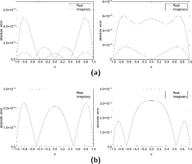
Figure 11. Absolute error distributions of the potential reconstructed by PPTS-PINNs in NLSE1 (a) and NLSE2 (b) under different noise levels. Left: 1% noise; right: 5% noise. |
Figure 12 displays spatiotemporal absolute error distributions between inverted solutions $\hat{u}(x,t)$ and true solutions u(x, t) under different noise levels, with panel (a) for NLSE1 and panel (b) for NLSE2. At 1% noise level, errors primarily concentrate near boundaries and local nonstationary regions. Under 5% noise conditions, errors increase slightly but maintain magnitudes within 10-3, indicating PPTS-PINNs' capability to effectively reconstruct solution functions u(x, t) from noisy observational data.
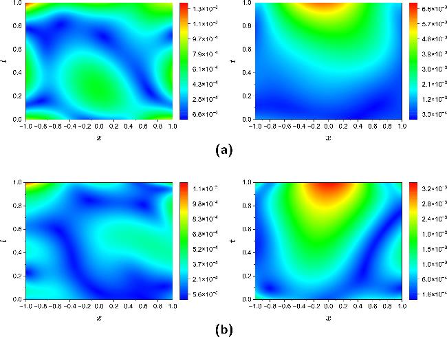
Figure 12. Absolute error distributions of the solution $\hat{u}(x,t)$ reconstructed by PPTS-PINNs with respect to the exact solution u(x, t) in NLSE1 (a) and NLSE2 (b) under different noise levels. Left: 1% noise; right: 5% noise. |
The inversion results obtained by mPINNs are shown in figures 13 and 14, displaying ${\hat{V}}_{{\rm{re}}}(x)$ and ${\hat{V}}_{{\rm{im}}}(x)$ at 1% and 5% noise levels. The spatial distribution of absolute errors in the inverted potentials and the spatiotemporal error distribution of the solution u(x, t) are presented in figures 15 and 16, respectively.
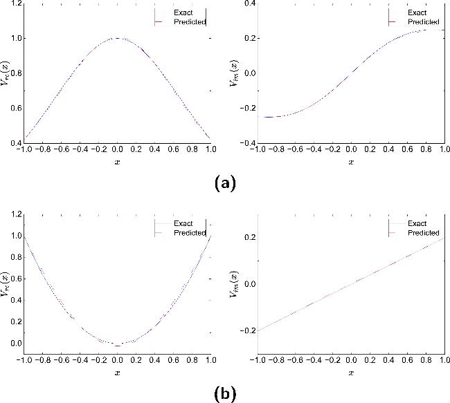
Figure 13. Comparison between the potential $\hat{V}(x)$ reconstructed by mPINNs and the exact potential V(x) in NLSE1 (a) and NLSE2 (b) under 1% noise level. |
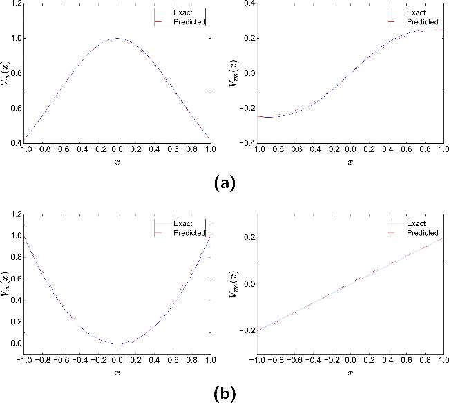
Figure 14. Comparison between the potential $\hat{V}(x)$ reconstructed by mPINNs and the exact potential V(x) in NLSE1 (a) and NLSE2 (b) under 5% noise level. |
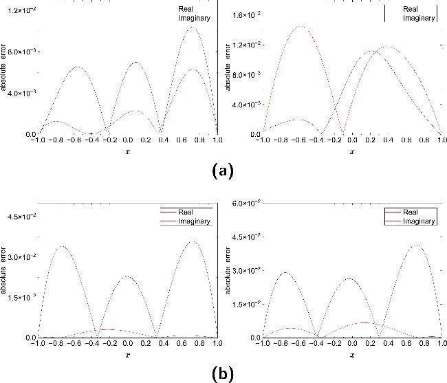
Figure 15. Absolute error distributions of the potential reconstructed by mPINNs in NLSE1 (a) and NLSE2 (b) under different noise levels. Left: 1% noise; right: 5% noise. |
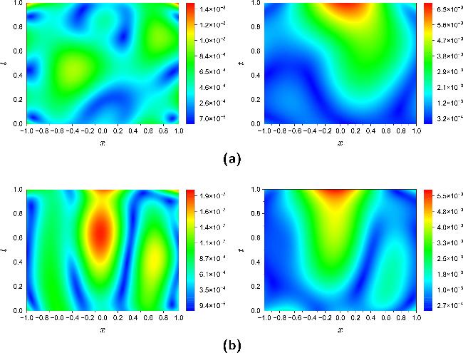
Figure 16. Absolute error distributions of the solution $\hat{u}(x,t)$ reconstructed by mPINNs with respect to the exact solution u(x, t) in NLSE1 (a) and NLSE2 (b) under different noise levels. Left: 1% noise; right: 5% noise. |
A comprehensive comparison of error metrics for both PPTS-PINNs and mPINNs is provided in table 6. PPTS-PINNs consistently achieves substantially smaller errors than mPINNs for the inversion of the real and imaginary potential functions (${V}_{{\rm{re}}}(x)$ and ${V}_{{\rm{im}}}(x)$) across all test cases and noise levels. For the solution u(x, t), the errors of PPTS-PINNs and mPINNs are generally comparable, with only minor differences observed. Across different equations and noise levels, the errors in ${V}_{{\rm{re}}}(x)$ and ${V}_{{\rm{im}}}(x)$ obtained by PPTS-PINNs are often one to two orders of magnitude smaller than those of mPINNs, highlighting the method's superior robustness and accuracy in recovering the potential functions under noisy data conditions.
Table 6. Error metrics for the real potential ${V}_{{\rm{re}}}$, imaginary potential ${V}_{{\rm{im}}}$, and solution u(x, t) under varying noise levels (1% and 5%), using PPTS-PINNs and mPINNs. |
| Equation | Method | ${V}_{{\rm{re}}}(x)$ | ${V}_{{\rm{im}}}(x)$ | u(x, t) | |||
|---|---|---|---|---|---|---|---|
| $\ell$∞ | ${\ell }_{2}^{{\rm{r}}{\rm{e}}{\rm{l}}}$ | $\ell$∞ | ${\ell }_{2}^{{\rm{r}}{\rm{e}}{\rm{l}}}$ | $\ell$∞ | ${\ell }_{2}^{{\rm{r}}{\rm{e}}{\rm{l}}}$ | ||
| NLSE1 (1% noise) | PPTS-PINNs | 5.07 × 10⁻³ | 3.35 × 10⁻³ | 1.48 × 10⁻³ | 4.61 × 10⁻³ | 1.39 × 10⁻³ | 4.67 × 10⁻⁴ |
| mPINNs | 1.04 × 10⁻² | 7.24 × 10⁻³ | 6.31 × 10⁻³ | 1.42 × 10⁻² | 1.48 × 10⁻³ | 5.96 × 10⁻⁴ | |
| NLSE2 (1% noise) | PPTS-PINNs | 2.26 × 10⁻³ | 3.41 × 10⁻³ | 6.63 × 10⁻⁵ | 4.06 × 10⁻⁴ | 1.14 × 10⁻³ | 3.08 × 10⁻⁴ |
| mPINNs | 3.59 × 10⁻² | 4.89 × 10⁻² | 3.13 × 10⁻³ | 1.40 × 10⁻² | 1.94 × 10⁻³ | 1.14 × 10⁻³ | |
| NLSE1 (5% noise) | PPTS-PINNs | 6.03 × 10⁻³ | 6.55 × 10⁻³ | 1.75 × 10⁻³ | 6.01 × 10⁻³ | 6.29 × 10⁻³ | 2.53 × 10⁻³ |
| mPINNs | 1.12 × 10⁻² | 7.52 × 10⁻³ | 1.45 × 10⁻² | 4.83 × 10⁻² | 6.68 × 10⁻³ | 2.74 × 10⁻³ | |
| NLSE2 (5% noise) | PPTS-PINNs | 3.20 × 10⁻³ | 4.77 × 10⁻³ | 8.63 × 10⁻⁵ | 5.34 × 10⁻⁴ | 3.38 × 10⁻³ | 1.65 × 10⁻³ |
| mPINNs | 4.15 × 10⁻² | 5.16 × 10⁻² | 6.79 × 10⁻³ | 3.28 × 10⁻² | 5.76 × 10⁻³ | 2.54 × 10⁻³ | |
In summary, although the gradient enhancement strategy increases the training time of PPTS-PINNs, it substantially improves robustness under noisy conditions by effectively mitigating the influence of data perturbations on potential function inversion, demonstrating the method's superior generalization and accuracy performance.
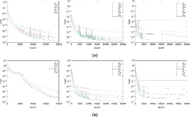
Figure 17 and table 7 illustrate the evolution trends and final values of various loss components during training. Under noise-free conditions, all sub-loss terms exhibit a smooth decreasing trend, indicating good convergence behavior of the model. Under high-noise conditions, some loss components (such as ${{ \mathcal L }}_{p}$ and ${{ \mathcal L }}_{g}$) display noticeable fluctuations in the early stages of training but still converge overall.
Figure 17. Loss function curves of the PPTS-PINNs method during training for NLSE1 (a) and NLSE2 (b) under different noise levels. Left: exact data (no noise); middle: 1% noise; right: 5% noise. The curves show the evolution of individual loss components over epochs. |
Table 7. Final values of individual loss components of the PPTS-PINNs method for NLSE1 and NLSE2 under varying noise levels. Missing entries are indicated by '——'. |
| Equation | ${{ \mathcal L }}_{p}$ | ${{ \mathcal L }}_{b}$ | ${{ \mathcal L }}_{i}$ | ${{ \mathcal L }}_{m}$ | ${{ \mathcal L }}_{g}$ | ${ \mathcal L }$ |
|---|---|---|---|---|---|---|
| NLSE1 | 3.29 × 10⁻⁶ | 6.44 × 10⁻⁷ | 1.79 × 10⁻⁷ | 5.75 × 10⁻⁷ | —— | 4.69 × 10⁻⁶ |
| NLSE2 | 1.54 × 10⁻⁵ | 1.39 × 10⁻⁶ | 6.20 × 10⁻⁷ | 7.68 × 10⁻⁷ | —— | 1.82 × 10⁻⁵ |
| NLSE1 (1% noise) | 1.18 × 10⁻⁷ | 6.95 × 10⁻⁷ | 2.58 × 10⁻⁷ | 7.78 × 10⁻⁵ | 9.27 × 10⁻⁶ | 8.81 × 10⁻⁵ |
| NLSE2 (1% noise) | 1.12 × 10⁻⁷ | 1.22 × 10⁻⁶ | 4.83 × 10⁻⁷ | 6.40 × 10⁻⁵ | 1.01 × 10⁻⁵ | 7.59 × 10⁻⁵ |
| NLSE1 (5% noise) | 1.55 × 10⁻⁷ | 1.16 × 10⁻⁶ | 1.14 × 10⁻⁶ | 1.93 × 10⁻³ | 7.35 × 10⁻⁶ | 1.94 × 10⁻³ |
| NLSE2 (5% noise) | 4.61 × 10⁻⁷ | 2.57 × 10⁻⁶ | 2.20 × 10⁻⁶ | 1.58 × 10⁻³ | 3.16 × 10⁻⁵ | 1.62 × 10⁻³ |
The results in table 7 further demonstrate that although the introduction of noise increases the overall loss level, most sub-loss components remain stable within the range of 10-6-10-5. Among them, the PDE residual loss ${{ \mathcal L }}_{p}$, boundary loss ${{ \mathcal L }}_{b}$, and initial condition loss ${{ \mathcal L }}_{i}$ show relatively small variations across different noise levels, suggesting that the model maintains good stability under key physical constraints. Notably, the observation loss ${{ \mathcal L }}_{m}$ is particularly sensitive to noise, rising significantly from the order of 10-7 in the noise-free case to 10-3 under high noise conditions. This phenomenon indicates that ${{ \mathcal L }}_{m}$ tends to accumulate observation errors in high-noise environments. However, the incorporation of PT-symmetry constraints and the gradient enhancement strategy effectively mitigates this error propagation, thereby significantly improving the robustness and reliability of the overall inversion framework.
5. Conclusion
The proposed PPTS-PINNs method demonstrates excellent performance in solving the inverse problem of NLSEs with complex-valued latent variables. Under noise-free conditions, the model can stably and accurately reconstruct both the real and imaginary parts of the potential function V(x), while successfully recovering the distribution of the solution function u(x, t) across the entire spatiotemporal domain. Through systematic numerical experiments, we further evaluate the error distribution and robustness of the model under different levels of observational noise (1% and 5%).
Experimental results demonstrate that the PT-symmetry constraint and the gradient enhancement strategy play a crucial role in improving model stability and inversion accuracy, particularly under high-noise conditions, where they significantly suppress the propagation of observational errors. Although some error metrics slightly increase with higher noise levels, the overall error remains within the order of 10-3, confirming the noise robustness and generalization capability of the proposed PPTS-PINNs method. In addition, the introduction of a composite scaling strategy for neural network architecture tuning effectively enhances both the expressiveness and convergence of the model. However, the gradient enhancement strategy requires the computation of higher-order derivatives during training, which considerably increases the computational cost.
In summary, PPTS-PINNs demonstrate strong capability to integrate physical constraints, PT-symmetric structures, and gradient enhancement mechanisms, providing a stable and highly generalizable deep learning framework for solving inverse problems of potential functions with noise. In future work, the mathematical structure of PT-symmetry in high-dimensional spaces could be further explored to construct more generalizable symmetry constraints, thereby extending the method to more complex systems in higher dimensions to meet the diverse demands of physical and engineering modeling. Moreover, performance improvements could be achieved by incorporating advanced residual point sampling strategies [28] and adaptive weighting schemes [24] for different loss terms In addition, recent deep learning architectures, such as the TP-Bi_LSTM RNN [29] and the dual-channel CRNN [30] designed for modeling complex soliton dynamics, could be considered to replace or enhance the subnetworks in PPTS-PINNs, potentially offering stronger capabilities for capturing nonlinear and multiscale features in related inverse problems.