


1. Introduction
The Benney-Roskes-Davey-Stewartson equation is a well-known model to describe the evolution of a (2+1)-dimensional wave packet on water of finite depth [1-3]. This equation becomes integrable under the shallow water approximation [3], and is sometimes termed the Davey-Stewartson (DS) equation. The DS equation has received considerable attention from the physics and mathematics communities as a prototype model of nonlinear interactions between long and short waves. In addition, this equation can also be obtained from a self-dual Yang-Mills equation via a suitable reduction technique [4]. Depending on the strength of surface tension, the DS equation can be divided into two types [3]: DSI equation (strong surface tension) and DSII equation (weak surface tension). This paper focuses on the Davey-Stewartson I (DSI) equation, which can be expressed in the following form
$\begin{eqnarray}\left\{\begin{array}{l}{\rm{i}}{A}_{t}={A}_{xx}+{A}_{yy}+(\epsilon | A{| }^{2}-2Q)A,\\ {Q}_{xx}-{Q}_{yy}=\epsilon {(| A{| }^{2})}_{xx},\end{array}\right.\end{eqnarray}$
where ε = ±1 is the sign of nonlinearity, A ≡ A(x, y, t) is a complex function representing the envelope of the surface wave packet, and Q ≡ Q(x, y, t) is a real function that represents the potential of the velocity field in the (2+1)-dimensional surface water wave context.Rogue waves are exceptionally large and unpredictable ocean surface waves that may cause danger to ships in the sea [5]. Due to their mysterious nature and potential damage, rogue waves have received intensive experimental and theoretical studies. Currently, they are at the frontier of research in diverse physical fields, including water wave tank [6, 7], optical fibers [8, 9], Bose-Einstein condensates [10], plasma physics [11], acoustics [12] and superfluid helium [13]. So far, theoretical studies on rogue waves have focused mostly on (1+1)-dimensional models, such as in the nonlinear Schrödinger (NLS) equation [14-18], the Manakov system [19-22], the massive thirring model [23], the three-wave resonant interaction model [24], and many others [25].
It is quite meaningful to investigate rogue wave patterns for (2+1)-dimensional equations since surface waves in the ocean are always governed via (2+1)-dimensional models. Given that the DS equation is a well-known mathematical model which arises in the description of two-dimensional surface water waves, the pattern formation of DS rogue wave solutions could have significant implications for the investigation of rogue waves in the ocean. Previously, rogue waves in DSI have been derived using the Hirota bilinear method [26]. It was found that rogue waves primarily exhibit wave crests in line-shaped and nonlinear interaction of multi-line in two-dimensional spatial plane. Recently, varieties of rogue curves in the DSI equation have been reported [27]. The wave crests for these rogue curves can exhibit shapes of closed or open curves in the spatial plane. They arise from a uniform background when time $t={ \mathcal O }(1)$, and then reach high amplitude in various attractive shapes, such as a closed ring, a knotted curve, and many others. Moreover, it has been found that such two-dimensional curved-shape rogue wave patterns would appear when an internal parameter in bilinear rogue waves expressions are real and large [27]. The emergence of these new and striking shapes of rogue curves provide more potential possibilities for extreme physical events in nature and experimentation.
In particular, we further observe that these rogue curves always appear possibly with a few lumps on the background. As time progresses, those lumps would not disappear into the same constant background without trace. Instead, they will evolve into several localized lump waves on the constant background that persist at large time, thus leaving with a trace. Due to these peculiar behaviors, an interesting problem for us is to investigate large-time asymptotic wave dynamics and pattern formation for DSI rogue curves. Especially, when time is large, the (x, y) locations as well as the dynamic behavior for these lump-shaped waves are still unclear.
In this paper, we study asymptotic wave dynamics for rogue curves in the DSI equation through large-time asymptotic analysis on its rogue wave solutions. This work is motivated by earlier work on wave patterns of higher-order lumps of the Kadomtsev-Petviashvili I equation, where it is shown that fascinating lump patterns appear at a large time, which are described analytically by root structures of the Yablonskii-Vorob'ev polynomials and the Wronskian-Hermite polynomials. For rogue curves in the context of the DSI equation, we will demonstrate that when time is large, a certain number of lumps would appear on the uniform background, exhibiting various wave patterns. We further show that such wave patterns and the numbers of these lumps can be determined by structure of nonzero roots of the Wronskian-Hermite polynomials. More importantly, as time increases, we find that individual lump-shaped wave would asymptotically change into a line-shaped soliton, undergoing a state change. We compare our asymptotic predictions to true solutions and demonstrate excellent agreement between them.
This paper is organized as follows. In section 2 , we introduce the explicit bilinear rogue wave solutions in the DSI equation. By choosing different parameters, we show various wave patterns and their dynamics for DSI rogue curves at large times. In section 3 , we present our main results on the asymptotic wave dynamics of rogue curves when time becomes large, including their connections with root structures of the Wronskian-Hermite polynomials. In section 4 , we graphically and quantitatively compare our analytical predictions and true solutions. In section 5 , we prove the theorem presented in section 4 of this paper for p = 1 case. In section 6 , we briefly discuss large-time asymptotics for DSI rogue curves when p ≠ 1. Section 7 summarizes the paper with some discussions.
2. Pattern dynamics of rogue curves at large times
General rogue wave solutions for equation (1 ) have been derived in terms of differential operators [26]. More explicit representations of DSI rogue waves have been provided and proved [27]. Specifically, the Davey-Stewartson I equation (1 ) admits the following general higher-order non-singular rational solutions [27]:
$\begin{eqnarray}{A}_{{\rm{\Lambda }}}(x,y,t)=\sqrt{2}\frac{g}{f},\end{eqnarray}$
$\begin{eqnarray}{Q}_{{\rm{\Lambda }}}(x,y,t)=1-2\epsilon {\left(\mathrm{log}f\right)}_{xx},\end{eqnarray}$
where f ≡ f(x, y, t) is a real function, g ≡ g(x, y, t) is a complex function, and $\Lambda$ = (n1, n2, …, nN) denotes an order-index vector. Here, N is the length of vector $\Lambda$, each ni is a nonnegative integer, and n1 < n2 < … < nN. To describe the solution, we introduce a tau function as follows $\begin{eqnarray}f={\tau }_{0},\quad g={\tau }_{1},\end{eqnarray}$
$\begin{eqnarray}{\tau }_{k}=\mathop{\det }\limits_{1\leqslant i,j\leqslant N}\left({\phi }_{i,j}^{(k)}\right),\end{eqnarray}$
the matrix elements ${\phi }_{i,j}^{(k)}$ of Γk are defined by $\begin{eqnarray*}\begin{array}{rcl}{\phi }_{i,j}^{(k)} & = & \displaystyle \sum _{\nu =0}^{\min ({n}_{i},{n}_{j})}\frac{1}{{4}^{\nu }}{S}_{{n}_{i}-\nu }[{{\boldsymbol{x}}}^{+}(k)+\nu {\boldsymbol{s}}]\\ & & \times {S}_{{n}_{j}-\nu }[{{\boldsymbol{x}}}^{-}(k)+\nu {\boldsymbol{s}}],\end{array}\end{eqnarray*}$
where the vectors ${{\boldsymbol{x}}}^{\pm }(k)=\left({x}_{1}^{\pm },{x}_{2}^{\pm },\cdots \,\right)$ are $\begin{eqnarray}\begin{array}{rcl}{x}_{r}^{+}(k) & = & \frac{{(-1)}^{r}}{r!p}{x}_{-1}+\frac{{(-2)}^{r}}{r!{p}^{2}}{x}_{-2}\\ & & +\frac{1}{r!}p{x}_{1}+\frac{{2}^{r}}{r!}{p}^{2}{x}_{2}+k{\delta }_{r,1}+{a}_{r},\end{array}\end{eqnarray}$
$\begin{eqnarray}\begin{array}{rcl}{x}_{r}^{-}(k) & = & \frac{{(-1)}^{r}}{r!p}{x}_{-1}+\frac{{(-2)}^{r}}{r!{p}^{2}}{x}_{2}\\ & & +\frac{1}{r!}p{x}_{1}+\frac{{2}^{r}}{r!}{p}^{2}{x}_{-2}-k{\delta }_{r,1}+{a}_{r}^{* },\end{array}\end{eqnarray}$
with $\begin{eqnarray}\begin{array}{rcl}{x}_{1} & = & \frac{1}{2}(x+y),\,\,{x}_{-1}=\frac{1}{2}\epsilon (x-y),\\ {x}_{2} & = & -\frac{1}{2}{\rm{i}}t,\,\,{x}_{-2}=\frac{1}{2}{\rm{i}}t.\end{array}\end{eqnarray}$
Here, p ≠ 0 is a real constant, δr,1 is the Kronecker delta function defined as ${\delta }_{r,1}=\left\{\begin{array}{ll}1, & r=1\\ 0, & r\ne 1\end{array}\right.$.The vector s = (0, s2, 0, s4, …) consists of coefficients from the expansion
$\begin{eqnarray}\mathrm{ln}\left[\frac{2}{\kappa }\tanh \frac{\kappa }{2}\right]=\displaystyle \sum _{r=1}^{\infty }{s}_{r}{\kappa }^{r}.\end{eqnarray}$
And ${a}_{1},{a}_{2},\ldots ,{a}_{{n}_{N}}$ are free complex internal parameters. The elementary Schur polynomials Sn(x) with x = (x1, x2, …) are generated by the function $\begin{eqnarray}\displaystyle \sum _{n=0}^{\infty }{S}_{n}({\boldsymbol{x}}){\epsilon }^{n}=\exp \left(\displaystyle \sum _{k=1}^{\infty }{x}_{k}{\epsilon }^{k}\right),\end{eqnarray}$
and we define Sn ≡ 0 when n < 0.The above bilinear expressions have been derived in [27]. The first element a1 can be further absorbed through a coordinate shift into (x, t) or (y, t). Moreover, It is observed that equation (1 ) remains invariant under the variable transformation of Q → Q + ε|A|2, x ↔ y, and ε → -ε. Thus, we set ε = 1, a1 = 0 in the general solutions (2 )-(3 ) without losing generality, and denote ${\boldsymbol{a}}=(0,{a}_{2},\ldots ,{a}_{{n}_{N}})$ as a vector of irreducible internal free parameters.
Firstly, let us consider a special case where the index vector $\Lambda$ is given by (1, 3, 5, …, 2N - 1). In this case, it is found that the corresponding solution is a typical higher-order line-shaped rogue wave. To demonstrate these rogue waves in DSI, we show one example. By choosing N = 5 in solution (2 ) with
$\begin{eqnarray}p=1,\quad {\rm{\Lambda }}=(1,3,5,7,9),\quad {\boldsymbol{a}}={\bf{0}}.\end{eqnarray}$
The corresponding solution |A$\Lambda$(x, y, t)| at four time values of t = 0, 1, 3 and 10 is plotted in figure 1.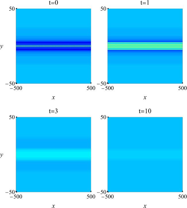
Figure 1. A higher-order line-shaped rogue wave (|A|) in the DSI equation at four time values of t = 0, 1, 3 and 10 for parameter choices in equation ( |
It is seen that a line-shaped rogue wave appears at t = 0, reaching peak amplitude of $11\sqrt{2}$. At the intermediate time of t = 1, the wave crests form a multi-line structure, and then it begins to disappear and becomes nearly invisible at t = 3. At the large times, the solution disappears into the constant background without trace (see t = 10 panel). Such types of rogue wave solutions are not the main focus of this paper. Here, we just briefly mention it without further discussion.
Next, we consider the general case where the index vector ${\rm{\Lambda }}\ne \left(1,3,5,\cdots 2N-1\right)$. In this case, to demonstrate large-time asymptotic wave dynamics of rogue curves in DSI equation, we will illustrate three examples. In all these examples, we will restrict p = 1.
For the first example, we take N = 2, and choose the index vector as well as the internal parameters in equations (4 )-(5 ) as
$\begin{eqnarray}{\rm{\Lambda }}=(1,4),\quad {\boldsymbol{a}}=(0,0,0,1000).\end{eqnarray}$
The graphs of solution |A$\Lambda$(x, y, t)| at three time values of t = 0, 2, 5 are depicted in the upper row of figure 2.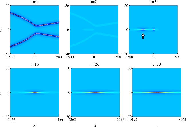
Figure 2. A DSI rogue curve (|A$\Lambda$(x, y, t)|) for parameter choices of ( |
It is observed that a rogue wave emerges from the uniform background in the (x, y) plane, which consists of two symmetric curves with respect to the x-axis, attaining its peak amplitude of $3\sqrt{2}$ at t = 0. This t = 0 panel in figure 2 has been reported in [27] for a larger parameter value. As time gets large, these rogue curves firstly retreats to the same uniform background at t = 2. And then, there are two lump-shaped waves with different sizes and shapes arise from the constant background at a larger time value of t = 5, which is an interesting feature we should notice. As time evolves, these two lumps move to the left and right along the horizontal direction, separately.
To better observe their shape changes over time, we focus on one of these two individual lumps (the one marked by a white arrow in the upper rightmost panel of figure 2, at t = 5), and show its asymptotic sates at large time values. More specifically, we plot true solution |A$\Lambda$(x, y, t)| at three time points of t = 10, 20, and 30 in the lower row of figure 2. Visually, it is seen that as time increases, the width of this lump extends along the x-axis, and the lump-shaped wave gradually becomes a line soliton. While the other lump wave would exhibit similar dynamical behaviors when time gets large, graphs of time evolution for that lump are omitted brevity.
For the second example, we choose N = 2, and set parameters as2 ) at three time values t = 0, 3 and 8 is depicted in the upper row of figure 3.
$\begin{eqnarray}{\rm{\Lambda }}=(2,3),\quad {\boldsymbol{a}}=(0,0,300).\end{eqnarray}$
The corresponding true solution |A$\Lambda$(x, y, t)| from equation (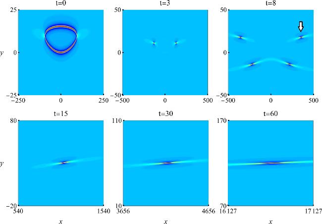
Figure 3. A DSI rogue curve (|A$\Lambda$(x, y, t)|) for parameter choices of ( |
It is seen that a ring-shaped rogue wave appears at t = 0, with its crests forming a closed curve, reaching a peak amplitude of $3\sqrt{2}$. This t = 0 panel in figure 3 has also been reported in [27] for a larger parameter value. Then, this rogue ring begins to disappear and becomes invisible at t = 3, with two lumps staying on the uniform background. Shortly afterward, these two lumps split into four lump-shaped waves at a larger time value of t = 8. As time evolves, these lumps move along four opposite directions in the (x, y) plane. To better trace their locations and asymptotic sates when time is getting large, we focus on one of these four lumps, which is marked by a white arrow in figure 3 at t = 8 (while the other three lumps would exhibit the same behavior), and plot true solutions |A$\Lambda$(x, y, t)| at three time values of t = 15, 30 and 60 in the lower row of figure 3. Then, it can be observed that as time evolves, the shape as well as the orientation of this lump is varying, and it gradually becomes a line soliton on a constant background.
For the third example, we choose N = 3 with parameters
$\begin{eqnarray}{\rm{\Lambda }}=(2,3,4),\quad {\boldsymbol{a}}=(0,0,0,1000).\end{eqnarray}$
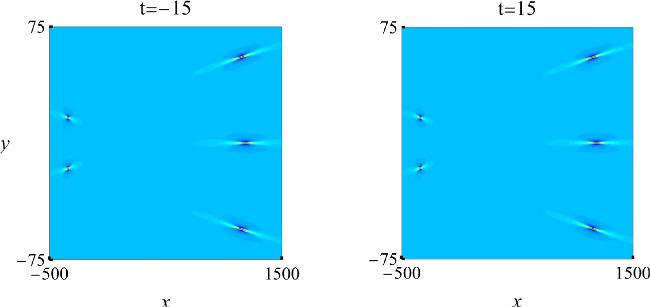
The corresponding true solution |A$\Lambda$(x, y, t)| at three time values t = -15, 0 and 15 is depicted in figure 4.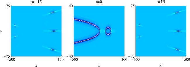
Figure 4. A DSI rogue curve (|A$\Lambda$(x, y, t)|) for parameter choices of ( |
It is seen that a parabola-shaped rogue curve combined with a ring-shaped rogue wave appears at t = 0. This striking wave pattern has not been reported before. Then, at two symmetric large times t = -15 and t = 15, from the overview perspective, this solution splits up into five lump waves arranged in a quasi-trapezoid shape. For each lump wave, when time gets even larger, it would gradually evolve into a line soliton on constant background. Similar to what has been observed in figures 2 and 3.
Moreover, it is noted that in the above examples, both solutions satisfy the time-reversal symmetry
$\begin{eqnarray*}{A}_{{\rm{\Lambda }}}(x,y,-t)={[{A}_{{\rm{\Lambda }}}(x,y,t)]}^{* },\end{eqnarray*}$
thus |A$\Lambda$(x, y, t)| = |A$\Lambda$(x, y, - t)|. Due to this property, we only need to discuss asymptotic wave dynamics for large positive time in such examples.How can we understand the large-time asymptotic wave dynamics of these rogue curves? In particular, how to analytically predict these shape changes and (x, y) locations for these lump-shaped waves at large times? These will be explained in the following section.
3. Asymptotic wave dynamics of rogue curves at large times
It is revealed that the large-time asymptotic wave dynamics of these rogue curves can be predicted by roots structure of the Wronskian-Hermite polynomials. So we first introduce such polynomials and their roots structure.
Let qk(z) be the polynomial defined by
$\begin{eqnarray}\displaystyle \sum _{k=0}^{\infty }{q}_{k}(z){\epsilon }^{k}=\exp \left(z\epsilon +{\epsilon }^{2}\right),\end{eqnarray}$
and qk(z) ≡ 0 if k < 0. These qk(z) polynomials are related to Hermit polynomials through simple variable transformations. Then the Wronskian-Hermite polynomial W$\Lambda$(z) is given by the following Wronskian determinant $\begin{eqnarray*}{W}_{{\rm{\Lambda }}}(z)=\left|\begin{array}{cccc}{q}_{{n}_{1}}(z) & {q}_{{n}_{1}-1}(z) & \cdots \, & {q}_{{n}_{1}-N+1}(z)\\ {q}_{{n}_{2}}(z) & {q}_{{n}_{2}-1}(z) & \cdots \, & {q}_{{n}_{2}-N+1}(z)\\ \vdots & \vdots & \ddots & \vdots \\ {q}_{{n}_{N}}(z) & {q}_{{n}_{N}-1}(z) & \cdots \, & {q}_{{n}_{N}-N+1}(z)\end{array}\right|,\end{eqnarray*}$
where $\Lambda$ = (n1, n2, …, nN) is the index vector with {ni} being positive and distinct integers arranged in ascending order.Regarding root structures of Wronskian-Hermite polynomials W$\Lambda$(z), the following facts hold:
1. The degree of polynomial W$\Lambda$(z) is equivalent to ρ, where ρ is defined as
$\begin{eqnarray}\rho =\displaystyle \sum _{i=1}^{N}{n}_{i}-\frac{N(N-1)}{2}.\end{eqnarray}$
2. The multiplicity of the zero root in W$\Lambda$(z) is $\frac{d(d+1)}{2}$, where d = kodd - keven, and kodd, keven represent the numbers of odd and even elements in the index vector $\Lambda$, respectively. The number of nonzero roots in W$\Lambda$(z), denoted as Nw, equals to
$\begin{eqnarray}{N}_{w}=\rho -\frac{d(d+1)}{2}.\end{eqnarray}$
3. The quartet root symmetry: If z0 is a root of W$\Lambda$(z), then -z0, ${z}_{0}^{* }$, and $-{z}_{0}^{* }$ are also roots.
Three examples of such polynomials are given below when selecting different $\Lambda$ values
$\begin{eqnarray*}\begin{array}{rcl}{\rm{\Lambda }} & = & (1,4),\,\,{W}_{{\rm{\Lambda }}}(z)=\frac{1}{8}\left({z}^{4}+4{z}^{2}-4\right),\\ {\rm{\Lambda }} & = & (2,3),\,\,{W}_{{\rm{\Lambda }}}(z)=\frac{1}{12}\left({z}^{4}+12\right),\\ {\rm{\Lambda }} & = & (2,3,4),\,\,{W}_{{\rm{\Lambda }}}(z)=\frac{1}{144}\left({z}^{6}-6{z}^{4}+36{z}^{2}+72\right).\end{array}\end{eqnarray*}$
Root structures of these three polynomials are displayed in figure 5. For the first polynomial, it is seen that its root structure forms a rhombus, consisting of two imaginary and two real roots. For the second polynomial, it is shown that its root structure is a square, containing four complex roots. For the third polynomial, we can observe a rectangle structure formed by six roots, including four complex roots and two imaginary roots. All the roots in these three polynomials are simple, consistent with the conjecture proposed in [28], i.e., all roots of every Wronskian-Hermite polynomial W$\Lambda$(z) are simple, except possibly the zero root.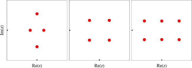
Figure 5. The root structures of Wronskian-Hermite polynomials W$\Lambda$(z) in the complex z-plane, where index vectors $\Lambda$ are given by (1, 4), (2, 3) and (2, 3, 4), from left to right, respectively. In both panels, $-4\leqslant \mathrm{Re}(z),\mathrm{Im}(z)\leqslant 4$. |
In fact, it turns out that the root structure of W$\Lambda$(z) is closely related to large-time patterns of rogue curves. Now, we analytically predict the asymptotic wave dynamics of rogue waves in the DSI equation at large times. In our discussions, we first restrict p = 1 in DSI's rogue wave solutions (2 )-(3 ). The case when p ≠ 1 will be discussed separately.
For the general index vector $\Lambda$ ≠ (1, 3, 5, …, 2N - 1), we will show that when time is large, the asymptotic wave dynamics of DSI rogue curves and locations of these lump-shaped waves in the (x, y) plane would be predicted by the root structure of W$\Lambda$(z). Our main results are concluded as the following theorem.
Suppose the index vector $\Lambda$ ≠ (1, 3, 5, …, 2N - 1). Then, for large time |t| » 1, when (x, y) is in the O(1) neighborhood of the location (x0, y0), the solution |A$\Lambda$(x, y, t)| would asymptotically separates into $({N}_{w}-\frac{1}{2}{N}_{R}-\frac{1}{2}{N}_{I})$ line solitons A1(x, y, t), whose expression is
$\begin{eqnarray}{A}_{1}(x,y,t)=\sqrt{2}\left[\frac{({F}_{1}(x,y,t)+1)({F}_{1}^{* }(x,y,t)-1)+\frac{1}{4}}{| {F}_{1}(x,y,t){| }^{2}+\frac{1}{4}}\right],\end{eqnarray}$
where F1(x, y, t) is defined as $\begin{eqnarray}{F}_{1}(x,y,t)=y-{y}_{0}-\frac{\sqrt{2}}{2}{z}_{0}\left(\sqrt{x}-\sqrt{{x}_{0}}\right),\end{eqnarray}$
or equivalently, $\begin{eqnarray}{F}_{1}(x,y,t)=y-{z}_{0}\sqrt{\frac{x}{2}}-2{\rm{i}}t,\end{eqnarray}$
and the leading-order positions (x0, y0) are predicted by $\begin{eqnarray}({y}_{0}-2it)={z}_{0}{\left(\frac{1}{2}{x}_{0}\right)}^{\frac{1}{2}},\end{eqnarray}$
where z0 represents each of the Nw nonzero simple roots of W$\Lambda$(z), and Nw is given by equation ( $\begin{eqnarray}{A}_{{\rm{\Lambda }}}(x,y,t)={A}_{1}(x,y,t)+O\left(| t{| }^{-2}\right),\,\,\,| t| \gg 1.\end{eqnarray}$
When (x, y) is not in the neighborhood of each line soliton, the solution |A$\Lambda$(x, y, t)| asymptotically approach the constant backgrounds $\sqrt{2}$ as |t| → ∞. The demonstration of this theorem will be presented in a later section.On Theorem 1, we have the following remark: equation (21 ) defines a corresponding relation between the predicted location (x0, y0) at large times and nonzero simple root z0 of the Wronskian-Hermite polynomials. Through simple analysis, we could see from equations (18 )-(20 ) that this correspondence is a nonlinear mapping. For each (x0, y0) location in the (x, y)-spatial plane, it matches a unique z0 on the specific region of the complex z-plane. This correspondence relation between the sign of (x0, y0) and the sign of z0 is given in tables 1 and 2 for large positive and negative time values, separately.
Table 1. The correspondence relation for t > 0. |
| Sign of (x0, y0) in the (x, y) plane | Sign of z0 in the complex plane |
|---|---|
| x0 > 0, y0 > 0 | ${\rm{Re}}({z}_{0})\gt 0,\,{\rm{Im}}({z}_{0})\lt 0$ |
| x0 > 0, y0 < 0 | ${\rm{Re}}({z}_{0})\lt 0,\,{\rm{Im}}({z}_{0})\lt 0$ |
| x0 < 0, y0 > 0 | ${\rm{Re}}({z}_{0})\lt 0,\,{\rm{Im}}({z}_{0})\lt 0$ |
| x0 < 0, y0 < 0 | $\mathrm{Re}({z}_{0})\lt 0,\,\mathrm{Im}({z}_{0})\gt 0$ |
Table 2. The correspondence relation for t < 0. |
| Sign of (x0, y0) in the (x, y) plane | Sign of z0 in the complex plane |
|---|---|
| x0 > 0, y0 > 0 | ${\rm{Re}}({z}_{0})\gt 0,\,{\rm{Im}}({z}_{0})\gt 0$ |
| x0 > 0, y0 < 0 | ${\rm{Re}}({z}_{0})\lt 0,\,{\rm{Im}}({z}_{0})\gt 0$ |
| x0 < 0, y0 > 0 | ${\rm{Re}}({z}_{0})\gt 0,\,{\rm{Im}}({z}_{0})\lt 0$ |
| x0 < 0, y0 < 0 | ${\rm{Re}}({z}_{0})\gt 0,\,{\rm{Im}}({z}_{0})\gt 0$ |
In addition, if the polynomial W$\Lambda$(z) has zero root, due to equation (21 ), then it is found that the zero root will not induce any wave patterns at large times.
4. Comparison between analytical predictions and true solutions
Now, we compare analytical predictions with true solutions shown in figures 2, 3 and 4 at large times. For the first parameter choices (12 ) where $\Lambda$ = (1, 4), the corresponding root structure of W$\Lambda$(z) has been illustrated in the left panel of figure 5. It is seen that this W$\Lambda$(z) admits four simple nonzero roots, including two real roots and two imaginary roots, which form a rhombus shape. Utilizing this root structure, we can derive predicted wave patterns similar to true solutions shown in figure 2 at large times. This predicted pattern consists of two line solitons. To better compare the change in the shape of waves to true ones, we choose one of these two individual line solitons, which corresponds to the one marked by a white arrow in figure 2. Then, at three time values of t = 10, 20 and 30, this A1(x, y, t) prediction is plotted in figure 6. When comparing this to figure 2, we visually see that they closely match each other in all aspects.
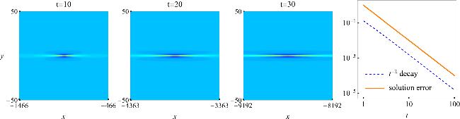
Figure 6. The leading-order analytical prediction of the asymptotic line soliton marked by a white arrow in figure 2, at three time values of t = 10, 20 and 30. The (x, y) intervals here are the same as those in figure 2 for comparison. The rightmost panel shows the error of the leading-order prediction versus time for this line soliton (the theoretical decay rate of t-2 is also plotted for comparison). |
Furthermore, in order to verify the decay rate of relative errors on positions of these line solitons, we quantitatively compare predicted and true solutions at various time values. For this line soliton, we numerically determine at each large time t the relative error of prediction for its position, which is defined as 21 ).
$\begin{eqnarray}\,\rm{relative error}\,=\,\frac{\sqrt{{({x}_{0,\mathrm{true}}-{x}_{0})}^{2}+{({y}_{0,\mathrm{true}}-{y}_{0})}^{2}}}{\sqrt{{({x}_{0,\mathrm{true}})}^{2}+{({y}_{0,\mathrm{true}})}^{2}}},\end{eqnarray}$
where (x0,true, y0,true) is the true peak location of the line soliton, and (x0, y0) is its leading-order prediction from equation (Then, we plot in the rightmost panel of figure 6 the relative error of prediction versus time t for that line soliton marked by a white arrow in the upper rightmost panel of figure 2. The actual error graph in the rightmost panel shows that its decay rate is indeed O(t-2), confirming our theoretical prediction (22 ).
Next, we compare the true solution in figure 3 to our prediction for the second parameter choices (13 ). In this case, $\Lambda$ = (2, 3), and the corresponding root structure of W$\Lambda$(z) has been plotted in the middle panel of figure 5. It was seen that this W$\Lambda$(z) admits four simple nonzero complex roots z0 which form a square pattern. Using this root structure, we can obtain the predicted wave patterns at large times.
This predicted pattern consists of four line soliton solutions. To better compare their wave dynamics to true ones at large times, we choose one of these four individual line solitons, which corresponds to the one marked by a white arrow in the upper rightmost panel of figure 3. Then, at three time values of t = 15, 30 and 60, we plot this A1(x, y, t) prediction in figure 7. Comparing this to figure 3, we could observe a strong visual agreement between the predicted and true solutions.
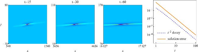
Figure 7. Leading-order analytical prediction of the asymptotic line soliton marked by a white arrow in figure 3, at three time values of t = 15, 30 and 60. The (x, y) intervals here are the same as those in figure 3 for comparison. The rightmost panel shows the error of the leading-order prediction versus time for this line soliton (the theoretical decay rate of t-2 is also plotted for comparison). |
We have also numerically verified O(t-2) error decay rate of our prediction (22 ) for the line soliton associated with a nonzero root of W$\Lambda$(z). To be specific, we plot in the rightmost panel of figure 7 the relative error of prediction versus time for the line soliton marked by a white arrow in the upper rightmost panel of figure 3. The actual error graph in the rightmost panel shows that its decay rate is indeed O(t-2), confirming our theory.
Last, we compare the true solution in figure 4 to our prediction for the second parameter choices (14 ). In this case, $\Lambda$ = (2, 3, 4), and the corresponding root structure of W$\Lambda$(z) has been plotted in the right panel of figure 5. It was seen that this W$\Lambda$(z) admits six simple nonzero roots z0 which form a rectangular pattern. Using this root structure, we can obtain the predicted wave patterns at large times. This predicted pattern consists of five line soliton solutions, as theorem 1 predicts. Then, at two time values of t = -15 and 15, we plot this A1(x, y, t) prediction in figure 8. Comparing this to figure 4, visually, we could observe an excellent agreement between the true and predicted wave patterns. In addition, similar to what we did for the previous two examples in figures 6 and 7, we have also quantitatively measured the error of analytical predictions versus time. It is confirmed that the error does decay in proportion to t-2. The corresponding error-decay graphs are omitted here for brevity. Thus, the numerical verification of theorem 1 are completed.
Figure 8. The leading-order analytical prediction of a DSI rogue curve (|A$\Lambda$(x, y, t)|) for parameter choices of ( |
At the end of this section, we would like to briefly discuss potential physical applications of these rogue curve patterns in real-world nonlinear wave propagation systems. It is well-known that rogue wave patterns predicted by the NLS equation and the Manakov system have been observed in different physical experiments including optical fibers, water tanks, Bose-Einstein condensates and plasma physics. The perfect match between analytical solutions and experimental observations has been revealed [25]. However, for those rogue curve solutions in DSI equation, as far as we know, relevant laboratory experiments have not been reported. It is anticipated that our analytical predictions from theorem 1 may facilitate possible observations or experiment setup on these rogue curve patterns in the context of water waves. These large-time wave patterns are expected to be important in understanding and forecasting natural rogue events in a variety of multi-component resonant interaction processes.
5. Proof of theorem 1
In the following, we prove analytical predictions in theorem 1. First of all, we rewrite the determinant Γk in equation (5 ) as a broader (N + nN + 1) × (N + nN + 1) determinant 6 )-(9 ). Then we have 24 ) can be rewritten as
$\begin{eqnarray}{\tau }_{k}=\left|\begin{array}{cc}{{\boldsymbol{O}}}_{N\times N} & {{\rm{\Phi }}}_{N\times ({n}_{N}+1)}\\ -{{\rm{\Psi }}}_{({n}_{N}+1)\times N} & {{\boldsymbol{I}}}_{({n}_{N}+1)\times ({n}_{N}+1)}\end{array}\right|,\end{eqnarray}$
where $\begin{eqnarray}{{\rm{\Phi }}}_{i,j}={2}^{-(j-1)}{S}_{{n}_{i}+1-j}\left({{\boldsymbol{x}}}^{+}(k)+(j-1){\boldsymbol{s}}\right),\end{eqnarray}$
$\begin{eqnarray}{{\rm{\Psi }}}_{i,j}={2}^{-(i-1)}{S}_{{n}_{j}+1-i}\left({{\boldsymbol{x}}}^{-}(k)+(i-1){\boldsymbol{s}}\right),\end{eqnarray}$
where vectors x±(k) and s are as defined in equations ( $\begin{eqnarray}{x}_{1}^{\pm }(k)=y\mp 2{\rm{i}}t\pm k,\end{eqnarray}$
$\begin{eqnarray}{x}_{2}^{+}=\frac{1}{2}x+{a}_{2},\,{x}_{2}^{-}={({x}_{2}^{+})}^{* },\end{eqnarray}$
and so on. Using Laplace expansion, determinant ( $\begin{eqnarray}\begin{array}{rcl}{\tau }_{k} & = & \displaystyle \sum _{0\leqslant {\nu }_{1}\lt {\nu }_{2}\lt \cdots \lt {\nu }_{N}\leqslant {n}_{N}}\mathop{\det }\limits_{1\leqslant i,j\leqslant N}\left[\frac{1}{{2}^{{\nu }_{j}}}{S}_{{n}_{i}-{\nu }_{j}}\left({{\boldsymbol{x}}}^{+}(k)+{\nu }_{j}{\boldsymbol{s}}\right)\right]\\ & & \times \mathop{\det }\limits_{1\leqslant i,j\leqslant N}\left[\frac{1}{{2}^{{\nu }_{j}}}{S}_{{n}_{i}-{\nu }_{j}}\left({{\boldsymbol{x}}}^{-}(k)+{\nu }_{j}{\boldsymbol{s}}\right)\right].\end{array}\end{eqnarray}$
Now, for |t| » 1, suppose x = O(t2), y = O(t), with internal parameters satisfying the constraint ak = o(|t|k) in the general high-order rational solutions. In this case, we have the following asymptotic: 15 ), and
$\begin{eqnarray*}\begin{array}{rcl}{S}_{n}\left({{\boldsymbol{x}}}^{+}+\nu {\boldsymbol{s}}+{\boldsymbol{a}}\right) & \sim & {S}_{n}\left(y-2it,\frac{1}{2}x,0,\cdots \,\right)\\ & = & {\left(\frac{1}{2}x\right)}^{\frac{n}{2}}{S}_{n}\left(z,1,0,\cdots \,\right)\\ & = & {\left(\frac{1}{2}x\right)}^{\frac{n}{2}}{q}_{n}(z),\end{array}\end{eqnarray*}$
where qn(z) is defined in equation ( $\begin{eqnarray}z={\left(\frac{1}{2}x\right)}^{-\frac{1}{2}}\left(y-2it\right).\end{eqnarray}$
Similarly, we also have
$\begin{eqnarray*}{S}_{n}\left({{\boldsymbol{x}}}^{-}+\nu {\boldsymbol{s}}+{\boldsymbol{a}}\right)\sim {\left[{\left(\frac{1}{2}x\right)}^{\frac{n}{2}}\right]}^{* }{q}_{n}^{* }(z).\end{eqnarray*}$
Therefore, choosing the index νj = j - 1, we can readily show that the highest power of t term in Γk is 16 ). It can be shown through equation (2 ) that solution A$\Lambda$(x, y, t) approaches constant background $\sqrt{2}$ as |t| → ∞, except at or near (x, y) locations (x0, y0), where
$\begin{eqnarray}{\tau }_{k}\sim {2}^{-N(N-1)}{\left|\frac{1}{2}x\right|}^{\rho }| {W}_{{\rm{\Lambda }}}(z){| }^{2},\,\,\,| t| \gg 1,\end{eqnarray}$
where ρ is defined in equation ( $\begin{eqnarray}\left({y}_{0}-2it\right)={z}_{0}{\left(\frac{1}{2}{x}_{0}\right)}^{\frac{1}{2}},\end{eqnarray}$
z0 represents any complex root of the Wronskian-Hermite polynomial W$\Lambda$(z).Next, we demonstrate large time asymptotic behavior of the solution in the O(1) neighborhood of (x0, y0). For this purpose, we need a more refined asymptotic for ${S}_{n}\left({{\boldsymbol{x}}}^{+}(k)+\nu \,{\boldsymbol{s}}\right)$ 29 ) for Γk near the location. There are two sources of contributions. For the first index choice (ν1, ν2, …, νN) = (0, 1, …, N - 1), we get 19 ) in theorem 1.
$\begin{eqnarray*}\begin{array}{l}{S}_{n}\left({{\boldsymbol{x}}}^{+}(k)+\nu {\boldsymbol{s}}\right)={S}_{n}\left(y-2{\rm{i}}t+k,\frac{x}{2}+\nu \,{s}_{2}+{a}_{2},\cdots \,\right)\\ \quad =\,{\left(\frac{1}{2}x\right)}^{\frac{n}{2}}{S}_{n}\left(\hat{z},1,0,\cdots \,\right)\left[1+O(| t{| }^{-2})\right],\end{array}\end{eqnarray*}$
where $\hat{z}=(y-2{\rm{i}}t+k){\left(\frac{1}{2}x\right)}^{-\frac{1}{2}}$. Now, we collect the dominant contributions in the Laplace expansion ( $\begin{eqnarray*}\begin{array}{l}\mathop{\det }\limits_{1\leqslant i,j\leqslant N}\left[\frac{1}{{2}^{j-1}}{S}_{{n}_{i}-j+1}({{\boldsymbol{x}}}^{+}(k)+\nu {\boldsymbol{s}})\right]\\ =\,{2}^{-\frac{N(N-1)}{2}}{\left(\frac{1}{2}x\right)}^{\frac{\rho }{2}}{W}_{{\rm{\Lambda }}}(\hat{z})\left[1+O(| t{| }^{-2})\right]\\ =\,{2}^{-\frac{N(N-1)}{2}}{\left(\frac{1}{2}x\right)}^{\frac{\rho }{2}}\left[{W}_{{\rm{\Lambda }}}^{{\prime} }({z}_{0})(\hat{z}-{z}_{0})+\cdots \,\right]\left[1+O(| t{| }^{-2})\right],\\ =\,{2}^{-\frac{N(N-1)}{2}}{\left(\frac{1}{2}x\right)}^{\frac{\rho -1}{2}}\left[{W}_{{\rm{\Lambda }}}^{{\prime} }({z}_{0})\left({F}_{1}(x,y,t)+k\right)+O(| t{| }^{-1})\right],\end{array}\end{eqnarray*}$
where the expression of F1(x, y, t) has been given by equation (Similarly, we get
$\begin{eqnarray*}\begin{array}{l}\mathop{\det }\limits_{1\leqslant i,j\leqslant N}\left[\frac{1}{{2}^{j-1}}{S}_{{n}_{i}-j+1}({{\boldsymbol{x}}}^{-}(k)+\nu {\boldsymbol{s}})\right]\\ \quad ={2}^{-\frac{N(N-1)}{2}}{\left[{\left(\frac{1}{2}x\right)}^{\frac{\rho -1}{2}}\right]}^{* }\\ \quad \left[\times ,[,{W}_{{\rm{\Lambda }}}^{{\prime} }({z}_{0}^{* })\left({F}_{1}^{* }(x,y,t)-k\right)+O(| t{| }^{-1})\right].\end{array}\end{eqnarray*}$
Therefore, the contribution to the Laplace expansion (29 ) from the νj = j - 1 indices is
$\begin{eqnarray*}\begin{array}{rcl}{\tau }_{k} & = & {2}^{-N(N-1)}{\left|\frac{1}{2}x\right|}^{\rho -1}\\ & & \times | {W}_{{\rm{\Lambda }}}^{{\prime} }({z}_{0}){| }^{2}\left({F}_{1}(x,y,t)+k\right)\\ & & \times \left({F}_{1}^{* }(x,y,t)-k\right)[1+O(| t{| }^{-1})].\end{array}\end{eqnarray*}$
For the other index choice (ν1, ν2, …, νN) =(0, 1, N - 2, …, N), we get 2 ), we get the asymptotic prediction for solution A(x, y, t) as
$\begin{eqnarray*}\begin{array}{rcl}{\tau }_{k} & = & {2}^{-N(N-1)-2}{\left|\frac{1}{2}x\right|}^{\rho -1}\\ & & \times | {W}_{{\rm{\Lambda }}}^{{\prime} }({z}_{0}){| }^{2}[1+O(| t{| }^{-1})].\end{array}\end{eqnarray*}$
Based on these two dominant contributions, we have $\begin{eqnarray*}\begin{array}{rcl}{\tau }_{k} & = & {2}^{-N(N-1)}{\left|\frac{1}{2}x\right|}^{\rho -1}\\ & & \times | {W}_{{\rm{\Lambda }}}^{{\prime} }({z}_{0}){| }^{2}\left[\left({F}_{1}(x,y,t)+k\right)\left({F}_{1}^{* }(x,y,t)-k\right)+\frac{1}{4}\right]\\ & & \times [1+O(| t{| }^{-1})].\end{array}\end{eqnarray*}$
Substituting this asymptotics of Γk into equation ( $\begin{eqnarray*}\begin{array}{rcl}{A}_{{\rm{\Lambda }}}(x,y,t) & = & \sqrt{2}\left[1-\frac{2{\rm{i}}\Im ({F}_{1}(x,y,t))+1}{| {F}_{1}(x,y,t){| }^{2}+\frac{1}{4}}\right]\\ & & \times [1+O(| t{| }^{-1})],\end{array}\end{eqnarray*}$
where $\mathfrak{I}$ represent the imaginary parts of a complex number. This concludes the proof of theorem 1.6. Large-time asymptotic predictions for p ≠ 1
In theorem 1, we have set p = 1. In this section, we discuss large-time asymptotic for rogue curves when p ≠ 1 and real. In this more general case, from equations (6 )-(9 ), we have 15 ), and 29 ), we can get 2 ) that solution A$\Lambda$(x, y, t) approaches constant background $\sqrt{2}$ as |t| → ∞, except at or near (x, y) locations (x0, y0), where 35 ) can be seen as the counterpart of the previous one given by equation (32 ) for the p = 1 case. Moreover, the leading-order predicted location (x0, y0) for p ≠ 1 is related to that for p = 1 through a linear transformation
$\begin{eqnarray*}\begin{array}{rcl}{x}_{1}^{+}(k) & = & {c}_{11}x+{c}_{12}y-{c}_{13}{\rm{i}}t+k,\\ {x}_{1}^{-}(k) & = & {\left[{x}_{1}^{+}(-k)\right]}^{\ast },\\ {x}_{2}^{+} & = & {c}_{21}x+{c}_{22}y-{c}_{23}{\rm{i}}t+{a}_{2},\\ {x}_{2}^{-} & = & {\left({x}_{2}^{+}\right)}^{\ast },\end{array}\end{eqnarray*}$
and so on, where the p-dependent coefficients are given as $\begin{eqnarray*}\begin{array}{rcl}{c}_{11} & = & \frac{p-{p}^{-1}}{2},\quad {c}_{12}=\frac{p+{p}^{-1}}{2},\\ {c}_{13} & = & {p}^{2}+{p}^{-2}\gt 0,\\ {c}_{21} & = & \frac{p+{p}^{-1}}{4},\quad {c}_{22}=\frac{p-{p}^{-1}}{4},\\ {c}_{23} & = & {p}^{2}-{p}^{-2}.\end{array}\end{eqnarray*}$
Then, for |t| » 1, c11x + c12y = O(t), c21x + c22y = O(t2), with internal parameters satisfying the constraint ak = o(|t|k) in the general high-order rational solutions, we have $\begin{eqnarray*}\begin{array}{l}{S}_{n}\left({{\boldsymbol{x}}}^{+}+\nu {\boldsymbol{s}}+{\boldsymbol{a}}\right)\sim {S}_{n}({c}_{11}x\\ \,+{c}_{12}y-{c}_{13}{\rm{i}}t,{c}_{21}x+{c}_{22}y-{c}_{23}{\rm{i}}t,0,\cdots \,)\\ =\,{\left({c}_{21}x+{c}_{22}y\right)}^{\frac{n}{2}}{S}_{n}(z,1,0,\cdots \,)\\ =\,{\left({c}_{21}x+{c}_{22}y\right)}^{\frac{n}{2}}{q}_{n}(z),\end{array}\end{eqnarray*}$
where qn(z) is defined in equation ( $\begin{eqnarray}z={({c}_{21}x+{c}_{22}y)}^{-\frac{1}{2}}\left({c}_{11}x+{c}_{12}y-{c}_{13}{\rm{i}}t\right).\end{eqnarray}$
Similarly, we could also show that $\begin{eqnarray*}{S}_{n}\left({{\boldsymbol{x}}}^{-}+\nu {\boldsymbol{s}}+{\boldsymbol{a}}\right)\sim {\left[{\left({c}_{21}x+{c}_{22}y\right)}^{\frac{n}{2}}\right]}^{* }{q}_{n}^{* }(z).\end{eqnarray*}$
Therefore, from the Laplace expansion ( $\begin{eqnarray}{\tau }_{k}\sim {2}^{-N(N-1)}{\left|{c}_{21}x+{c}_{22}y\right|}^{\rho }| {W}_{{\rm{\Lambda }}}(z){| }^{2},\,\,\,| t| \gg 1.\end{eqnarray}$
It can be shown through equation ( $\begin{eqnarray}{c}_{11}{x}_{0}+{c}_{12}{y}_{0}-{c}_{13}{\rm{i}}t={z}_{0}{\left({c}_{21}{x}_{0}+{c}_{22}{y}_{0}\right)}^{\frac{1}{2}},\end{eqnarray}$
z0 is a complex root of the Wronskian-Hermite polynomial W$\Lambda$(z). Equation ( $\begin{eqnarray*}{\left.\left(\begin{array}{c}{x}_{0}\\ {y}_{0}\end{array}\right)\right|}_{p=1}=\left(\frac{2}{{c}_{13}}\right)\left(\begin{array}{cc}\frac{4{c}_{21}}{{c}_{13}} & \frac{4{c}_{22}}{{c}_{13}}\\ {c}_{11} & {c}_{12}\end{array}\right){\left.\left(\begin{array}{c}{x}_{0}\\ {y}_{0}\end{array}\right)\right|}_{p\ne 1}.\end{eqnarray*}$
Next, we demonstrate large time asymptotic prediction for the solution when (x, y) is in the O(1) neighborhood of location (x0, y0). Similar to what we have done earlier for p = 1 case, the asymptotic prediction of the solution A$\Lambda$(x, y, t) is found to be
$\begin{eqnarray*}\begin{array}{rcl}{A}_{{\rm{\Lambda }}}(x,y,t) & = & \sqrt{2}\left[1-\frac{2{\rm{i}}\Im ({G}_{1}(x,y,t))+1}{{\left|{G}_{1}(x,y,t)\right|}^{2}+\frac{1}{4}}\right]\\ & & \times [1+O(| t{| }^{-1})],\end{array}\end{eqnarray*}$
where $\begin{eqnarray}\begin{array}{rcl}{G}_{1}(x,y,t) & = & {c}_{11}x+{c}_{12}y\\ & & -{z}_{0}\sqrt{{c}_{21}x+{c}_{22}y}-{c}_{13}{\rm{i}}t.\end{array}\end{eqnarray}$
7. Conclusions and discussions
In this article, we have analytically and numerically studied large time asymptotic wave dynamics of rogue curves in the DSI equation. We have demonstrated that, when time in bilinear expressions of the DSI rogue curves is large, a certain number of lump-shaped waves would appear on the uniform background, exhibiting various wave patterns. Performing large-time asymptotic analysis, we have discovered that such wave patterns as well as the numbers of lump-shaped waves can be analytically determined by structure of nonzero roots of the Wronskian-Hermite polynomials. We have further discovered that, as time increases, these individual lump-shaped waves asymptotically become a line soliton on the constant background. Our asymptotic predictions are compared to true solutions quantitatively, and excellent agreement has been obtained.
We have also noticed that long-time asymptotic wave dynamics of the higher-order lumps in the DSI equation was analytically studied in [29], and it was found that wave patterns for those lumps were determined by roots of special Wronskian type polynomials. By comparing the results of their study to ours, the main distinguishing feature here is the changes of state in rogue curves, where a lump-shaped wave asymptotically turns into a line soliton when time increases. On the other hand, when comparing these results to large-time wave patterns of KPI lumps in [30], where each fundamental lump in the solution at large time relates to a simple root of the underlying Wronskian-Hermite polynomials, and this connection is a one-to-one correspondence. However, in our case, it is found that the relation between nonzero simple root of the underlying Wronskian-Hermite polynomial and the individual line soliton in rogue curves at large time is no longer a linear one-to-one mapping. These differences mentioned above reflect the diversity and complexity of nonlinear wave patterns. The deep connections between wave propagation phenomena and root structures of certain polynomials are expected to be discovered again in other physically important wave systems.
The robustness simulations of rogue waves has been investigated before in the NLS equation and some other one-dimensional integrable systems [25]. It was found that under weak perturbations, the underlying rogue waves are still observable. Similarly, for these two-dimensional rogue curves in the DSI equation, it would be interesting to see whether they could survive weak perturbations, especially at large times. Another interesting question that merits future studies is whether these rogue curves and their large-time wave patterns would also appear in other (2+1)-dimensional integrable systems, such as the (2+1)-dimensional three-wave resonant interaction system [31], or the two-dimensional multi-component long-wave-short-wave interaction system [32], for instance.