Welcome to visit Communications in Theoretical Physics,
Quantum Physics and Quantum Information

Exact analytical results for a two-level system driven by a pulse with Lorentzian frequency and sub-Lorentzian amplitude modulations

  • Qiong-Tao Xie
Expand
  • College of Physics and Electronic Engineering, Key Laboratory of Laser Technology and Optoelectronic Functional Materials of Hainan Province, Hainan Normal University, Haikou 571158, China

Received date: 2025-06-27

  Revised date: 2025-10-12

  Accepted date: 2025-10-13

  Online published: 2025-11-14

Copyright

© 2025 Institute of Theoretical Physics CAS, Chinese Physical Society and IOP Publishing. All rights, including for text and data mining, AI training, and similar technologies, are reserved.
This article is available under the terms of the IOP-Standard License.

Abstract

We investigate the dynamics of a two-level quantum system driven by a laser pulse characterized by Lorentzian frequency and sub-Lorentzian amplitude modulations. Complete analytical solutions, expressed via confluent Heun functions, are derived. Our analysis reveals that explicit exact analytical solutions exist under infinite sets of specific parameter conditions. The effects of modulation parameters and initial conditions on the final transition probabilities are examined analytically and numerically. Furthermore, the method is demonstrated to be directly applicable to two closely related models with Lorentzian pulses.

Cite this article

Qiong-Tao Xie . Exact analytical results for a two-level system driven by a pulse with Lorentzian frequency and sub-Lorentzian amplitude modulations[J]. Communications in Theoretical Physics, 2026 , 78(3) : 035101 . DOI: 10.1088/1572-9494/ae120a

1. Introduction

Coherent laser fields provide an efficient tool for controlling the dynamical behavior of quantum systems [1, 2]. Due to its simplicity, the laser-driven two-level system has become a prototypical model for demonstrating quantum control principles [3]. When the laser fields are treated classically, time-dependent two-level models (TLMs) are commonly employed. As exact analytical solutions are fundamentally important for understanding quantum control physics, the search for exactly solvable time-dependent (ESTD) TLMs has attracted extensive research interest over several decades.
The first nontrivial ESTD TLM was proposed by Landau and Zener [4, 5], where the level bias changes linearly in time. Subsequently, numerous ESTD TLMs have been discovered, including Rosen-Zener [6], Nikitin [7], Demkov [8], Demkov-Kunike [9], Bambini-Berman [10], Bambini-Lindberg [11], Hioe [12], Robinson [13], Hioe-Carroll [14], Carroll-Hioe [15, 16], Allen-Eberly [17], Ishkhanyan [18, 19], and Vitanov [20, 21] models. This list is non-exhaustive. Despite their apparent simplicity, such models find extensive applications in atomic/molecular physics, quantum optics, and quantum information.
There are two primary approaches for constructing ESTD TLMs. The first utilizes specific laser amplitude and frequency modulations such that, through appropriate variable transformation, the Schrödinger equation reduces to well-studied second-order differential equation. While hypergeometric and confluent hypergeometric equations have predominated in earlier studies, recent extensions employ the Heun equation and its confluent forms [22-31]. The second approach employs reverse-engineering algorithms to generate unlimited exact solutions [32-36]. Except in limited cases, these solutions typically require complex laser-field modulations that remain experimentally challenging [37, 38]. Moreover, for more complex field excitations, various numerical algorithms have been developed and applied, including Yee's finite-difference time-domain discretization method [39, 40] and the predictor-corrector method [41-43].
The Lorentzian pulse is commonly utilized in current experiments [37]. While the exact analytical solution for standard Lorentzian TLMs remains under investigation, a double Lorentzian TLM has recently been proposed [26, 31]. In this system, a two-level quantum system is subjected to a laser pulse featuring both Lorentzian-modulated frequency and Lorentzian-modulated amplitude. Analytical solutions for the double Lorentzian TLM can be expressed using confluent Heun functions (CHFs). But these solutions are incomplete. Furthermore, from the termination conditions for CHFs, explicit solutions have only been obtained for certain specific parameter conditions. Finding exact solutions for generic system parameters, outside these restrictive termination conditions, remains elusive.
Here we introduce a novel class of time-dependent TLMs featuring Lorentzian frequency and sub-Lorentzian amplitude modulations. For simplicity, we term this model the mixed Lorentzian TLM. We demonstrate that the corresponding Schrödinger equation is exactly reducible to the confluent Heun equation (CHE) through an appropriate variable transformation. An analytical method is developed to express the complete analytical solutions in terms of CHFs. Furthermore, infinite sets of explicit closed-form solutions emerge under parameter constraints derived from CHF termination conditions. Using these exact solutions, we systematically investigate the parametric dependence of final transition probabilities on system properties and initial conditions. In particular, we derive an exact analytical expression for transition probabilities when parameters deviate from termination conditions, under which the population admits a simple functional form. This formalism directly applies to broader cases, including the double-Lorentzian TLM and a single Lorentzian TLM with Lorentzian frequency modulation but constant amplitude.

2. Model and analytical solutions

We consider a two-level quantum system driven by a nonresonant laser field, described by the time-dependent Hamiltonian (ħ = 1)
$\begin{eqnarray}H=\frac{f(t)}{2}{\sigma }_{z}+\frac{\nu (t)}{2}{\sigma }_{x},\end{eqnarray}$
where σx,z are the usual Pauli matrices, f(t) represents the detuning from resonance, and ν(t) describes the coupling between levels, corresponding to the temporal laser profile. The probability amplitudes a1(t) and a2(t) obey the coupled equations
$\begin{eqnarray}{\rm{i}}\displaystyle \frac{{\rm{d}}{a}_{1}}{{\rm{d}}t}=\displaystyle \frac{\nu (t)}{2}{a}_{2}+\displaystyle \frac{f(t)}{2}{a}_{1},\end{eqnarray}$
$\begin{eqnarray}{\rm{i}}\displaystyle \frac{{\rm{d}}{a}_{2}}{{\rm{d}}t}=\displaystyle \frac{\nu (t)}{2}{a}_{1}-\displaystyle \frac{f(t)}{2}{a}_{2}.\end{eqnarray}$
Elimination of a2(t) and a1(t) yields second-order differential equations
$\begin{eqnarray}\displaystyle \frac{{{\rm{d}}}^{2}{a}_{1}}{{\rm{d}}{t}^{2}}-\displaystyle \frac{\dot{\nu }}{\nu }\displaystyle \frac{{\rm{d}}{a}_{1}}{{\rm{d}}t}+\left(\displaystyle \frac{{f}^{2}}{4}+\displaystyle \frac{{\nu }^{2}}{4}+{\rm{i}}\displaystyle \frac{\dot{f}}{2}-{\rm{i}}\displaystyle \frac{f}{2}\displaystyle \frac{\dot{\nu }}{\nu }\right){a}_{1}=0,\end{eqnarray}$
$\begin{eqnarray}\displaystyle \frac{{{\rm{d}}}^{2}{a}_{2}}{{\rm{d}}{t}^{2}}-\displaystyle \frac{\dot{\nu }}{\nu }\displaystyle \frac{{\rm{d}}{a}_{2}}{{\rm{d}}t}+\left(\displaystyle \frac{{f}^{2}}{4}+\displaystyle \frac{{\nu }^{2}}{4}-{\rm{i}}\displaystyle \frac{\dot{f}}{2}+{\rm{i}}\displaystyle \frac{f}{2}\displaystyle \frac{\dot{\nu }}{\nu }\right){a}_{2}=0,\end{eqnarray}$
where dots denote time derivatives, $\dot{f}={\rm{d}}f/{\rm{d}}t$ and $\dot{\nu }={\rm{d}}\nu /{\rm{d}}t$. Equations (4) and (5) possess conjugate solution pairs: if Φ(t) solves equation (4), then Φ*(t) solves equation (5). This symmetry simplifies subsequent analysis. Once a1(t) is determined, a2(t) follows from equation (2).
Prior works [26, 31] investigated the double Lorentzian temporal laser model with
$\begin{eqnarray}f(t)={f}_{0}+\frac{{f}_{1}}{1+{g}^{2}{t}^{2}},\nu (t)=\frac{{\nu }_{1}}{1+{g}^{2}{t}^{2}},\end{eqnarray}$
where f0 is constant detuning, f1/(1 + g2t2) denotes the Lorentzian frequency modulation, and ν1/(1 + g2t2) describes the Lorentzian amplitude modulation. Here the parameter g is related to the width scale Γ, g = π/Γ. This double Lorentzian TLM generalizes the standard Lorentzian TLM (where f1 = 0) to include both amplitude and frequency modulations.
Here we propose a mixed Lorentzian TLM with Lorentzian frequency and sub-Lorentzian amplitude modulations
$\begin{eqnarray}f(t)={f}_{0}+\frac{{f}_{1}}{1+{g}^{2}{t}^{2}},\nu (t)=\frac{{\nu }_{1}}{\sqrt{1+{g}^{2}{t}^{2}}}.\end{eqnarray}$
Typical profiles of this frequency and amplitude modulations are shown in figure 1 with g = 1, f0/g = 0.5, f1/g = 0.2, and ν1/g = 0.6. Furthermore, in the case of gt « 1, we can approximate the detuning f(t) by Taylor series expansion
$\begin{eqnarray}f(t)\approx {f}_{0}+{f}_{1}-{f}_{1}{(gt)}^{2},\end{eqnarray}$
revealing that the laser pulse frequency varies quadratically with time [44].
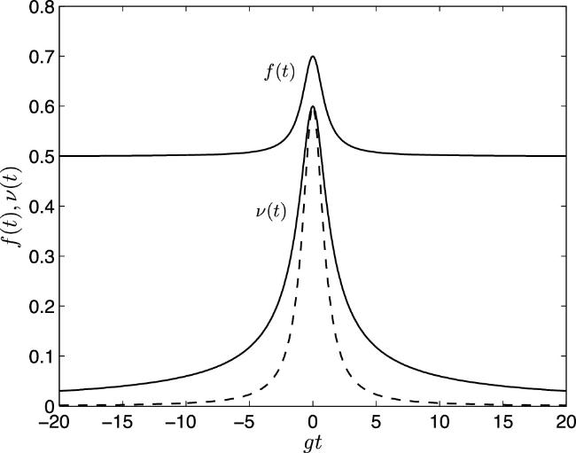
Figure 1. Modulation profiles for the frequency and amplitude described in equations (6) and (7) as a function of gt. Here f0/g = 0.5, f1/g = 0.2, ν1/g = 0.6, and g = 1. The solid lines show the modulations from equation (7), while the dashed line corresponds to equation (6).
To solve the system equation (4) under modulation equation (7), we apply the transformations
$\begin{eqnarray}\begin{array}{l}\,z=\displaystyle \frac{1}{2}(1-{\rm{i}}gt),\\ {a}_{1}(z)={{\rm{e}}}^{-{\rm{i}}{\lambda }_{1}gt/2}{(1-{\rm{i}}gt)}^{{\lambda }_{2}}{(1+{\rm{i}}gt)}^{{\lambda }_{3}}\phi (z),\end{array}\end{eqnarray}$
with parameters given by (see Appendix A)
$\begin{eqnarray}{\lambda }_{1}=\pm \frac{{f}_{0}}{g},{\lambda }_{2}=\frac{{f}_{1}}{4g},{\lambda }_{3}=\frac{{f}_{1}+2g}{4g}.\end{eqnarray}$
Note that it is important to choose suitable parameters λ1,2,3 to obtain a complete set of analytical solutions for a1(t). Substituting equation (9) into equation (4) yields the CHE for Φ(z) [45-47]
$\begin{eqnarray}\frac{{{\rm{d}}}^{2}\phi }{{\rm{d}}{z}^{2}}+\left(\alpha +\frac{\beta +1}{z}+\frac{\gamma +1}{z-1}\right)\frac{{\rm{d}}\phi }{{\rm{d}}z}+\frac{pz+q}{z(z-1)}\phi =0,\end{eqnarray}$
where p = δ + α(β + $\gamma$ + 2)/2 and q = η + β/2 + ($\gamma$ - α) × (β + 1)/2. All relevant parameters are given by, α = 2λ1, β = -1/2 + 2λ2, $\gamma$ = -1/2 + 2λ3, δ = -f0/g, $\eta \,=(4{f}_{0}({f}_{1}+g)+{f}_{1}^{2}+3{g}^{2}+2{\nu }_{1}^{2})/8{g}^{2}$. The local Frobenius solution at z = 0 is [45-47]
$\begin{eqnarray}\phi (z)={\rm{HC}}(\alpha ,\beta ,\gamma ,\delta ,\eta ,z)=\displaystyle \sum _{n=0}^{\infty }{h}_{n}{z}^{n},\end{eqnarray}$
where HC(α, β, $\gamma$, δ, η, z) denotes CHF. Coefficients hn satisfy the three-term recurrence relation, Kn+1hn+1 + Lnhn + Mn-1hn-1 = 0 (n≥1) with Kn = -n(n + β), Ln = n(n + 1) + (β + $\gamma$ - α - 1)n+η - β/2 + ($\gamma$ - α)(β + 1)/2, and Mn = α(n + 1) + δ + α(β + $\gamma$)/2, and the initial conditions h0 = 1 and h-1 = 0. Therefore, with two different values of λ1, we have a complete set of two linearly independent solutions for a1(t) expressed via the CHFs.
However, from a mathematical perspective, the convergence radius |z| < 1 of the CHF restricts its validity to $| t| \lt \sqrt{3}/g$ [45-47]. Compared to the classical hypergeometric functions, the asymptotic properties of CHFs are less comprehensively studied. To obtain global solutions, we apply termination conditions for the CHF [45-47]
$\begin{eqnarray}\delta =-\left(N+\frac{\gamma +\beta +2}{2}\right)\alpha ,\end{eqnarray}$
$\begin{eqnarray}{h}_{N+1}=0,\end{eqnarray}$
which reduce HC to an N-degree polynomial. Choosing λ1 = f0/g, condition (13) gives
$\begin{eqnarray}{f}_{1}=-(2{N}_{1}+3)g.\end{eqnarray}$
Condition (14) imposes parameter relations. For N1 = 0, 1, 2, we have
$\begin{eqnarray}{\left(\frac{{\nu }_{1}}{2g}\right)}^{2}-\frac{2{f}_{0}}{g}+1=0,\end{eqnarray}$
$\begin{eqnarray}{\left(\frac{{\nu }_{1}}{2g}\right)}^{4}+\left(5-3\frac{2{f}_{0}}{g}\right){\left(\frac{{\nu }_{1}}{2g}\right)}^{2}-8\frac{2{f}_{0}}{g}+2{\left(\frac{2{f}_{0}}{g}\right)}^{2}+4=0,\end{eqnarray}$
$\begin{eqnarray}\begin{array}{l}{\left(\frac{{\nu }_{1}}{2g}\right)}^{6}+\left(14-\frac{2{f}_{0}}{g}\right){\left(\frac{{\nu }_{1}}{2g}\right)}^{4}\\ +\left(49-58\frac{2{f}_{0}}{g}+11{\left(\frac{2{f}_{0}}{g}\right)}^{2}\right){\left(\frac{{\nu }_{1}}{2g}\right)}^{2}\\ +\left(36-108\frac{2{f}_{0}}{g}+54{\left(\frac{2{f}_{0}}{g}\right)}^{2}-\frac{3}{2}{\left(\frac{2{f}_{0}}{g}\right)}^{3}\right)=0.\end{array}\end{eqnarray}$
Constraints involve ν1/2g and 2f0/g, forming (2N + 2)- and (N + 1)-degree polynomials, respectively. Figure 2 plots cases N = 0, 1.
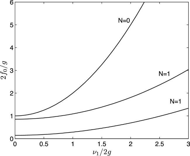
Figure 2. Parameter constraints between 2f0/g and ν1/2g for exact solutions with N1 = 0, 1.
Under these constraints λ1 = f0/g, the solution is
$\begin{eqnarray}\begin{array}{rcl}{a}_{1,1}(t) & = & \displaystyle \frac{{{\rm{e}}}^{-{\rm{i}}\tfrac{{f}_{0}}{2}t}}{{(1-{\rm{i}}gt)}^{(2{N}_{1}+3)/4}{(1+{\rm{i}}gt)}^{(2{N}_{1}+1)/4}}\\ & & \times \displaystyle \sum _{n=0}^{{N}_{1}}\displaystyle \frac{{h}_{n}}{{2}^{n}}{(1-{\rm{i}}gt)}^{n}.\end{array}\end{eqnarray}$
Choosing λ1 = -f0/g, condition (13) gives f1 = -(2N2 + 1)g. For N2 = N1 + 1, identical constraints arise, yielding a second solution
$\begin{eqnarray}\begin{array}{rcl}{a}_{1,2}(t) & = & \displaystyle \frac{{{\rm{e}}}^{{\rm{i}}\tfrac{{f}_{0}}{2}t}}{{(1-{\rm{i}}gt)}^{(2{N}_{1}+3)/4}{(1+{\rm{i}}gt)}^{(2{N}_{1}+1)/4}}\\ & & \times \displaystyle \sum _{n=0}^{{N}_{1}+1}\displaystyle \frac{{h}_{n}}{{2}^{n}}{(1-{\rm{i}}gt)}^{n}.\end{array}\end{eqnarray}$
The general solution combines these
$\begin{eqnarray}{a}_{1}(t)={c}_{1}{a}_{1,1}(t)+{c}_{2}{a}_{1,2}(t).\end{eqnarray}$
If we assume that the initial states are a1(t0) = 1 and a2(t0) = 0, we then obtain
$\begin{eqnarray}{c}_{1}=-\frac{{\dot{a}}_{1,2}({t}_{0})+f({t}_{0}){a}_{1,2}({t}_{0})/2}{\dot{{a}_{1,2}}({t}_{0}){a}_{1,2}({t}_{0})-{a}_{1,2}({t}_{0}){a}_{1,1}({t}_{0})},\end{eqnarray}$
$\begin{eqnarray}{c}_{2}=\frac{{\dot{a}}_{1,1}({t}_{0})+f({t}_{0}){a}_{1,2}({t}_{0})/2}{{\dot{a}}_{1,1}({t}_{0}){a}_{1,2}({t}_{0})-{a}_{1,2}({t}_{0}){a}_{1,1}({t}_{0})}.\end{eqnarray}$
The asymptotic behavior (t) yields |a1,1| → 0 and $| {a}_{1,2}| \to | {h}_{{N}_{1}+1}/{2}^{{N}_{1}+1}| $, giving the final probability
$\begin{eqnarray}{P}_{1}^{f}={\left|\frac{{c}_{2}{h}_{{N}_{1}+1}}{{2}^{{N}_{1}+1}}\right|}^{2}.\end{eqnarray}$
These results provide an analytical study on the parameter dependence of the probabilities |a1,2|2 and ${P}_{1,2}^{f}$.
To illustrate this, we discuss the simple case of N1 = 0 as an example. In this case, we have f1 = -3g and ${f}_{0}=({\nu }_{1}^{2}+4{g}^{2})/8g$. The solutions are given by
$\begin{eqnarray}{a}_{1,1}(t)=\displaystyle \frac{{{\rm{e}}}^{-{\rm{i}}\tfrac{{\nu }_{1}^{2}+4{g}^{2}}{16g}t}}{{(1-{\rm{i}}gt)}^{3/4}{(1+{\rm{i}}gt)}^{1/4}},\end{eqnarray}$
$\begin{eqnarray}\begin{array}{rcl}{a}_{1,2}(t) & = & \displaystyle \frac{{{\rm{e}}}^{{\rm{i}}\tfrac{{\nu }_{1}^{2}+4{g}^{2}}{16g}t}}{{(1-{\rm{i}}gt)}^{3/4}{(1+{\rm{i}}gt)}^{1/4}}\\ & & \times \left(1-\displaystyle \frac{4{g}^{2}+{\nu }_{1}^{2}}{8{g}^{2}}(1-{\rm{i}}gt)\right),\end{array}\end{eqnarray}$
with Wronskian
$\begin{eqnarray}\begin{array}{rcl}W & = & {a}_{1,1}(t)\displaystyle \frac{{\rm{d}}}{{\rm{d}}t}{a}_{1,2}(t)-{a}_{1,2}(t)\displaystyle \frac{{\rm{d}}}{{\rm{d}}t}{a}_{1,1}(t)\\ & & =\displaystyle \frac{{\rm{i}}}{64{g}^{3}}\displaystyle \frac{({\nu }_{1}^{2}+4{g}^{2})}{\sqrt{1+{g}^{2}{t}^{2}}}.\end{array}\end{eqnarray}$
This nonzero Wronskian means that a1,1(t) and a1,2(t) are linearly independent. Complete exact analytical solutions to a1(t) are thus obtained. The initial conditions of a1(t0) = 1 and a2(t0) = 0 yield the final transition probability
$\begin{eqnarray}{P}_{1}^{f}=1-\frac{16{\nu }_{1}^{2}{g}^{2}}{(1+{g}^{2}{t}_{0}^{2}){(4{g}^{2}+{\nu }_{1}^{2})}^{2}}.\end{eqnarray}$
When t0 → -, ${P}_{1}^{f}=1$ for arbitrary ν1 and g, indicating complete population revival (CPR). This arises because f(t) changes sign twice (at ${t}_{b}=\pm \sqrt{-({f}_{0}+{f}_{1})/({f}_{0}g)}$ for f0 > 0, f0 + f1 < 0 or f0 > 0, f0 + f1 > 0), leading to two avoided crossings in the adiabatic energies
$\begin{eqnarray}{E}_{\pm }^{\mathrm{ad}}(t)=\pm \displaystyle \frac{1}{2}\sqrt{{f}^{2}(t)+{\nu }^{2}(t)}.\end{eqnarray}$
Adiabatic following through dual crossings enables CPR. Figures 3(a) and (c) shows bare energies E± = ±f(t)/2 and adiabatic energies ${E}_{\pm }^{\mathrm{ad}}(t)$, and figure 3(b) displays an imperfect CPR for t0 = -100, with ${f}_{0}/g=({\nu }_{1}^{2}+4{g}^{2})/(8{g}^{2})$, f1/g = -3, ν1/g = 4/5, and g = 1. Figures 3(c) and (d) show complete population inversion (CPI) for t0 = 0, and ν1/g = 2.
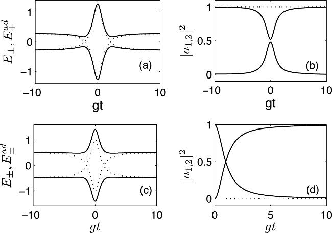
Figure 3. (a) and (c) Bare (E±, dotted) and adiabatic (${E}_{\pm }^{\mathrm{ad}}$, solid) energies. (b) and (d) Time evolution of the probability P1(t) = |a1(t)|2. In the dual-crossing case (a), (b), an imperfect CPR appears for gt0 = -100. In the single-crossing case (c), (d), CPI appears for t0 = 0. Parameters: ${f}_{0}/g=({\nu }_{1}^{2}+4{g}^{2})/8{g}^{2}$, f1/g = -3, g = 1, ν1/g = 4/5 (a), (b) and ν1/g = 2 (c), (d). In (b) and (d), the dotted lines are for the final population.
Additionally, a key question is whether exact results can be obtained when parameters deviate from termination conditions. Under general parameter conditions, the analytical solutions for a1,2 are expressed in terms of the CHFs, as given in equation (12). Here, we provide an example where an explicit exact solution for the probability |a1|2 is derived under such deviations. Here we present an example where an exact solution to the probability |a1|2 can be obtained in an explicit form when the relevant parameters deviate from termination conditions. For f0/g = 1, f1/g = -2, ν1/g = 1, the probability |a1|2 is
$\begin{eqnarray}{P}_{1}(t)=\frac{1}{2}\left(1-\frac{gt}{\sqrt{1+{g}^{2}{t}^{2}}}\right).\end{eqnarray}$
As t, ${P}_{1}^{f}\to 0$, indicating CPI. Furthermore, dual avoided crossings arise for this set of parameters. Figure 4 demonstrates CPI for f0/g = 1, f1/g = -2, and ν1/g = 1, despite the occurrence of two avoided crossings. This implies that two avoided crossings do not universally guarantee CPR.
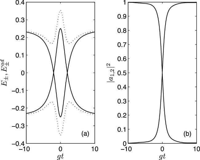
Figure 4. (a) Bare (dotted) and adiabatic (solid) energies. (b) Probability P1(t) = |a(t)|2 for gt0 = -100. Parameters: f0/g = 1, f1/g = -2, ν1/g = 1, and g = 1.

3. Conclusion

This study investigates a mixed Lorentzian TLM describing the dynamics of a two-level quantum system driven by a nonresonant laser pulse exhibiting Lorentzian frequency modulation and sub-Lorentzian amplitude modulation. A complete set of analytical solution for the system dynamics, explicitly expressed in terms of CHFs, is derived. This result identifies a novel class of ESTD TLMs in principle. Given the rapid advancement in laser technology, this mixed Lorentzian model could hold significant potential for experimental realization.
Although the asymptotic properties of CHFs are less comprehensively characterized than those of classical hypergeometric functions, they reduce to finite series under specific termination conditions. This reduction imposes an infinite set of parameter constraints, enabling exact analytical solutions. Under these constrained parameters, the instantaneous adiabatic energy levels exhibit two avoided crossings during the temporal evolution of the pulse. This characteristic double avoided crossing significantly influences the final transition probabilities between the two quantum levels; their detailed parametric dependence was analyzed using a concrete example. Furthermore, when parameters deviate from the termination constraints, an exact analytical expression for the transition probabilities in a simple form is presented.
Our method is directly applicable to the double Lorentzian TLM (see Appendix B). Moreover, it also solves the case of a TLM with only Lorentzian-modulated frequency (see Appendix C). We note that the standard Lorentzian TLM, characterized by constant detuning and Lorentzian amplitude modulation, can be mapped via a suitable transformation to a TLM with Lorentzian-modulated frequency and constant amplitude. Consequently, such a single Lorentzian frequency-modulated TLM includes the standard Lorentzian TLM as a special case.
The predictions presented in this work are promising candidates for experimental verification in established platforms such as quantum dots [48, 49], superconducting qubits [50], Nitrogen-Vacuum (NV) centers [51], and ultracold atoms [52]. Verification in these systems would significantly enhance the understanding of quantum control in two-level systems.

Appendix A Derivation of the parameters λ1,2,3

Here we present a method to determine the parameters λ1,2,3. The derivation begins with appropriate transformations of t and a1(t)

$\begin{eqnarray}z=\displaystyle \frac{1}{2}(1-{\rm{i}}gt),{a}_{1}(z)={{\rm{e}}}^{{\lambda }_{1}z}{z}^{{\lambda }_{2}}{(1-z)}^{{\lambda }_{3}}\phi (z),\end{eqnarray}$
where Φ(z) must satisfy the CHE
$\begin{eqnarray}\frac{{{\rm{d}}}^{2}\phi }{{\rm{d}}{z}^{2}}+\left(\alpha +\frac{\beta +1}{z}+\frac{\gamma +1}{z-1}\right)\frac{{\rm{d}}\phi }{{\rm{d}}z}+\frac{pz+q}{z(z-1)}\phi =0,\end{eqnarray}$
where p = δ + α(β + $\gamma$ + 2)/2 and q = η + β/2 + ($\gamma$ - α)(β + 1)/2. Substituting the transformations into equation (4) yields
$\begin{eqnarray}\frac{{{\rm{d}}}^{2}}{{\rm{d}}{z}^{2}}\phi (z)+P(z)\frac{{\rm{d}}}{{\rm{d}}z}\phi (z)+Q(z)\phi (z)=0,\end{eqnarray}$
where
$\begin{eqnarray}P(z)=2{\lambda }_{1}+\frac{1/2+2{\lambda }_{2}}{z}+\frac{1/2+2{\lambda }_{3}}{z-1},\end{eqnarray}$
$\begin{eqnarray}Q(z)=\frac{{d}_{4}{z}^{4}+{d}_{3}{z}^{3}+{d}_{2}{z}^{2}+{d}_{1}z+{d}_{0}}{16{g}^{2}{z}^{2}{(z-1)}^{2}},\end{eqnarray}$
and the coefficients dk are given by
$\begin{eqnarray}{d}_{4}=-16({f}_{0}-g{\lambda }_{1})({f}_{0}+g{\lambda }_{1}),\end{eqnarray}$
$\begin{eqnarray}{d}_{3}=16(2{f}_{0}^{2}-{f}_{0}g+{g}^{2}{\lambda }_{1}(1-2{\lambda }_{1}+2{\lambda }_{2}+2{\lambda }_{3})),\end{eqnarray}$
$\begin{eqnarray}\begin{array}{rcl}{d}_{2} & = & -4(4{f}_{0}^{2}-2{f}_{0}({f}_{1}+3g)-{\nu }_{1}^{2}-2{g}^{2}(2{\lambda }_{1}^{2}\\ & & +2{({\lambda }_{2}+{\lambda }_{3})}^{2}-{\lambda }_{1}(3+8{\lambda }_{2}+4{\lambda }_{3}))),\end{array}\end{eqnarray}$
$\begin{eqnarray}\begin{array}{rcl}{d}_{1} & = & -4(2{f}_{0}({f}_{1}+g)+{\nu }_{1}^{2}+g({f}_{1}-2g({\lambda }_{1}\\ & & +{\lambda }_{2}+4{\lambda }_{1}{\lambda }_{2}-4{\lambda }_{2}({\lambda }_{2}+{\lambda }_{3})))),\end{array}\end{eqnarray}$
$\begin{eqnarray}{d}_{0}=-({f}_{1}-4g{\lambda }_{2})({f}_{1}-2g+4g{\lambda }_{2}).\end{eqnarray}$
Comparing P(z) with the coefficients in α + (1 + β)/z + (1 + $\gamma$)/(z - 1) gives the CHE parameters
$\begin{eqnarray}\alpha =2{\lambda }_{1},\beta =-1/2+2{\lambda }_{2},\gamma =-1/2+2{\lambda }_{3}.\end{eqnarray}$
To satisfy Q(z) = (pz + q)/z(z - 1), we require
$\begin{eqnarray}\displaystyle \sum _{k=0}^{4}{d}_{k}{z}^{k}=16{g}^{2}z(z-1)(pz+q).\end{eqnarray}$
Equating coefficients results in five conditions
$\begin{eqnarray}({f}_{0}-g{\lambda }_{1})({f}_{0}+g{\lambda }_{1})=0,\end{eqnarray}$
$\begin{eqnarray}({f}_{1}-4g{\lambda }_{2})({f}_{1}-2g+4g{\lambda }_{2})=0,\end{eqnarray}$
$\begin{eqnarray}\begin{array}{l}16{g}^{2}p-{d}_{3}=0,16{g}^{2}q-{d}_{1}=0,\\ 16{g}^{2}(q-p)-{d}_{2}=0.\end{array}\end{eqnarray}$
From equation (A13), we have
$\begin{eqnarray}{\lambda }_{1}=\pm \frac{{f}_{0}}{g}.\end{eqnarray}$
From equation (A14), we get
$\begin{eqnarray}{\lambda }_{2}=\frac{{f}_{1}}{4g},-\frac{{f}_{1}-2g}{4g}.\end{eqnarray}$
Equation (A15) implies p = d3/16g2, q = d1/16g2, and ${d}_{1}-{d}_{3}-{d}_{2}={f}_{1}({f}_{1}+2g)+8{g}^{2}({\lambda }_{3}-2{\lambda }_{3}^{2})=0$. Accordingly, the parameter λ3 is given by
$\begin{eqnarray}{\lambda }_{3}=-\frac{{f}_{1}}{4g},\frac{{f}_{1}+2g}{4g}.\end{eqnarray}$
Once the three parameters λ1,2,3 are given, the relevant parameters δ and η are given by
$\begin{eqnarray}\delta =-\frac{{f}_{0}}{g},\end{eqnarray}$
$\begin{eqnarray}\eta =\frac{4{f}_{0}({f}_{1}+g)+{f}_{1}^{2}+2{\nu }_{1}^{2}+3{g}^{2}}{8{g}^{2}}.\end{eqnarray}$

In principle, we have eight sets of the possible combinations of λ1,2,3. To construct a complete set of analytical solutions, we select

$\begin{eqnarray}{\lambda }_{1}=\pm \frac{{f}_{0}}{g},{\lambda }_{2}=\frac{{f}_{1}}{4g},{\lambda }_{3}=\frac{{f}_{1}+2g}{4g}.\end{eqnarray}$
It is note that one may make the alternative choice
$\begin{eqnarray}{\lambda }_{1}=\pm \frac{{f}_{0}}{g},{\lambda }_{2}=-\frac{{f}_{1}-2g}{4g},{\lambda }_{3}=-\frac{{f}_{1}}{4g},\end{eqnarray}$
yielding identical results under the replacements of f0,1 → -f0,1. However, such a choice of the parameters will lead to the similar results. For example, when N = 0, we have f1 = 3g and ${f}_{0}=({\nu }_{1}^{2}+4{g}^{2})/8g$.

Appendix B Double Lorentzian TLMll

Here we will show that our approach is applicable to the double Lorentzian TLM, as given in equation (6). We make use of the same transformations in equation (A1), and then obtain the same equation structure as equation (A3) but with

$\begin{eqnarray}P(z)=2{\lambda }_{1}+\frac{1+2{\lambda }_{2}}{z}+\frac{1+2{\lambda }_{3}}{z-1},\end{eqnarray}$
which yields the relevant parameters in the CHE
$\begin{eqnarray}\alpha =2{\lambda }_{1},\beta =2{\lambda }_{2},\gamma =2{\lambda }_{3}.\end{eqnarray}$
In equation (A3), the coefficients dk in Q(z) are given by
$\begin{eqnarray}{d}_{4}=-16({f}_{0}-g{\lambda }_{1})({f}_{0}+g{\lambda }_{1}),\end{eqnarray}$
$\begin{eqnarray}{d}_{3}=32(2{f}_{0}^{2}-{f}_{0}g+{g}^{2}{\lambda }_{1}(1-{\lambda }_{1}+2{\lambda }_{2}+2{\lambda }_{3})),\end{eqnarray}$
$\begin{eqnarray}\begin{array}{rcl}{d}_{2} & = & -8(2{f}_{0}^{2}-{f}_{0}({f}_{1}+6g)-2{g}^{2}({\lambda }_{1}^{2}+{({\lambda }_{2}+{\lambda }_{3})}^{2}\\ & & +{\lambda }_{2}+{\lambda }_{3}-{\lambda }_{1}(3+4{\lambda }_{2}+2{\lambda }_{3}))),\end{array}\end{eqnarray}$
$\begin{eqnarray}{d}_{1}=-8({f}_{0}({f}_{1}+2g)+2{g}^{2}(1+2{\lambda }_{2})({\lambda }_{2}+{\lambda }_{3}-{\lambda }_{1})),\end{eqnarray}$
$\begin{eqnarray}{d}_{0}=-({f}_{1}^{2}+{\nu }_{1}^{2}-16{g}^{2}{\lambda }_{2}^{2}).\end{eqnarray}$
Now the conditions for determining the parameters λ1,2,3 become
$\begin{eqnarray}({f}_{0}-g{\lambda }_{1})({f}_{0}+g{\lambda }_{1})=0,\end{eqnarray}$
$\begin{eqnarray}({f}_{1}^{2}+{\nu }_{1}^{2}-16{g}^{2}{\lambda }_{2}^{2})=0,\end{eqnarray}$
$\begin{eqnarray}\begin{array}{l}16{g}^{2}p-{d}_{3}=0,16{g}^{2}q-{d}_{1}=0,\\ 16{g}^{2}(q-p)-{d}_{2}=0.\end{array}\end{eqnarray}$
From conditions equations (B8) and (B9), we obtain at once
$\begin{eqnarray}{\lambda }_{1}=\pm \frac{{f}_{0}}{g},{\lambda }_{2}=\pm \frac{\sqrt{{f}_{1}^{2}+{\nu }_{1}^{2}}}{4g}.\end{eqnarray}$
From condition equation (B10), we get p = d3/16g2, q = d1/16g2, and thus the relation ${d}_{1}-{d}_{3}-{d}_{2}\,={f}_{1}^{2}+{\nu }_{1}^{2}-16{g}^{2}{\lambda }_{3}^{2}=0$. This gives
$\begin{eqnarray}{\lambda }_{3}=\pm \frac{\sqrt{{f}_{1}^{2}+{\nu }_{1}^{2}}}{4g}.\end{eqnarray}$
Once the three parameters λ1,2,3 are specified, the parameters δ and η are given by
$\begin{eqnarray}\delta =-\frac{2{f}_{0}}{g},\end{eqnarray}$
$\begin{eqnarray}\eta =\frac{{f}_{0}{f}_{1}+2{f}_{0}g+4{g}^{2}{\lambda }_{2}^{2}}{2{g}^{2}}.\end{eqnarray}$
To derive a complete set of analytical solutions, we may select [45-47]
$\begin{eqnarray}{\lambda }_{1}=\pm \frac{{f}_{0}}{g},{\lambda }_{2}={\lambda }_{3}=-\frac{\sqrt{{f}_{1}^{2}+{\nu }_{1}^{2}}}{4g}.\end{eqnarray}$
For the case of λ1 = -f0/g, applying condition equation (13) produces
$\begin{eqnarray}\sqrt{{f}_{1}^{2}+{\nu }_{1}^{2}}=2({N}_{1}+2)g.\end{eqnarray}$
Similarly, in the case of λ1 = f0/g, we have
$\begin{eqnarray}\sqrt{{f}_{1}^{2}+{\nu }_{1}^{2}}=2{N}_{2}g.\end{eqnarray}$
Condition (equation (14)) provides the parameter constraints for the exact analytical solutions. In the case of N2 = N1 + 2, we obtain two linearly independent solutions to a1(t). In the simplest nontrivial three cases of N = 0, 1, 2, we have the same parameter constraints in prior work in [31].

Appendix C Single Lorentzian TLM with Lorentzian frequency modulation

In this section, we demonstrate that our approach is applicable to another class of time-dependent TLM with constant amplitude, where f(t) and ν(t) adopt the form

$\begin{eqnarray}f(t)={f}_{0}+\frac{{f}_{1}}{1+{g}^{2}{t}^{2}},\nu (t)={\nu }_{0}.\end{eqnarray}$
We call it single Lorentzian TLM. By swapping the Pauli operators σx and σz in equation (1), the resulting "single Lorentzian TLM" Hamiltonian specifically models a two-level system driven by a laser pulse that has a constant detuning and a Lorentzian amplitude modulation. The standard Lorentzian TLM refers to the limiting case of this model where the detuning parameter f0 is exactly zero.

For this case, we apply the transformations in equation (A1) and obtain the same equation structure as equation (A3) but with

$\begin{eqnarray}P(z)=2{\lambda }_{1}+\frac{2{\lambda }_{2}}{z}+\frac{2{\lambda }_{3}}{z-1},\end{eqnarray}$
which yields the relevant parameters in the CHE
$\begin{eqnarray}\alpha =2{\lambda }_{1},\beta =-1+2{\lambda }_{2},\gamma =-1+2{\lambda }_{3}.\end{eqnarray}$
Now in equation (A3), the coefficients dk in Q(z) are given by
$\begin{eqnarray}{d}_{4}=-16({f}_{0}^{2}+{\nu }_{0}^{2}-{g}^{2}{\lambda }_{1}^{2}),\end{eqnarray}$
$\begin{eqnarray}{d}_{3}=32({f}_{0}^{2}+{\nu }_{0}^{2}+{g}^{2}{\lambda }_{1}({\lambda }_{2}+{\lambda }_{3}-{\lambda }_{1})),\end{eqnarray}$
$\begin{eqnarray}\begin{array}{rcl}{d}_{2} & = & -8(2{f}_{0}^{2}-{f}_{0}{f}_{1}-{\nu }_{0}^{2}-2({\nu }_{0}^{2}-{g}^{2}({\lambda }_{1}^{2}+({\lambda }_{2}\\ & & +{\lambda }_{3}-1)({\lambda }_{2}+{\lambda }_{3})-2{\lambda }_{1}(2{\lambda }_{2}+{\lambda }_{3}))),\end{array}\end{eqnarray}$
$\begin{eqnarray}{d}_{1}=-8({f}_{0}{f}_{1}+g({f}_{1}+4g{\lambda }_{2}({\lambda }_{2}+{\lambda }_{3}-{\lambda }_{1}-1))),\end{eqnarray}$
$\begin{eqnarray}{d}_{0}=-({f}_{1}-4g{\lambda }_{2})({f}_{1}-4g+4g{\lambda }_{2}).\end{eqnarray}$
The conditions for the parameters λ1,2,3 are
$\begin{eqnarray}({f}_{0}^{2}+{\nu }_{0}^{2}-{g}^{2}{\lambda }_{1}^{2})=0,\end{eqnarray}$
$\begin{eqnarray}({f}_{1}-4g{\lambda }_{2})({f}_{1}-4g+4g{\lambda }_{2})=0,\end{eqnarray}$
$\begin{eqnarray}\begin{array}{l}16{g}^{2}p-{d}_{3}=0,16{g}^{2}q-{d}_{1}=0,\\ 16{g}^{2}(q-p)-{d}_{2}=0.\end{array}\end{eqnarray}$
From condition (C9), we obtain
$\begin{eqnarray}{\lambda }_{1}=\pm \frac{\sqrt{{f}_{0}^{2}+{\nu }_{0}^{2}}}{g}.\end{eqnarray}$
Condition (equation (C10)) yields
$\begin{eqnarray}{\lambda }_{2}=\frac{{f}_{1}}{4g},-\frac{{f}_{1}-4g}{4g}.\end{eqnarray}$
Now from condition (equation (C11)), we have p = d3/16g2, q = d1/16g2, and thus the relation ${d}_{1}-{d}_{3}-{d}_{2}={f}_{1}({f}_{1}+4g)+16{g}^{2}({\lambda }_{3}-2{\lambda }_{3}^{2})=0$, thereby leading to
$\begin{eqnarray}{\lambda }_{3}=-\frac{{f}_{1}}{4g},\frac{{f}_{1}+4g}{4g}.\end{eqnarray}$
Finally, the parameters δ and η are given by
$\begin{eqnarray}\delta =0,\end{eqnarray}$
$\begin{eqnarray}\eta =\frac{4{f}_{0}{f}_{1}+{f}_{1}^{2}+4{g}^{2}}{8{g}^{2}}.\end{eqnarray}$
To derive a complete set of analytical solutions, we may select [45-47]
$\begin{eqnarray}{\lambda }_{1}=\pm \frac{\sqrt{{f}_{0}^{2}+{\nu }_{0}^{2}}}{g},{\lambda }_{2}=\frac{{f}_{1}}{4g},{\lambda }_{3}=\frac{{f}_{1}+4g}{4g}.\end{eqnarray}$
Applying condition (equation (13)) yields
$\begin{eqnarray}{f}_{1}=-2(N+1)g.\end{eqnarray}$
Condition (14) provides an additional parameter constraint. In the simplest nontrivial three cases of N = 1, 2, 3, we have
$\begin{eqnarray}\frac{{f}_{0}}{g}-1=0,\end{eqnarray}$
$\begin{eqnarray}{\left(\frac{{f}_{0}}{g}-\frac{3}{2}\right)}^{2}-\frac{1}{8}\left(\frac{{\nu }_{0}^{2}}{{g}^{2}}+6\right)=0,\end{eqnarray}$
$\begin{eqnarray}\left(\frac{{f}_{0}}{g}-2\right)\frac{{\nu }_{0}^{2}}{{g}^{2}}-3\left(\frac{{f}_{0}^{3}}{{g}^{3}}-6\frac{{f}_{0}^{2}}{{g}^{2}}+9\frac{{f}_{0}}{g}-3\right)=0.\end{eqnarray}$
In the simple case of N = 1, we have f1 = -4g and f0 = g. The complete analytical solutions for a1(t) are given by
$\begin{eqnarray}{a}_{1,1}(t)=\displaystyle \frac{{{\rm{e}}}^{-{\rm{i}}\sqrt{{g}^{2}+{\nu }_{0}^{2}}t/2}}{1-{\rm{i}}gt}(1-\displaystyle \frac{\sqrt{{g}^{2}+{\nu }_{0}^{2}}}{2g}(1-{\rm{i}}gt)),\end{eqnarray}$
$\begin{eqnarray}{a}_{1,2}(t)=\displaystyle \frac{{{\rm{e}}}^{{\rm{i}}\sqrt{{g}^{2}+{\nu }_{0}^{2}}t/2}}{1-{\rm{i}}gt}(1+\displaystyle \frac{\sqrt{{g}^{2}+{\nu }_{0}^{2}}}{2g}(1-{\rm{i}}gt)).\end{eqnarray}$

This work was supported by the National Natural Science Foundation of China under Grant No. 11965011.

[1]
Shapiro M, Brumer P 2003 Principles of the Quantum Control of Molecular Processes Wiley Press

[2]
Chua S-I, Telnov D A 2004 Beyond the Floquet theorem: generalized Floquet formalisms and quasienergy methods for atomic and molecular multiphoton processes in intense laser fields Phys. Rep. 390 1

DOI

[3]
Grifoni M, Hänggi P 1998 Driven quantum tunneling Phys. Rep. 304 229

DOI

[4]
Landau L D 1932 On the theory of transfer of energy at collisions II Phys. Z. Sowjetunion 2 46

[5]
Zener C 1932 Non-adiabatic crossing of energy levels Proc. R. Soc. London, Ser. A 137 696

DOI

[6]
Rosen N, Zener C 1932 Double Stern-Gerlach experiment and related collision phenomena Phys. Rev. 40 502

DOI

[7]
Nikitin E E 1962 The probability of nonadiabatic transitions in the case of nondivergent terms Opt. Spectrosc. 13 431

[8]
Demkov Y N 1964 Detachment of electrons in slow collisions between negative ions and atoms Sov. Phys. JETP 18 138

[9]
Demkov Y N, Kunike M 1969 Hypergeometric models for the two-state approximation in collision theory Vestn Leningr. Univ. Fis. Khim. 16 39

[10]
Bambini A, Berman P R 1981 Analytic solutions to the two-state problem for a class of coupling potentials Phys. Rev. A 23 2496

DOI

[11]
Bambini A, Lindberg M 1984 Transition probability of a two-level atom interacting with a time-symmetric pulse Phys. Rev. A 30 794

DOI

[12]
Hioe F T 1984 Solution of Bloch equations involving amplitude and frequency modulations Phys. Rev. A 30 2100

DOI

[13]
Robinson E J 1985 Two-level systems driven by modulated pulses Phys. Rev. A 31 3986

DOI

[14]
Hioe F T, Carroll C E 1985 Two-state problems involving arbitrary amplitude and frequency modulations Phys. Rev. A 32 1541

DOI

[15]
Carroll C E, Hioe F T 1986 A new class of analytic solutions of the two-state problem J. Phys. A: Math. Gen. 19 3579

DOI

[16]
Carroll C E, Hioe F T 1990 Analytic solution of the two-state problem Phys. Rev. A 41 2835

DOI

[17]
Allen L, Eberly J H 1987 Optical Resonance and Two-level Atoms Dover Press

[18]
Ishkhanyan A M 1997 The integrability of the two-state problem in terms of confluent hypergeometric functions J. Phys. A: Math. Gen. 30 1203

DOI

[19]
Ishkhanyan A M 2000 New classes of analytic solutions of the two-level problem J. Phys. A: Math. Gen. 33 5539

DOI

[20]
Vitanov N V 2007 Complete population inversion by a phase jump: an exactly soluble model New J. Phys. 9 58

DOI

[21]
Torosov B T, Vitanov N V 2007 Coherent control of a quantum transition by a phase jump Phys. Rev. A 76 053404

DOI

[22]
Ishkhanyan A M, Suominen K-A 2001 Solutions of the two-level problem in terms of biconfluent Heun functions J. Phys. A: Math. Gen. 34 6301

DOI

[23]
Jha P K, Rostovtsev Y V 2010 Coherent excitation of a two-level atom driven by a far-off-resonant classical field: analytical solutions Phys. Rev. A 81 033827

DOI

[24]
Jha P K, Rostovtsev Y V 2010 Analytical solutions for a two-level system driven by a class of chirped pulses Phys. Rev. A 82 015801

DOI

[25]
Xie Q, Hai W 2010 Analytical results for a monochromatically driven two-level system Phys. Rev. A 82 032117

DOI

[26]
Ishkhanyan A M, Grigoryan A E 2014 Fifteen classes of solutions of the quantum two-state problem in terms of the confluent Heun function J. Phys. A: Math. Theor. 47 465205

DOI

[27]
Shahverdyan T A, Ishkhanyan T A, Grigoryan A E, Ishkhanyan A M 2015 Analytic solutions of the quantum two-state problem in terms of the double-, bi- and tri-confluent Heun functions J. Contemp. Phys. 50 211

DOI

[28]
Ishkhanyan A M, Shahverdyan T A, Ishkhanyan A M 2015 Thirty five classes of solutions of the quantum time-dependent two-state problem in terms of the general Heun functions Eur. Phys. J. D 69 10

DOI

[29]
Xie Q 2018 Analytical results for periodically-driven two-level models in relation to Heun functions Pramana-J. Phys. 91 19

DOI

[30]
Deng H, Shen Z, Xie Q 2019 Exact Floquet solutions in a periodically driven non-Hermitian parity-time symmetric two-level model Phys. Scr. 94 125003

DOI

[31]
Xie Q, Liu X 2020 Exact analytical results for a two-level quantum system under a Lorentzian-shaped pulse field Chin. Phys. B 29 060305

DOI

[32]
Garanin D A, Schilling R 2002 Inverse problem for the Landau-Zener effect Europhys. Lett. 59 7

DOI

[33]
Yang X, Wu Y 2006 Efficient approach to seek exact analytical solutions of periodically driven two-level systems J. Phys. B: At. Mol. Opt. Phys. 39 2285

DOI

[34]
Gangopadhyay A, Dzero M, Galitski V 2010 Exact solution for quantum dynamics of a periodically driven two-level system Phys. Rev. B 82 024303

DOI

[35]
Barnes E, Sarma S D 2012 Analytically solvable driven time-dependent two-level quantum systems Phys. Rev. Lett. 109 060401

DOI

[36]
Barnes E 2013 Analytically solvable two-level quantum systems and Landau-Zener interferometry Phys. Rev. A 88 013818

DOI

[37]
Conover C W S 2011 Effects of pulse shape on strongly driven two-level systems Phys. Rev. A 84 063416

DOI

[38]
Bason M G, Viteau M, Malossi N, Huillery P, Arimondo E, Ciampini D, Fazio R, Giovannetti V, Mannella R, Morsch Q 2012 High-fidelity quantum driving Nat. Phys. 8 147

DOI

[39]
Chen Y-Y, Feng X-L, Liu C 2016 Generation of nonlinear vortex precursors Phys. Rev. Lett. 117 023901

DOI

[40]
Zhang C, Liu C 2019 Origin of unusual even-order harmonic generation by a vortex laser Opt. Express 27 37034

DOI

[41]
Liu C, Gong S, Li R, Xu Z 2004 Coherent control in the generation of harmonics and hyper-Raman lines from a strongly driven two-level atom Phys. Rev. A 69 023406

DOI

[42]
Wang H, Li N, Bai Y, Liu P, Wang S, Liu C 2017 Generation of largely elliptically polarized terahertz radiation from laser-induced plasma Opt. Express 25 30987

DOI

[43]
Wang H, Bai Y, Wu E, Wang Z, Liu P, Liu C 2018 Terahertz necklace beams generated from two-color vortex-laser-induced air plasma Phys. Rev. A 98 013857

DOI

[44]
Zhang X, Du H, Wang H, Guo H, Liu C 2023 Residual current under the combined effect of carrier envelope phase and chirp: phase shift and peak enhancement Opt. Express 31 26879

DOI

[45]
Ronveaux A 1995 Heun's Differential Equations Oxford University Press

[46]
Slavyanov S Y, Lay W 2000 Special Functions: A Unified Theory Based on Singularities Oxford University Press

[47]
Olver J W F, Lozier W D, Boisvert F R, Clark W C 2010 NIST Handbook of Mathematical Functions Cambridge University Press

[48]
Gong M, Zhang W, Guo G-C, He L 2011 Exciton polarization, fine-structure splitting, and the asymmetry of quantum dots under uniaxial stress Phys. Rev. Lett. 106 227401

DOI

[49]
Gong M, Hofer B, Zallo E, Trotta R, Luo J-W, Schmidt O G, Zhang C 2014 Statistical properties of exciton fine structure splitting and polarization angles in quantum dot ensembles Phys. Rev. B 89 205312

DOI

[50]
Wu Z, Hu C, Wang T, Chen Y, Li Y, Zhao L, X-Y, Peng X 2024 Experimental quantum simulation of multicriticality in closed and open Rabi model Phys. Rev. Lett. 133 173602

DOI

[51]
Yoshihara F, Fuse T, Ashhab S, Kakuyanagi K, Saito S, Semba K 2017 Superconducting qubit-oscillator circuit beyond the ultrastrong-coupling regime Nat. Phys. 13 44

DOI

[52]
Koch J, Hunanyan G R, Ockenfels T, Rico E, Solano E, Weitz M 2023 Quantum Rabi dynamics of trapped atoms far in thedeep strong coupling regime Nat. Commun. 14 954

DOI

Outlines

/