


1. Introduction
One of the main modes of decay of the atomic nuclei in the region of actinides and superheavy nuclei is α-decay. Sequential α-decays to a known nucleus often serve as an experimental method to identify new isotopes of superheavy nuclei [1]. The energy released in ground-state to ground-state α-decay allows us to determine the binding energy of the parent nucleus from the known binding energy of the daughter nucleus, thereby reducing the uncertainty of theoretical models [2, 3]. Additionally, the α-decays to excited states allow us to extract the invaluable information about the structure of the daughter nucleus.
A widely used assumption in solving the problem of α-decay is that the α-particle is formed with some probability on the surface of the parent nucleus. The α-particle is confined in a potential that is well formed by attractive nuclear and repulsive Coulomb potentials. Since the potential barrier has a finite height, spontaneous decay of the system is possible. Therefore, the probability of α-decay is determined by the product of two factors: the spectroscopic factor, which gives the probability of formation of an α-particle on the surface of the nucleus and the penetrability of the potential barrier. This approach, based on the pioneering work of Gamow [4], turned out to be very successful in describing the main characteristics of α-decay. For example, the Geiger-Netall law was established, which connects the half-life with the energy Qα released in α-decay [5]. This relationship effectively explains the systematic variations in α-decay probabilities for transitions between the ground states of even-even nuclei. However, for the α-decay to excited states of daughter nuclei, sharp changes in the decay rates are observed [6].
A possible explanation for this behavior is the dependence of both the tunneling probability and the spectroscopic factor on the deformation of the parent nucleus. First, it should be taken into consideration that if the daughter nucleus is deformed, then the potential barrier is not spherically symmetric. As a consequence, the angular momentum of α-particle can change during tunneling [7]. Secondly, the deformation of the daughter nucleus leads to the fact that the α-particle is formed on the surface of the nucleus in states with different angular momenta. The interplay of these two factors determines the resulting fine structure of α-decay.
The fine structure of α-decay has attracted considerable attention in both theoretical and experimental studies. In recent years, interest in this phenomenon has been renewed, motivated by the development of advanced experimental techniques and improved theoretical frameworks. This interest arises from the fact that the fine-structure of α-decay plays a decisive role in determining the decay patterns of both neutron-deficient and superheavy nuclei [8-13]. Moreover, fine-structure studies provide valuable insight into the nature of various isomeric states and their underlying nuclear structure (see, for example, [14]).
Two primary approaches are used to address the α-decay problem: the semiclassical [15-18] and microscopic approaches. Later employing the coupled-channel formalism [19, 20], cluster mean-field description [21], and improved density-dependent cluster model [22]. However, until recently, the angular momentum dependence of the spectroscopic factor has not been taken into account explicitly. It was either assumed that all angular momenta are populated with equal probabilities as in [7, 17], or treated empirically using the Boltzmann distribution (BD) [15, 18].
It has been recognized that the angular momentum dependence of spectroscopic factor arises from the couplings between the relative motion of the α-particle and various collective excitations of daughter nucleus. Accordingly, the effect of vibrational excitations of the daughter nucleus was investigated in the frame of multichannel cluster model in [23], and the effect of rotational excitations of deformed daughter nucleus was examined in [24].
In this work, we apply the dinuclear system model (DNS) [25, 26] to directly calculate the angular momentum dependence of spectroscopic factors. The model allows us to treat the coupling between the yrast excitations of daughter nucleus and motion of α-particle on its surface in a consistent way. The role of quadrupole and octupole deformation of the daughter nucleus is analyzed. The results obtained are compared with the empirical values provided by BD.
2. Model
In the actinide mass region, the wave function of a nucleus can be represented as a superposition of the mononuclear configuration $\Psi$m and the α-cluster dinuclear system (DNS) $\Psi$α [25]:
$\begin{eqnarray}{\rm{\Psi }}=\cos \gamma {{\rm{\Psi }}}_{m}+\sin \gamma {{\rm{\Psi }}}_{\alpha },\end{eqnarray}$
where the weight of the α-cluster component (spectroscopic factor) is defined as ${S}_{\alpha }={\sin }^{2}\gamma $. To obtain Sα, one can solve the Schrödinger equation in mass asymmetry coordinate (see, for example, [7, 26]). The spectroscopic factor depends on the relative distance between the centers of the daughter nucleus and the α-particle. At distances less than touching, the α-particle dissociates and Sα decreases to zero [27]. For larger distances, the spectroscopic factor rapidly approaches unity. At touching, the probability of forming an α-particle on the surface of the heavy nucleus (α-DNS) achieves several percents. As was shown in [26], the contribution of this component is crucial to describe the formation of negative parity states in actinides. In the current calculations, however, we are not interested in the spectroscopic factor itself but rather its dependence on the angular momentum. Since the mononucleus wave function does not contribute to the α-decay, this dependence originates from the structure of the α-DNS wave function $\Psi$α.In the following, we assume that only the lowest collective excited states contribute to $\Psi$α. The degrees of freedom required for the description of the collective motion in α-DNS are related to the motion in relative distance coordinate R, to the rotation of the system as a whole described by the angles ΩR = (θR, ΦR), and to the collective rotation of the daughter nucleus described by the angles Ωh = (θh, Φh). The schematic representation of α-DNS with indication of the degrees of freedom used is shown in figure 1.
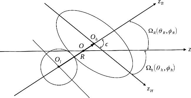
Figure 1. Schematic representation of α-DNS. The orientation of the vector R, connecting the centers of two fragment, is defined by the angles ΩR = (θR, ΦR) with respect to the laboratory system Oz. The orientation of the intrinsic coordinate system of the daughter nucleus Ohzh with respect to the laboratory system is described by the angles Ωh = (θh, Φh). The angle ε is a plane angle between R and the symmetry axis of the deformed fragment. |
The kinetic energy of the collective motion in the DNS is written as [26]: 2 ), $\mathfrak{I}$R = μR2 is the moment of inertia of rotation of the DNS as a whole. Taking into account that the light fragment of the DNS is an α-particle, the reduced mass is written as μ = m04(A - 4)/A, where m0 is the nucleon mass. In the calculations, it is preferable to use experimental values for the energies of the yrast states of the daughter nucleus. Therefore, the moment of inertia $\mathfrak{I}$h(Ih) is adjusted so that for angular momentum Ih, the last term of equation (2 ) reproduces the experimental energies E(Ih) of the corresponding yrast state of daughter nucleus:
$\begin{eqnarray}\hat{T}=-\frac{{\hslash }^{2}}{2\mu {R}^{2}}\frac{\partial }{\partial R}{R}^{2}\frac{\partial }{\partial R}+\frac{{\hslash }^{2}}{2{\Im }_{R}}{\hat{I}}_{R}^{2}+\frac{{\hslash }^{2}}{2{\Im }_{h}({I}_{h})}{\hat{I}}_{h}^{2},\end{eqnarray}$
where the angular momentum operators have the form: $\begin{eqnarray}{\hat{I}}_{i}^{2}=-\frac{1}{\sin {\theta }_{i}}\frac{\partial }{\partial {\theta }_{i}}\sin {\theta }_{i}\frac{\partial }{\partial {\theta }_{i}}-\frac{1}{{\sin }^{2}{\theta }_{i}}\frac{{\partial }^{2}}{\partial {\phi }_{i}^{2}},\quad (i=R,h).\end{eqnarray}$
In equation ( $\begin{eqnarray}{\Im }_{h}({I}_{h})=\frac{{\hslash }^{2}{I}_{h}({I}_{h}+1)}{2E({I}_{h})}.\end{eqnarray}$
Note that thus defined $\mathfrak{I}$h(Ih) allows us to include both rotational and vibrational, contributions to the energies of the yrast states of the daughter nucleus.Potential energy in general form can be presented as
$\begin{eqnarray}V(R,{{\rm{\Omega }}}_{h},{{\rm{\Omega }}}_{R})=\displaystyle \sum _{\lambda }{V}_{\lambda }(R){\left[{Y}_{\lambda }({{\rm{\Omega }}}_{h})\times {Y}_{\lambda }({{\rm{\Omega }}}_{R})\right]}_{(00)},\end{eqnarray}$
where bipolar spherical functions are defined as (see [28]) $\begin{eqnarray}\begin{array}{l}{[{Y}_{{\lambda }_{h}}({{\rm{\Omega }}}_{h})\times {Y}_{{\lambda }_{R}}({{\rm{\Omega }}}_{R})]}_{(\lambda ,m)}\\ \quad =\displaystyle \sum _{{m}_{h},{m}_{R}}{C}_{{\lambda }_{h}{m}_{h},{\lambda }_{R}{m}_{R}}^{\lambda m}{Y}_{{\lambda }_{h}{m}_{h}}({{\rm{\Omega }}}_{h}){Y}_{{\lambda }_{R}{m}_{R}}({{\rm{\Omega }}}_{R}).\end{array}\end{eqnarray}$
The functions ${\left[{Y}_{\lambda }({{\rm{\Omega }}}_{h})\times {Y}_{\lambda }({{\rm{\Omega }}}_{R})\right]}_{(00)}$ are related to the Legendre polynomials: $\begin{eqnarray}{P}_{\lambda }(\cos \varepsilon )=\frac{{(-1)}^{\lambda }}{\sqrt{2\lambda +1}}{\left[{Y}_{\lambda }({{\rm{\Omega }}}_{h})\times {Y}_{\lambda }({{\rm{\Omega }}}_{R})\right]}_{(00)},\end{eqnarray}$
where ε is a plane angle between the vector R and the symmetry axis of the daughter nucleus (see figure 1). Therefore, the angular dependence of potential energy is defined only by angle ε and expressed as $\begin{eqnarray}V(R,\varepsilon )=\displaystyle \sum _{\lambda }{(-1)}^{\lambda }\frac{\sqrt{2\lambda +1}}{4\pi }{V}_{\lambda }(R){P}_{\lambda }(\cos \varepsilon ).\end{eqnarray}$
An example of potential energy calculation is presented in figure 2 for the DNS 226Ra+α, with axially-symmetric quadrupole and octupole deformation parameters β2 = 0.164 and β3=0.113, respectively. Panel (a) shows the potential energy as a function of relative distance R calculated for ε = 0. As seen, due to the interplay between Coulomb and nuclear interactions, the potential energy exhibits a minimum at the distance Rt in the vicinity of touching configuration. In figure 2(b), the potential energy is displayed at the minimum of the pocket for each value of ε. It is seen that because of nonzero octupole deformation the potential is reflection asymmetric. The potential energy has a minimum at ε = 0 with the α-particle located at the tip of the daughter nucleus and less deep minimum at ε = π, when α-particle is located at the bottom of the daughter nucleus.
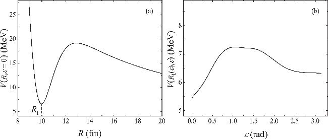
Figure 2. Potential energy V(R, ε) of DNS 226Ra+α. The dependence of potential on relative distance coordinate R for ε = 0 is shown on panel (a). The angular dependence of the potential energy in the minimum, V(Rt(ε), ε), is presented in panel (b). |
For the solution of the Schrodinger equation with Hamiltonian $\hat{H}=\hat{T}+V$, we resort to using Born-Oppenheimer approximation. In other words, we assume that motion in R is so fast that for each value of angles, the DNS achieves its equilibrium configuration which approximately corresponds to the minimum of pocket at Rt(ε). To demonstrate it, we take the potential energy of the DNS 226Ra+α presented in figure 2. From the form of the potential energy, it is clear that the wave function will be mostly localized around ε = 0 in orientation angle and around Rt(ε = 0) in the relative distance coordinate (see also discussion of figure 3). Fitting the calculated potential energy in this region by the oscillator, we obtain:
$\begin{eqnarray*}V(R,\varepsilon )\approx \frac{{C}_{R}}{2}{(R-{R}_{t}(\varepsilon =0))}^{2}+\frac{{C}_{\varepsilon }}{2}{\varepsilon }^{2},\end{eqnarray*}$
with stiffness parameters CR ≈ 14 MeV fm-2 and Cε ≈ 10 MeV rad-2. Using these values of stiffness parameters, we estimate the frequency of vibrations in relative distance coordinate R as $\hslash {\omega }_{R}=\sqrt{{C}_{R}/\mu }\approx 12$ MeV and the frequency of angular vibrations around ε = 0 as $\hslash {\omega }_{\varepsilon }\approx \sqrt{{C}_{\varepsilon }/{\Im }_{b}}\approx 1$ MeV, where ${\Im }_{b}={(1/{\Im }_{h}+1/\mu {R}_{t}^{2}(0))}^{-1}$ [26]. We see that ħωR » ħωε and motion in relative distance coordinate is indeed much faster than angular motion.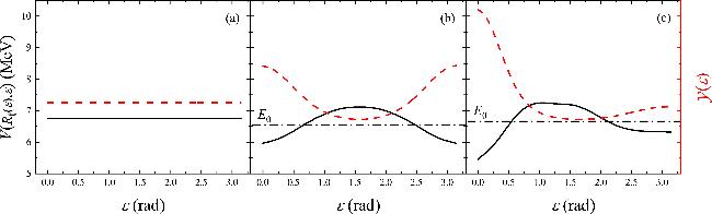
Figure 3. Potential energy V(Rt(ε), ε) (black lines) and the wave functions ${ \mathcal Y }(\varepsilon )$ (red dotted lines) are shown for 226Ra+α DNS for three different sets of 226Ra deformation parameters: panel (a): β2 = β3 = 0, panel (b): β2 = 0.164, β3 = 0, and panel (c): β2 = 0.164, β3 = 0.113. |
The wave function is then factorized as a product of wave functions in slow and fast coordinates:
$\begin{eqnarray}{{\rm{\Psi }}}_{\alpha }(R,{{\rm{\Omega }}}_{h},{{\rm{\Omega }}}_{R})=\frac{\psi (R)}{R}{ \mathcal Y }({{\rm{\Omega }}}_{h},{{\rm{\Omega }}}_{R}).\end{eqnarray}$
In the equation for the radial wave function ψ(R), the angular part of the kinetic energy is neglected, which yields the following Schrodinger equation for ψ(R): $\begin{eqnarray}\left[-\frac{{\hslash }^{2}}{2\mu }\frac{{\partial }^{2}}{\partial {R}^{2}}+V(R,\varepsilon )\right]\psi (R)=E(\varepsilon )\psi (R),\end{eqnarray}$
where E(ε) = ‹TR› + V(Rt(ε), ε). Here, the average kinetic energy ‹TR› and potential V are calculated at the minimum of the pocket for each value of ε.Assuming that ‹TR› weakly depends on ε, we write the Hamiltonian for angular vibrations in the α-DNS in the following form:
$\begin{eqnarray}\begin{array}{rcl}\hat{H} & = & \hat{T}+V({{\rm{\Omega }}}_{h},{{\rm{\Omega }}}_{R}),\\ \hat{T} & = & \frac{{\hslash }^{2}}{2\mu {R}_{t}^{2}(0)}{\hat{I}}_{R}^{2}+\frac{{\hslash }^{2}}{2{\Im }_{h}({I}_{h})}{\hat{I}}_{h}^{2},\\ V({{\rm{\Omega }}}_{h},{{\rm{\Omega }}}_{R}) & = & V({R}_{t}(\varepsilon ),\varepsilon )\\ & = & \displaystyle \sum _{\lambda }{\tilde{V}}_{\lambda }{\left[{Y}_{\lambda }({{\rm{\Omega }}}_{h})\times {Y}_{\lambda }({{\rm{\Omega }}}_{R})\right]}_{(00)},\end{array}\end{eqnarray}$
where ${\tilde{V}}_{\lambda }$ represents the expansion coefficients of V(Rt(ε), ε) in terms of bipolar spherical functions.The Hamiltonian (11 ), is diagonalized on a set of bipolar spherical functions (6 ). For the states with Iπ = 0+ corresponding to the ground state of even-even nuclei the wave functions is written as
$\begin{eqnarray}\begin{array}{rcl}{ \mathcal Y }(\varepsilon ) & = & \displaystyle \sum _{l}{a}_{l}{\left[{Y}_{l}({{\rm{\Omega }}}_{h})\times {Y}_{l}({{\rm{\Omega }}}_{R})\right]}_{(00)}\\ & = & \displaystyle \sum _{l}{a}_{l}{(-1)}^{l}\sqrt{\frac{2l+1}{2}}{P}_{l}(\cos \varepsilon ).\end{array}\end{eqnarray}$
The squares of the amplitudes |al|2 give the probabilities of finding an α-DNS in the state where the relative motion and the daughter nucleus are both excited into the states with angular momentum l. Therefore, the dependence of the spectroscopic factor on angular momentum is expressed as follows $\begin{eqnarray}{S}_{l}/{S}_{\alpha }=| {a}_{l}{| }^{2}.\end{eqnarray}$
Since here we are not interested in the absolute value of the spectroscopic factor but rather its dependence on the angular momentum, below we assume Sα = 1.An important input required for potential energy calculations is the quadrupole β2 and octupole β3 deformation parameters of the daughter nucleus. To illustrate it, we consider DNS 226Ra+α with three different sets of deformation parameters of 226Th. The results for the potential energy are presented in figure 3 by the black lines. The corresponding wave functions obtained by the numerical diagonalization of the Hamiltonian (11 ) are shown by the red lines. In figure 3(a), the deformation parameters were chosen as β2 = β3 = 0. The daughter nucleus is spherical and the potential energy does not depend on the position of the α-particle on the surface of the daughter nucleus. As a result, the wave function does not also depend on ε, i.e. an α-particle is distributed on the surface of the daughter nucleus with equal probability. Expanding the wave-function according to equation (12 ), we obtain the spectroscopic factors Sl≠0 = 0.
In figure 3(b), the daughter nucleus is taken to be quadrupole deformed only, that is β2 = 0.164 and β3 = 0. In this case, the situations when the alpha-particle is located at one or another poles of daughter nucleus are physically equivalent. As a result, potential energy has a symmetric shape with two minima at ε = 0 and ε = π separated by the potential barrier at ε = π/2. The wave function tends to concentrate around the minima, while strongly suppressed in the barrier region. In other words, the probability to find an α-particle around the poles of daughter nucleus is sufficiently stronger than in the equatorial plane. To expand the wave-function in figure 3(b) into the series of Legendre polynomials, one has to allow the contribution of many components with even l. Odd components cannot contribute because the wave function is symmetric with respect to ε = π/2. Therefore, for quadrupole deformed daughter nucleus one has Sl=odd = 0.
Finally, in figure 3(c), we treat the situation when the daughter nucleus has a pear shape characterized by β2 = 0.164 and β3 = 0.113. The potential energy still shows two minima at ε = 0 and ε = π separated by the barrier, but is not symmetric with respect to ε = π/2 anymore. The minimum in which the position of an α-particle is aligned with the octupole deformation of the daughter nucleus (ε = 0) is deeper than the opposite case (ε = π). As a result, the probability to find an α-particle is largest around the pointed tip of the daughter nucleus. Since the wave function is no longer symmetric, its expansion into Legendre polynomials contains all even and odd components of angular momentum l.
3. Results and discussions
Using the method described above, we perform the calculation of angular momentum dependence of spectroscopic factors for even-even actinides. To perform these calculations, the potential energy V(R, ε) of the DNS consisting of a heavy nucleus and an α-particle should be specified. In this work it is calculated as follows: 11 ) correspond directly to the excitation energies of the parent nucleus. The experimental values of binding energies are taken from [29]. The values of the deformation parameters β2 and β3 are obtained from the reduced quadrupole and octupole transition probabilities, respectively (see equation (18 ) and the discussion that follows). The deformation parameters are assumed to be axially-symmetric. This assumption is justified by the fact that the calculation within the framework of the microscopic-macroscopic model [29] show that for most of the nuclei studied in the work, the minimum of potential energy surface (PES) corresponds to axially-symmetric quadrupole and ouctupole deformations. The exceptions are when the minimum of PES corresponds to the zero octupole deformation. In this case, the dynamics of collective motion in the daughter nucleus is related to octupole surface vibrations around the quadrupole-deformed shape. As shown in [30], due to the coupling between the quadrupole and octupole modes, the octupole and quadrupole deformations tend to align with each other, and thus the energy of β30 mode is significantly lowered. Therefore, again, for the yrast states of daughter nucleus the assumption about axial-symmetry is justified. The assumption of the axially-symmetric nuclear shape was successfully used in various models to describe the properties of yrast states in both octupole-deformed and octupole-vibrational nuclei [25, 31-34].
$\begin{eqnarray}\begin{array}{rcl}V(R,\varepsilon ,{\beta }_{2},{\beta }_{3}) & = & U(R,\varepsilon ,{\beta }_{2},{\beta }_{3})\\ & & -({B}_{A}-{B}_{A-4}-{B}_{\alpha }),\end{array}\end{eqnarray}$
where BA, BA-4, and Bα are the binding energies of the parent nucleus, daughter nucleus, and α-particle, respectively. Such a choice of potential energy ensures that the ground state energy of the parent nucleus is set to zero and the eigen energies of the Hamiltonian (The nucleus-nucleus potential U(R, ε, β2, β3) is taken as the sum of the Coulomb and nuclear interactions U = UC + UN. The nuclear part of interaction is calculated using double-folding procedure [35] as
$\begin{eqnarray}\begin{array}{rcl}{U}_{N}(R,\varepsilon ,{\beta }_{2},{\beta }_{3}) & = & \displaystyle \int {\rho }_{1}({{\boldsymbol{r}}}_{{\bf{1}}}){\rho }_{2}({{\boldsymbol{R}}}_{{\boldsymbol{m}}}-{{\boldsymbol{r}}}_{{\bf{2}}})\\ & & \times F({{\boldsymbol{r}}}_{{\bf{1}}}-{{\boldsymbol{r}}}_{{\bf{2}}})\,\rm{d}\,{{\boldsymbol{r}}}_{{\bf{1}}}\,\rm{d}\,{{\boldsymbol{r}}}_{{\bf{2}}},\end{array}\end{eqnarray}$
where F(r1 - r2) is the density-dependent effective nucleon-nucleon interaction known as the Migdal forces [36]. The nuclear densities ρi are approximated by Fermi distributions with the radius parameter r0 = 1.15 fm for heavy fragments and r0 = 1.0 fm for the α-particle. The diffuseness parameter of the α-particle density distribution is taken to be 0.48 fm. For heavy clusters, the diffuseness parameters are calculated as $a=0.56\sqrt{{B}_{n}^{(0)}/{B}_{n}}$, where ${B}_{n}^{(0)}$ and Bn are the neutron binding energies of the nucleus under study and the heaviest isotope of the same element, respectively. Details of the calculations are presented in [25, 26]. This choice of interaction aligns with previous successful applications of the DNS model based on it, which described well the half-lives of alpha decay and cluster-decay for the nuclei in the actinide mass region [7]. However, it is worth investigating how the choice of different nuclear interactions, e.g. Woods-Saxon potential (see [37]), might influence the results. This subject will be addressed in an upcoming paper.The Coulomb interaction is calculated in terms of multipole expansion as
$\begin{eqnarray}{U}_{C}=\displaystyle \sum _{\lambda }{(-1)}^{\lambda }\frac{{e}^{2}{Z}_{\alpha }{Q}_{\lambda }^{(d)}({\beta }_{2},{\beta }_{3})}{{R}_{t}^{\lambda +1}(\varepsilon )}{P}_{\lambda }(\cos \varepsilon ),\end{eqnarray}$
where $\begin{eqnarray}{Q}_{\lambda }^{(d)}({\beta }_{2},{\beta }_{3})=\sqrt{\frac{4\pi }{2\lambda +1}}\int {\rho }_{i}({{\boldsymbol{r}}}_{{\boldsymbol{i}}}){r}_{i}^{\lambda }{Y}_{\lambda 0}(\theta ,\phi )\,\rm{d}\,{{\boldsymbol{r}}}_{{\boldsymbol{i}}},\end{eqnarray}$
are charge multipole moments of the daughter nucleus characterized by the quadrupole β2 and octupole β3 deformation parameters.As was mentioned above, an important ingredient for the calculation of potential energy is the quadrupole β2 and octupole β3 deformation parameters. Since, in the Hamiltonian (11 ), experimental energies of the yrast states of daughter nuclei are used, it will be consistent to use also the experimental values for the deformation parameters. These values can be extracted from reduced transition probabilities B(Eλ, 0 → λ), (λ = 2, 3) as [38]
$\begin{eqnarray}\begin{array}{rcl}B(E\lambda ,0\to \lambda ) & = & \frac{2\lambda +1}{16\pi }{e}^{2}{Q}_{\lambda }^{2},\\ {Q}_{2} & = & \frac{3Z{R}_{0}^{2}}{\sqrt{5\pi }}({\beta }_{2}+0.36{\beta }_{2}^{2}+0.336{\beta }_{3}^{2}),\\ {Q}_{3} & = & \frac{3Z{R}_{0}^{3}}{\sqrt{7\pi }}({\beta }_{3}+0.841{\beta }_{2}{\beta }_{3}).\end{array}\end{eqnarray}$
Here, the intrinsic multipole moments Q2 and Q3 are expressed through deformation parameters keeping only the terms up to the second order in the β2 and β3. Unfortunately, the experimental information about B(E3) is only available for few actinide nuclei. The energies of yrast states, intrinsic quadrupole and octupole moments and extracted deformation parameters for these nuclei are presented in the table 1.Table 1. Experimental energies of lowest yrast states E(Iπ), quadrupole Q2 and octupole Q3 intrinsic moments, and extracted quadrupole β2 and octupole β3 deformation parameters are presented for various actinides. Energies of yrast states are taken from [39]. Experimental values of quadrupole and octupole moments are obtained from [40] for 222Rn, from [41] for 222,228Ra and from [42] for other nuclei. The ground-state deformation parameters ${\beta }_{2}^{s}$ and ${\beta }_{3}^{s}$ are taken from [29]. |
| Nucleus | E(1-) | E(2+) | E(3-) | Q2 | Q3 | β2 | β3 | ${\beta }_{2}^{s}$ | ${\beta }_{3}^{s}$ |
|---|---|---|---|---|---|---|---|---|---|
| (MeV) | (MeV) | (MeV) | (efm2) | (efm3) | |||||
| 220Rn | 0.645 | 0.241 | 0.663 | 434 | 2180 | 0.122 | 0.095 | 0.110 | 0.125 |
| 222Rn | 0.415 | 0.186 | 0.636 | 482 | 2360 | 0.134 | 0.100 | 0.110 | 0.125 |
| | |||||||||
| 222Ra | 0.242 | 0.111 | 0.317 | 673 | 3030 | 0.179 | 0.126 | 0.122 | 0.141 |
| 224Ra | 0.216 | 0.084 | 0.290 | 632 | 2520 | 0.169 | 0.104 | 0.143 | 0.139 |
| 226Ra | 0.254 | 0.068 | 0.322 | 717 | 2890 | 0.187 | 0.118 | 0.164 | 0.112 |
| 228Ra | 0.474 | 0.063 | 0.538 | 768 | 2300 | 0.200 | 0.093 | 0.174 | 0.083 |
| | |||||||||
| 230Th | 0.455 | 0.053 | 0.572 | 900 | 2140 | 0.232 | 0.086 | 0.195 | 0.000 |
| 232Th | 0.714 | 0.049 | 0.774 | 932 | 1970 | 0.237 | 0.078 | 0.205 | 0.000 |
| | |||||||||
| 234U | 0.786 | 0.043 | 0.849 | 1047 | 2060 | 0.264 | 0.077 | 0.215 | 0.000 |
Using the deformation parameters from table 1, we calculate the spectroscopic factors SI. The results are presented in figure 4. To gain insight into the observed behavior of SI, we construct the first-order correction to the lowest eigenstate of Hamiltonian (11 ). If the potential energy term in (11 ) is completely neglected, the ground state of $\hat{H}$ is given by the bipolar function ${\left[{Y}_{0}({{\rm{\Omega }}}_{h})\times {Y}_{0}({{\rm{\Omega }}}_{R})\right]}_{(00)}$ only. Therefore, if the daughter nucleus is spherical, α-particle can only be formed with angular momentum I = 0, i.e. SI = 0 for I ≠ 0. The admixture of other basis states into the ground-state wave function arising due to nonzero deformations can be estimated as
$\begin{eqnarray}{a}_{I}\approx \frac{\langle {\left[{Y}_{0}({{\rm{\Omega }}}_{h})\times {Y}_{0}({{\rm{\Omega }}}_{R})\right]}_{(00)}| V({{\rm{\Omega }}}_{h},{{\rm{\Omega }}}_{R})| {\left[{Y}_{I}({{\rm{\Omega }}}_{h})\times {Y}_{I}({{\rm{\Omega }}}_{R})\right]}_{(00)}\rangle }{{E}_{d}(I)+\frac{{\hslash }^{2}I(I+1)}{2\mu {R}_{t}^{2}(0)}}.\end{eqnarray}$
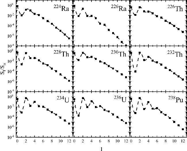
Figure 4. Angular momentum dependence of spectroscopic factors of α-decay in various actinide nuclei. The deformation parameters β2 and β3 required for the potential energy calculation are taken from table 1. |
Since the potential energy depends mainly on small deformation parameters β2 and β3, the higher multipoles in the expansion of V in (11 ) are strongly suppressed and the matrix elements in the numerator of equation (19 ) decrease rapidly for I ≥ 3. Moreover, the denominator increases with I as ~I(I + 1). These two factors account for the significant reduction of the probability to form an α-particle in the states with high angular momenta. As illustrated in figure 4, spectroscopic factors decrease substantially with I.
One notable observation is that SI exhibits a staggering pattern, with reduced probabilities of forming α-particles in states with odd I compared to neighboring states with even I. This hindrance is especially pronounced for I = 1 and becomes less significant with increasing angular momentum. The staggering behavior of SI is explained by the effect of parity splitting on Ed(I) in denominator of equation (19 ). Given that in even-even nuclei the states with negative parity and odd angular momenta are shifted up significantly compared to the states with both positive parity and even angular momentum [43], the denominator of equation (19 ) becomes larger for states with odd I, generating the staggering trend in SI for small angular momenta. As angular momentum increases, parity splitting diminishes, leading the even-odd variation in the denominator to vanish, which in turn reduces the staggering effect on SI.
The additional hindrance of the population of the α-particle in the state with angular momentum I = 1 is also related to the fact that the matrix element in equation (19 ) is significantly reduced in this case. Indeed, the first-order contribution to a1 is proportional to β1 ~ β2β3.
Using the method presented above, one can only obtain the spectroscopic factors if experimental information on B(E2) and B(E3) reduced transition probabilities is known. Although the values of B(E2) are known for most cases of interest, the information about B(E3) in actinide mass region is sparse. Therefore, the application of the model presented to the actinide nuclei where the fine structure of α-decay is measured is limited.
Since the model presented here can be used in analysis of alpha-decay fine structure, it seems relevant to consider wider range of nuclei, for which data on fine structure exist. For this, we employ the following assumption. In table 1, we present ground-state deformation parameters ${\beta }_{2}^{s}$ and ${\beta }_{3}^{s}$ obtained from [29] together with the ones extracted from experiment. We see that, in general, both sets of deformation parameters (β2, β3) and $({\beta }_{2}^{s},{\beta }_{3}^{s})$ agree well with each other. However, for some nuclei, the microscopic-macroscopic model results in ${\beta }_{3}^{s}=0$. This may be crucial for the calculation of spectroscopic factors, as zero octupole deformation leads to zero spectroscopic factors for odd angular momenta.
The reason behind this disagreement is the following. In the model presented above, the deformation parameters should be obtained with equation (18 ), i.e. from the values of B(E2) and B(E3). Meanwhile, the microscopic-macroscopic model [29] calculates deformation parameters at the minimum of the PES, yielding static deformation parameters ${\beta }_{3}^{s}$. When ${\beta }_{3}^{s}\ne 0$, the deformation parameters obtained from B(E2) and B(E3) are close to the static values as seen from the table 1. However, if ${\beta }_{3}^{s}=0$, equation (18 ) gives the dynamic deformation parameters which is related to the octupole vibrations [42]. In this case of octupole vibrations, to estimate the value β3, we assume that PES in the vicinity of ${\beta }_{3}^{s}\approx 0$ can be approximated by the oscillator (see Figure 3(a) of [44]). The energies of two lowest vibrational states in this oscillator can be associated with E(0+) and E(1-) [33, 43]. The energy interval between these two states is determined by the frequency ħω of the oscillator in β3: E(1-) ≈ ħω. The value of the dynamical deformation can be estimated as a root mean square value of β3: ${\beta }_{3}=\hslash /\sqrt{E({1}^{-}){B}_{3}}$, where B3 is the mass parameter for the motion in octupole degree of freedom. Assuming that for the given isotopic chain the mass parameter weakly depends on nuclear mass A, one can obtain 20 ), using the experimental energies of lowest 1- states in the corresponding nuclei.
$\begin{eqnarray}{\beta }_{3}(A)=\sqrt{{E}_{A-2}({1}^{-})/{E}_{A}({1}^{-})}{\beta }_{3}(A-2),\end{eqnarray}$
where EA-2(1-) and EA(1-) are the energies of lowest 1- state in the interesting nucleus and in the lighter nucleus with mass A - 2. Therefore, if microscopic-macroscopic model yields nonzero static ${\beta }_{3}^{s}$ for the nucleus with mass A - 2 and zero static ${\beta }_{3}^{s}$ for the nucleus with mass A, we can replace ${\beta }_{3}^{s}$ with an estimation β3(A) as in equation (It is clear that since ${\beta }_{3}^{s}(A-2)\ne 0$, the PES should have some degree of anharmonicity, which is neglected when oscillator approximation is considered. However, when ${\beta }_{3}^{s}(A)=0$, the static deformation ${\beta }_{3}^{s}(A-2)$ is quite small and neglecting the anharmonicity is not expected to influence the results strongly. This can be checked by direct comparison with experimental values of β3. Using equation (20 ), we obtain for dynamical deformations of 230,232Th and 234U following values: β3 = 0.094, 0.088, 0.067, respectively. These values are in good agreement with the experimental data: β3 = 0.086, 0.078, 0.077 (see table 1) with maximum deviation of ∆β3 = ± 0.01. This uncertainty in the value of β3 leads to less than two times variation in spectroscopic factors for decay into the states with odd angular momenta, while the order of magnitude is preserved. The spectroscopic factors for decay into the states with even angular momenta stay practically unchanged. Therefore, if in the cases when the experimental values of the octupole deformation β3 are not known and ${\beta }_{3}^{s}=0$, one can resort to the use of microscopic-macroscopic model predictions, with the dynamic octupole deformations estimated by the equation (20 ).
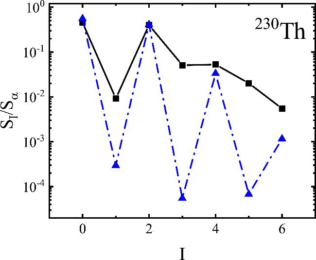
The results of the calculations of the spectroscopic factors SI with use of the deformation parameters from [29] are presented in tables 2-5 for 224-228Ra, 222-232Th, 226-236U, and 234-242Pu. If static octupole deformation in [29] is not zero ${\beta }_{3}^{s}(A)\ne 0$, the value of β3(A) is replaced by its static value: ${\beta }_{3}(A)={\beta }_{3}^{s}(A)$.However, if ${\beta }_{3}^{s}(A)=0$, the octupole deformation β3 is estimated with equation (20 ). As evident from the tables 2-5, small octupole deformation leads to an additional hindrance of spectroscopic factors for odd angular momenta I. To investigate how octupole deformation influences spectroscopic factors for even values of I we performed the calculations of spectroscopic factors in 230Th with β3 = 0.112 (black squares) and with β3 = 0.01 (blue triangles). The results are presented in figure 5. As seen, the increase of β3 leads to an increase of spectroscopic factors for both, states with odd I and to a lesser extent for states with even I ≥ 2. At the same time, the spectroscopic factor for I = 0 decreases. The reason for this is that an additional terms of potential energy in Hamiltonian (11 ) which appear due to β3 lead to the additional couplings between basis states with different I that makes the distribution of I-values wider.
Table 2. Calculated spectroscopic factors SI to form an α-particle in a state with angular momentum I and corresponding constants cI of Boltzmann distribution are presented for different Ra isotopes. The quadrupole β2 and octupole β3 deformation parameters of daughter nuclei are replaced by the ground-state deformation parameters ${\beta }_{2}^{s}$ and ${\beta }_{3}^{s}$ from [29] if ${\beta }_{2,3}^{s}\ne 0$. If ${\beta }_{3}^{s}=0$, it is replaced with the value given by the equation ( |
| 222Ra (β2 = 0.079, β3 = 0.139) | 224Ra (β2 = 0.110, β3 = 0.125) | ||||||
|---|---|---|---|---|---|---|---|
| I | E(I) (MeV) | SI | cI | I | E(I) (MeV) | SI | cI |
| 0 | 0 | 8.06 × 10⁻¹ | —— | 0 | 0 | 7.27 × 10⁻¹ | —— |
| 1 | 0.796 | 2.91 × 10⁻³ | 7.34 | 1 | 0.645 | 1.09 × 10⁻² | 7.00 |
| 2 | 0.324 | 9.27 × 10⁻² | 7.34 | 2 | 0.241 | 1.32 × 10⁻¹ | 8.39 |
| 3 | 0.84 | 7.36 × 10⁻² | 3.11 | 3 | 0.663 | 9.40 × 10⁻² | 3.57 |
| 4 | 0.653 | 1.35 × 10⁻² | 6.59 | 4 | 0.534 | 1.97 × 10⁻² | 7.36 |
| 5 | 1.026 | 8.82 × 10⁻³ | 4.61 | 5 | 0.851 | 1.21 × 10⁻² | 5.19 |
| 6 | 1.014 | 1.91 × 10⁻³ | 6.17 | 6 | 0.874 | 2.82 × 10⁻³ | 6.72 |
| | |||||||
| 226Ra (β2 = 0.110, β3 = 0.125) | 228Ra (β2 = 0.142, β3 = 0.112) | ||||||
| | |||||||
| I | E(I) (MeV) | SI | cI | I | E(I) (MeV) | SI | cI |
| | |||||||
| 0 | 0 | 6.77 × 10⁻¹ | —— | 0 | 0 | 7.06 × 10⁻¹ | —— |
| 1 | 0.6 | 1.80 × 10⁻² | 6.69 | 1 | 0.6 | 6.86 × 10⁻³ | 8.30 |
| 2 | 0.186 | 1.63 × 10⁻¹ | 9.75 | 2 | 0.136 | 2.60 × 10⁻¹ | 9.91 |
| 3 | 0.636 | 9.89 × 10⁻² | 3.64 | 3 | 0.651 | 9.73 × 10⁻³ | 7.12 |
| 4 | 0.448 | 2.43 × 10⁻² | 8.29 | 4 | 0.358 | 1.25 × 10⁻² | 12.25 |
| 5 | 0.797 | 1.40 × 10⁻² | 5.36 | 5 | 0.791 | 4.12 × 10⁻³ | 6.94 |
| 6 | 0.768 | 3.38 × 10⁻³ | 7.41 | 6 | 0.641 | 4.53 × 10⁻⁴ | 12.01 |
Figure 5. Angular momentum dependence of spectroscopic factors of α-decay in 230Th. The calculations performed with the deformation parameters β20 = 0.174 and β3 = 0.112 (see table 3) are shown by black squares connected by solid line. The calculations performed with β20 = 0.174 and β3 = 0.01 are shown by triangles connected by dashed line. |
It is interesting to compare the observed trend of SI with the prescription provided by the empirical BD approach. To do so, we assume that the calculated spectroscopic factors are presented as ${S}_{I}=\exp \left(-{c}_{I}E(I)\right)$, where E(I) is the excitation energy of the yrast state with angular momentum I in the daughter nucleus. The resulting values of cI are presented in tables 2-5. First, it is evident that cI is not a constant but varies within a large interval between ~5 MeV-1 and ~20 MeV-1 for different nuclei and for different angular momenta of the same nucleus. This dependence is determined not only by the energies of the excited states of the daughter nucleus, as is suggested by the Boltzmann distribution, but also by its quadrupole and octupole deformation parameters (see equation (19 )).
With a closer look at the data presented in tables 2-5, it becomes apparent that the values of ceven-I are significantly impacted by the quadrupole deformation, while codd-I is influenced by the octupole deformation of the daughter nucleus. Notably, a considerable quadrupole deformation of the daughter nucleus β2 ≥ 0.15 requires the use of BD description with values cI around (15-20) MeV-1. In contrast, for nuclei with smaller quadrupole deformation, the cI ≈ (5-8) MeV-1 is required. The values of codd-I>1 vary in the interval ~(5-9) MeV-1 for all considered cases. The strongest variation is observed for the values c1 determining the BD spectroscopic factor for I = 1. Depending on quadrupole β2 and octupole β3 deformations of daughter nucleus as well as on the excitation energy of the lowest negative parity state E(1-), the values of c1 vary in the interval ~(5-26) MeV-1.
Table 3. The same as in table 2, but for Th isotopes. |
| 222Th (β2 = 0.078, β3 = 0.125) | 224Th (β2 = 0.111, β3 = 0.127) | ||||||
|---|---|---|---|---|---|---|---|
| I | E(I) (MeV) | SI | cI | I | E(I) (MeV) | SI | cI |
| 0 | 0 | 9.11 × 10⁻¹ | —— | 0 | 0 | 7.14 × 10⁻¹ | —— |
| 1 | 0.853 | 7.83 × 10⁻⁴ | 8.39 | 1 | 0.412 | 1.89 × 10⁻⁴ | 20.81 |
| 2 | 0.389 | 5.50 × 10⁻² | 7.46 | 2 | 0.178 | 2.08 × 10⁻¹ | 8.82 |
| 3 | 0.793 | 2.72 × 10⁻² | 4.55 | 3 | 0.474 | 4.80 × 10⁻² | 6.40 |
| 4 | 0.741 | 2.62 × 10⁻³ | 8.02 | 4 | 0.41 | 1.55 × 10⁻² | 10.17 |
| 5 | 1.038 | 2.75 × 10⁻³ | 5.68 | 5 | 0.634 | 1.14 × 10⁻² | 7.05 |
| 6 | 1.122 | 3.97 × 10⁻⁴ | 6.98 | 6 | 0.688 | 1.87 × 10⁻³ | 9.13 |
| | |||||||
| 226Th (β2 = 0.122, β3 = 0.141) | 228Th (β2 = 0.143, β3 = 0.139) | ||||||
| | |||||||
| I | E(I) (MeV) | SI | cI | I | E(I) (MeV) | SI | cI |
| | |||||||
| 0 | 0 | 5.30 × 10⁻¹ | —— | 0 | 0 | 4.96 × 10⁻¹ | —— |
| 1 | 0.242 | 2.14 × 10⁻² | 15.88 | 1 | 0.215 | 1.63 × 10⁻² | 19.14 |
| 2 | 0.111 | 2.94 × 10⁻¹ | 11.02 | 2 | 0.084 | 3.36 × 10⁻¹ | 12.98 |
| 3 | 0.317 | 8.68 × 10⁻² | 7.71 | 3 | 0.29 | 7.60 × 10⁻² | 8.89 |
| 4 | 0.301 | 3.67 × 10⁻² | 10.98 | 4 | 0.25 | 4.31 × 10⁻² | 12.58 |
| 5 | 0.473 | 2.27 × 10⁻² | 8.01 | 5 | 0.433 | 2.37 × 10⁻² | 8.64 |
| 6 | 0.549 | 5.20 × 10⁻³ | 9.58 | 6 | 0.479 | 5.63 × 10⁻³ | 10.81 |
| | |||||||
| 230Th (β2 = 0.164, β3 = 0.112) | 232Th (β2 = 0.174, β3 = 0.083) | ||||||
| | |||||||
| I | E(I) (MeV) | SI | cI | I | E(I) (MeV) | SI | cI |
| | |||||||
| 0 | 0 | 4.56 × 10⁻¹ | —— | 0 | 0 | 4.92 × 10⁻¹ | —— |
| 1 | 0.253 | 9.17 × 10⁻³ | 18.54 | 1 | 0.474 | 1.38 × 10⁻⁴ | 18.75 |
| 2 | 0.067 | 4.02 × 10⁻¹ | 13.59 | 2 | 0.063 | 4.31 × 10⁻¹ | 13.35 |
| 3 | 0.321 | 5.07 × 10⁻² | 9.29 | 3 | 0.538 | 1.59 × 10⁻² | 7.70 |
| 4 | 0.211 | 5.27 × 10⁻² | 13.95 | 4 | 0.205 | 4.73 × 10⁻² | 14.88 |
| 5 | 0.446 | 2.01 × 10⁻² | 8.76 | 5 | 0.656 | 8.71 × 10⁻³ | 7.23 |
| 6 | 0.416 | 5.49 × 10⁻³ | 12.51 | 6 | 0.412 | 3.24 × 10⁻³ | 13.91 |
Table 4. The same as in table 2, but for U isotopes. |
| 226U (β2 = 0.111, β3 = 0.140) | 228U (β2 = 0.144, β3 = 0.153) | ||||||
|---|---|---|---|---|---|---|---|
| I | E(I) (MeV) | SI | cI | I | E(I) (MeV) | SI | cI |
| 0 | 0 | 6.18 × 10⁻¹ | —— | 0 | 0 | 3.58 × 10⁻¹ | —— |
| 1 | 0.246 | 1.78 × 10⁻² | 16.39 | 1 | 0.251 | 6.22 × 10⁻² | 11.06 |
| 2 | 0.183 | 2.39 × 10⁻¹ | 7.83 | 2 | 0.098 | 3.43 × 10⁻¹ | 10.92 |
| 3 | 0.467 | 7.63 × 10⁻² | 5.51 | 3 | 0.305 | 1.17 × 10⁻¹ | 7.05 |
| 4 | 0.439 | 2.65 × 10⁻² | 8.27 | 4 | 0.284 | 6.60 × 10⁻² | 9.57 |
| 5 | 0.65 | 1.71 × 10⁻² | 6.26 | 5 | 0.465 | 3.61 × 10⁻² | 7.14 |
| 6 | 0.749 | 3.68 × 10⁻³ | 7.48 | 6 | 0.535 | 1.09 × 10⁻² | 8.45 |
| | |||||||
| 230U (β2 = 0.154, β3 = 0.139) | 232U (β2 = 0.174, β3 = 0.111) | ||||||
| | |||||||
| I | E(I) (MeV) | SI | cI | I | E(I) (MeV) | SI | cI |
| | |||||||
| 0 | 0 | 3.55 × 10⁻¹ | —— | 0 | 0 | 4.09 × 10⁻¹ | —— |
| 1 | 0.23 | 5.42 × 10⁻² | 12.68 | 1 | 0.328 | 1.34 × 10⁻² | 13.15 |
| 2 | 0.072 | 3.73 × 10⁻¹ | 13.68 | 2 | 0.058 | 4.28 × 10⁻¹ | 14.63 |
| 3 | 0.308 | 9.86 × 10⁻² | 7.52 | 3 | 0.396 | 5.10 × 10⁻² | 7.52 |
| 4 | 0.226 | 6.98 × 10⁻² | 11.78 | 4 | 0.187 | 6.52 × 10⁻² | 14.60 |
| 5 | 0.451 | 3.29 × 10⁻² | 7.57 | 5 | 0.519 | 2.17 × 10⁻² | 7.38 |
| 6 | 0.447 | 1.03 × 10⁻² | 10.24 | 6 | 0.378 | 7.17 × 10⁻³ | 13.06 |
| | |||||||
| 234U (β2 = 0.195, β3 = 0.094) | 236U (β2 = 0.205, β3 = 0.088) | ||||||
| | |||||||
| I | E(I) (MeV) | SI | cI | I | E(I) (MeV) | SI | cI |
| | |||||||
| 0 | 0 | 3.49 × 10⁻¹ | —— | 0 | 0 | 4.00 × 10⁻¹ | —— |
| 1 | 0.508 | 1.11 × 10⁻³ | 13.39 | 1 | 0.714 | 8.12 × 10⁻⁵ | 13.19 |
| 2 | 0.053 | 5.00 × 10⁻¹ | 13.06 | 2 | 0.049 | 4.91 × 10⁻¹ | 14.52 |
| 3 | 0.572 | 1.94 × 10⁻² | 6.90 | 3 | 0.774 | 1.20 × 10⁻² | 5.72 |
| 4 | 0.174 | 9.87 × 10⁻² | 13.31 | 4 | 0.162 | 7.82 × 10⁻² | 15.73 |
| 5 | 0.687 | 1.54 × 10⁻² | 6.07 | 5 | 0.884 | 9.74 × 10⁻³ | 5.24 |
| 6 | 0.357 | 1.08 × 10⁻² | 12.67 | 6 | 0.333 | 6.88 × 10⁻³ | 14.95 |
Table 5. The same as in table 2 but for Pu isotopes. |
| 234Pu (β2 = 0.185, β3 = 0.098) | 236Pu (β2 = 0.206, β3 = 0.079) | ||||||
|---|---|---|---|---|---|---|---|
| I | E(I) (MeV) | SI | cI | I | E(I) (MeV) | SI | cI |
| 0 | 0 | 4.93 × 10⁻¹ | —— | 0 | 0 | 4.70 × 10⁻¹ | —— |
| 1 | 0.367 | 6.11 × 10⁻⁵ | 26.44 | 1 | 0.563 | 8.59 × 10⁻⁴ | 12.54 |
| 2 | 0.051 | 4.36 × 10⁻¹ | 16.29 | 2 | 0.048 | 4.72 × 10⁻¹ | 15.64 |
| 3 | 0.435 | 1.86 × 10⁻² | 9.16 | 3 | 0.629 | 3.97 × 10⁻³ | 8.79 |
| 4 | 0.169 | 4.07 × 10⁻² | 18.94 | 4 | 0.157 | 4.73 × 10⁻² | 19.44 |
| 5 | 0.558 | 8.47 × 10⁻³ | 8.55 | 5 | 0.747 | 3.15 × 10⁻³ | 7.71 |
| 6 | 0.347 | 2.16 × 10⁻³ | 17.69 | 6 | 0.323 | 2.04 × 10⁻³ | 19.17 |
| | |||||||
| 238Pu (β2 = 0.215, β3 = 0.067) | 240Pu (β2 = 0.226, β3 = 0.084) | ||||||
| | |||||||
| I | E(I) (MeV) | SI | cI | I | E(I) (MeV) | SI | cI |
| | |||||||
| 0 | 0 | 4.49 × 10⁻¹ | —— | 0 | 0 | 4.24 × 10⁻¹ | —— |
| 1 | 0.786 | 6.03 × 10⁻⁴ | 9.43 | 1 | 0.688 | 5.21 × 10⁻⁴ | 10.99 |
| 2 | 0.043 | 4.87 × 10⁻¹ | 16.73 | 2 | 0.045 | 4.97 × 10⁻¹ | 15.55 |
| 3 | 0.849 | 3.14 × 10⁻³ | 6.79 | 3 | 0.744 | 6.12 × 10⁻³ | 6.85 |
| 4 | 0.143 | 5.40 × 10⁻² | 20.41 | 4 | 0.149 | 6.28 × 10⁻² | 18.58 |
| 5 | 0.962 | 2.92 × 10⁻³ | 6.07 | 5 | 0.848 | 5.59 × 10⁻³ | 6.12 |
| 6 | 0.296 | 2.54 × 10⁻³ | 20.19 | 6 | 0.31 | 3.60 × 10⁻³ | 18.15 |
| | |||||||
| 242Pu (β2 = 0.236, β3 = 0.084) | |||||||
| | |||||||
| I | E(I) (MeV) | SI | cI | ||||
| | |||||||
| 0 | 0 | 4.09 × 10⁻¹ | —— | ||||
| 1 | 0.68 | 4.08 × 10⁻⁴ | 11.48 | ||||
| 2 | 0.045 | 5.05 × 10⁻¹ | 15.19 | ||||
| 3 | 0.732 | 6.29 × 10⁻³ | 6.92 | ||||
| 4 | 0.148 | 6.85 × 10⁻² | 18.12 | ||||
| 5 | 0.827 | 5.94 × 10⁻³ | 6.20 | ||||
| 6 | 0.307 | 4.18 × 10⁻³ | 17.84 | ||||
It is seen that in the cases where the energies of the daughter nucleus E(I = 1) are relatively small (less than 500 keV), the description of the spectroscopic factors S1 with BD requires especially large values of c1, compared to other odd angular momentum states. Qualitatively, this can be understood as follows. BD assumes that the probability to populate the system in the certain basis state ${P}_{I}(\cos \varepsilon )$ exponentially depends on the diagonal matrix element of the Hamiltonian (11 ): 21 ) becomes more accurate. However, for small I, the potential energy contribution cannot be neglected. Indeed, Legendre polynomials are peaked at ε = 0 with a width 1/I. Therefore, for small I, a significant part of the wave function of the basis state ${P}_{I}(\cos \varepsilon )$ lies in the region where the potential energy is large. This contribution leads to the additional suppression of SI for small I, which is reflected in the larger values of c1 comparing to other angular momenta. This effect is especially pronounced when the energy E(I = 1) is small and the role of the potential energy term in the matrix element (21 ) increases.
$\begin{eqnarray}\begin{array}{rcl}{H}_{I} & = & \frac{2I+1}{2}\langle {P}_{I}(\cos \varepsilon )| H| {P}_{I}(\cos \varepsilon )\rangle ,\\ {S}_{I} & \sim & \exp (-\tilde{c}{H}_{I}).\end{array}\end{eqnarray}$
This matrix element consists of the kinetic energy part $E(I)+\frac{{\hslash }^{2}I(I+1)}{2{\Im }_{R}}$ and the potential energy part $\frac{2I+1}{2}\langle {P}_{I}(\cos \varepsilon )| V(R(\varepsilon ),\varepsilon )| {P}_{I}(\cos \varepsilon )\rangle $. Neglecting the contribution of the potential energy and assuming that E(I) ~ I(I + 1), we obtain the conventional expression for BD: $\begin{eqnarray}{S}_{I}\sim \exp (-cE(I)),\end{eqnarray}$
with c being almost independent of I. Note that as I increases, the kinetic energy term increases as well and neglecting the potential energy part of the matrix element (4. Summary
Based on the DNS concept, we propose a method to calculate the angular momentum dependence of spectroscopic factor for α-decay of heavy nuclei. The method is based on the assumption that prior to tunneling of the α-particle through the outer barrier, the parent nucleus can be modeled as an α-DNS.
Solving the Schrodinger equation for collective angular motion, we determine the probabilities to find an α-DNS in the state where both the daughter nucleus and the relative rotation of the DNS have a given angular momentum I. The spectroscopic factors are found to be strongly dependent on the quadrupole and octupole deformations of the daughter nucleus. If the daughter nucleus is almost spherical, it is predominantly populated in the state I = 0, while the population of states with all other values of I is strongly suppressed. If the daughter nucleus possesses the quadrupole deformation but a negligible octupole deformation, the states with even angular momenta are primarily populated. To populate the states with odd angular momenta, the daughter nucleus should be octupole deformed. The spectroscopic factors are calculated for 224-228Ra, 222-232Th, 226-236U, and 234-242Pu which are of interest for the analysis of experimental information of α-decay fine structure. The calculation was performed with the static values of quadrupole and octupole deformation parameters obtained from [29]. If static value of octupole deformation is zero, it was replaced with an approximate value, obtained with use of the experimental energies of lowest 1- states in the nucleus of interest and neighboring nucleus. The results presented might be useful in the analysis of the alpha-decay fine-structure in the actinide mass region.