


1. Introduction
Presently, one of the most popular and successful approaches to many quantum many-body systems is the density functional theory (DFT), rooted in the Hohenberg-Kohn theorem [1]. Especially, for nuclear systems with strong spin-orbital coupling, the relativistic density functional theory (RDFT) that takes into account the Lorentz symmetry at the very beginning has achieved great success in describing the ground state properties of almost all nuclei on the nuclide chart [2-12]. Although technically more complicated, there are several essential advantages compared to the non-relativistic density functionals [2, 13, 14]: automatically giving the spin degree of freedom and the large spin-orbital potentials; providing the relativistic saturation mechanism; natural explanation of hidden pseudo-spin symmetry in nuclear single-particle spectrum [15-17]; discovery of spin symmetry for anti-nucleon [17, 18]; success of relativistic Brueckner calculations [10, 19]; self-consistent treatment of time-odd fields important for nuclear properties associated with rotation [5, 7].
To date, most practical DFT applications were performed with the Kohn-Sham scheme [2]. Thus, the essential part of RDFT is to solve the corresponding Kohn-Sham equations, i.e., the Dirac equations of nucleons. One can solve the Dirac equations either in basis expansion method like harmonic oscillator [7, 20, 21], Schrödinger Woods-Saxon (WS) [22] and Dirac WS [22, 23] bases or directly in the coordinate space like the shooting method [24, 25], the finite element method [25-27], the Green's function method [28-30] and the imaginary time method [31]. In contrast to the former method that may be limited on the basis space, the latter one would be more efficient for nuclear phenomena with large spatial distributions such as halo phenomena or nuclear fissions [4]. It should be noted that solving the Dirac equation in the coordinate space may face the well-known variational collapse [31] and Fermion doubling [32, 33] problems. Up to now, in literature, the inverse Hamiltonian method [33, 34] and the preconditioned conjugate gradient method with a filtering function [35, 36] have been used to overcome the variational collapse problem, while the Wilson term [33], the Fourier spectral method [34-36] and the asymmetric difference formula [37] to overcome the Fermion doubling problem.
On the other hand, with the great improvement of computer hardware and the rapid development of various algorithms, artificial intelligence nowadays has a profound impact on basic scientific research. In nuclear physics, various machine learning (ML) algorithms have been utilized to solve many practical problems and achieved remarkable successes, for recent reviews, see [38-40].
The ML algorithms are mainly divided into three categories: supervised learning, unsupervised learning and reinforcement learning. Notably, the unsupervised learning algorithms have received extensive attention in scientific research mainly due to their independence of available labeled data. For instance, aiming to attack the nuclear many-body problems, Keeble and Rios used the artificial neural networks to determine the deuteron wave function [41]; Adams et al performed variational Monte Carlo calculations with artificial neural networks for light nuclei [42, 43]; Yang and Zhao developed the FeynmanNet which reaches a high accuracy of nuclear ground-state energy in a variational way and scales polynomially with the number of nucleons [44].
In fact, the ML algorithms have been applied to directly solve the differential equations in quantum mechanics. In 1997, Lagaris et al used a single-hidden-layer neural network (NN) to solve the Schrödinger and Dirac equations of μ atoms [45]. Later, Jin et al used NNs to solve the ground state and excited states of the Schrödinger equation in the harmonic oscillator potential [46, 47]. Pu et al used a deep NN to represent the cumulative distribution function which can avoid integral operations, and solved the ground state of the Schrödinger equation [48]. Most recently, applying the inverse Hamiltonian method to avoid variational collapse and invoking the variational principle, Wang et al successfully solved the Dirac equation in Coulomb and WS potentials by using a deep neural network approach [49].
In recent years, physics-informed neural networks (PINNs) have emerged as novel ML tools, arousing great interest of researchers [50]. The PINNs are neural networks that encode the model equations into the neural network itself and have been used to solve various differential equations due to the prominent characteristics [51-54]: incorporating physical laws and domain-specific knowledge to enhance predictive capabilities, the ability to learn from sparse data input, meshless alternative to classical methods, opening up new avenues for solving inverse problems. The PINN has been extensively applied to solve ordinary and partial differential equations in fluid dynamics, material science, quantum mechanics, and so on [51-55]. Indeed, the method in [45] can be also regarded as the early PINN [53]. Therefore, it is believed that the PINN can be used to solve the nuclear Dirac equation. More importantly, the PINN employs the residual of the Dirac equation as the objective function rather than the variation of energy expectation value, so that the well-known variational collapse problem [31] can be naturally avoided. It is easy to know, if the residual equals to zero, the wave functions G(r) and F(r) automatically satisfy the Dirac equation exactly, i.e., the eigen solutions are obtained. Furthermore, by calculating the derivatives with automatic differentiation (AD) techniques [56-58], the PINN can overcome the Fermion doubling problem as well.
In this paper, a PINN will be constructed for the first time to solve the nuclear Dirac WS potential [59]. To test the performance of the PINN, the energies and wave functions of neutron orbitals below the Fermi surface for 16O and 208Pb thus obtained are compared with those obtained by the traditional shooting method. In section 2 , the theoretical framework including the Dirac equation and the PINN methodology is briefly introduced. In section 3 , numerical details are given, and in section 4 , results and discussions are presented. Finally, a summary is given in section 5 .
2. Theoretical framework
2.1. Dirac equation
In the framework of the relativistic density functional theory, instead of the Schrödinger equation, the nucleus is described as a system of Dirac nucleons that satisfy the following Dirac equation [2]
$\begin{eqnarray}\left[{\boldsymbol{\alpha }}\cdot ({\boldsymbol{p}}-{\boldsymbol{V}})+{V}^{0}+\beta (M+S)\right]{\psi }_{i}({\boldsymbol{r}})={\epsilon }_{i}{\psi }_{i}({\boldsymbol{r}}),\end{eqnarray}$
where p and M are the nucleon momentum and mass, (V0(r), V(r)) is the repulsive vector field and S(r) is the attractive scalar field, εi and ψi(r) are eigen energy and wave function of the single-particle state i, respectively.In the case of spherical symmetry, equation (1 ) can be reduced as the radial equation, which depends only on the radial coordinate r. As for now, the wave function ψi(r) is characterized by the radial quantum number n, the angular momentum quantum numbers l, j and m, as well as the parity, which can be formulated as 2 ), one can obtain the corresponding radial Dirac equations
$\begin{eqnarray}{\psi }_{n\kappa m}({\boldsymbol{r}},s)=\frac{1}{r}\left(\begin{array}{c}{\rm{i}}{G}_{n\kappa }(r){Y}_{jm}^{l}(\theta ,\phi ,s)\\ -{F}_{n\kappa }(r){Y}_{jm}^{\tilde{l}}(\theta ,\phi ,s)\end{array}\right),\end{eqnarray}$
where κ = (-1)j+l+1/2(j + 1/2) is the relativistic quantum number, G(r) and F(r) are the large and small components of the wave function, ${Y}_{jm}^{l}$ and ${Y}_{jm}^{\tilde{l}}$ are the spinor spherical harmonics with $l=j+\frac{1}{2}{\rm{sgn}}(\kappa )$ and $\tilde{l}=j-\frac{1}{2}{\rm{sgn}}(\kappa )$, respectively. The radial wave functions with the same quantum number κ but different quantum number n are orthogonal, thus the Dirac equation can be resolved with different κ blocks. With wave function ( $\begin{eqnarray}\begin{array}{l}\left(\frac{{\rm{d}}}{{\rm{d}}r}-\frac{\kappa }{r}\right){F}_{n\kappa }(r)+[{E}_{n\kappa }-U(r)]{G}_{n\kappa }(r)=0,\\ \left(\frac{{\rm{d}}}{{\rm{d}}r}+\frac{\kappa }{r}\right){G}_{n\kappa }(r)-[{E}_{n\kappa }+2M-W(r)]{F}_{n\kappa }(r)=0,\end{array}\end{eqnarray}$
where U(r) = V(r) + S(r), W(r) = V(r) - S(r) and Enκ = εnκ - M.For the potentials, Koepf and Ring have shown that the smooth WS shaped potentials can approximate the self-consistently determined relativistic scalar- and vector-potentials without changing the resulting single-particle spectra below the Fermi surface [59]. For the neutron, the WS shaped potentials are written as
$\begin{eqnarray}\begin{array}{rcl}{U}_{{n}} & = & \frac{{V}_{{n}}^{0}}{1+{{\rm{e}}}^{(r-{R}_{{n}})/{a}_{{n}}}},\\ {W}_{{n}} & = & \frac{-{\lambda }_{{n}}{V}_{{n}}^{0}}{1+{{\rm{e}}}^{(r-{R}_{{n}}^{ls})/{a}_{{n}}^{ls}}},\end{array}\end{eqnarray}$
with ${V}_{{n}}^{0}=V\left(1-{\kappa }_{{\rm{WS}}}\frac{N-Z}{N+Z}\right)$, ${R}_{{n}}={r}_{0}^{{n}}{A}^{\frac{1}{3}}$ and ${R}_{{n}}^{ls}={r}_{0}^{ls,{n}}{A}^{\frac{1}{3}}$, where the parameters V = -71.28 MeV, κWS = 0.462, ${\lambda }_{{n}}=11.12,{r}_{0}^{{n}}=1.233\,{\rm{fm}}$, an = 0.615 fm, ${r}_{0}^{ls,{n}}=1.144\,{\rm{fm}}$ and ${a}_{{n}}^{ls}=0.648\,{\rm{fm}}$ [59].2.2. Physics-informed neural network
The starting point of the PINN is using a neural network N(θ) (here θ denotes all the NN parameters) to approximate the solution of a differential equation, according to the universal approximation theorem [60, 61]. For instance, here we can use NN to approximate the eigen wave functions Gnκ(r) and Fnκ(r) of the radial Dirac equations (3 ). Then, one can calculate the derivatives of the NN's outputs with respect to the inputs by the automatic differentiation [56], and results in the representation of the residual of the differential equation, i.e., the so-called physics-informed neural network. To find the final solutions of the differential equation, the loss function ${ \mathcal L }(\theta )$ is constructed as a weighted sum of the residual of the differential equation ${{ \mathcal L }}_{{\rm{DE}}}$, the residual of the boundary/initial condition ${{ \mathcal L }}_{{\rm{BI}}}$ and/or the deviations from the available data ${{ \mathcal L }}_{{\rm{data}}}$:
$\begin{eqnarray}{ \mathcal L }(\theta )={\omega }_{{\rm{DE}}}{{ \mathcal L }}_{{\rm{DE}}}(\theta )+{\omega }_{{\rm{BI}}}{{ \mathcal L }}_{{\rm{BI}}}(\theta )+{\omega }_{{\rm{data}}}{{ \mathcal L }}_{{\rm{data}}}(\theta ).\end{eqnarray}$
Finally, the differential equation is solved by minimizing the loss function ${ \mathcal L }(\theta )$ with optimization algorithms such as the gradient descent method.In this work, in order to explicitly consider the asymptotic behaviors of the bound states at r = 0 and r = ∞, the wave functions Gnκ(r) and Fnκ(r) are parametrized as [45]5 ) are exactly: ωDE = 1.0, ωBI = 0.0 and ωdata = 0.0. In this sense, our PINN framework is actually an unsupervised method.
$\begin{eqnarray}\left(\begin{array}{c}{G}_{n\kappa }(r)\\ {F}_{n\kappa }(r)\end{array}\right)\approx r{{\rm{e}}}^{-\beta r}N(r,\theta ),\end{eqnarray}$
where β > 0 is a trainable parameter and N(r, θ) is a neural network. The input of N(r, θ) is the one-dimensional radial coordinate r, and the output is a vector with two components. With the embedding of the boundary conditions in the NN and no available data being introduced, the weights in equation (With the AD, the derivatives in the radial Dirac equations (3 ) can be calculated, thus lead to the residuals of the radial Dirac equations:
$\begin{eqnarray}\begin{array}{rcl}{f}_{1} & := & \left(\frac{{\rm{d}}}{{\rm{d}}r}-\frac{\kappa }{r}\right)F(r)+[E-U(r)]G(r),\\ {f}_{2} & := & \left(\frac{{\rm{d}}}{{\rm{d}}r}+\frac{\kappa }{r}\right)G(r)-[E+2M-W(r)]F(r),\end{array}\end{eqnarray}$
where $f(r,\theta ,\beta ,E)={({f}_{1},{f}_{2})}^{T}$ is regarded as the physics-informed neural network, and the energy E is a trainable parameter the same as θ and β. As a powerful tool, the AD uses exact expressions with floating-point values rather than expression strings as in the symbolic differentiation which makes it memory-efficient and involves no approximation error as in numerical differentiation [57, 58]. Also thanks to this characteristic, the Fermion doubling problem in the Dirac equation [32, 33] can be addressed by using the AD technique.With the PINN (7 ), the radial Dirac equations (3 ) are solved by minimizing the following loss function, 7 ) evaluated at the collocation points ${\{{r}_{f}^{i}\}}_{i=1}^{{N}_{f}}$. If the ${{ \mathcal L }}_{{\rm{DE}}}$ equals to zero, the wave functions G(r) and F(r) satisfy the radial Dirac equations (3 ) exactly, i.e., the eigen solutions. The term ${{ \mathcal L }}_{{\rm{conz}}}$ is a constraint to avoid the trivial zero solutions by restricting the maximum of the wave function G(r) at the collocation points to 1. The term ${{ \mathcal L }}_{{\rm{orth}}}$ is applied to search the excited states, which requires the current wave functions G(r) and F(r) to be orthogonal to the sum of the solved wave functions Gsum(r) and Fsum(r) [47]. The wave functions are normalized in the final step after being solved by the PINN.
$\begin{eqnarray}{ \mathcal L }(\theta ,\beta ,E)={{ \mathcal L }}_{{\rm{DE}}}+{{ \mathcal L }}_{{\rm{conz}}}+{{ \mathcal L }}_{{\rm{orth}}},\end{eqnarray}$
where $\begin{eqnarray}\begin{array}{rcl}{{ \mathcal L }}_{{\rm{DE}}} & = & \frac{1}{{N}_{f}}\displaystyle \sum _{i=1}^{{N}_{f}}\left[| {f}_{1}({r}_{f}^{i}){| }^{2}+| {f}_{2}({r}_{f}^{i}){| }^{2}\right],\\ {{ \mathcal L }}_{{\rm{conz}}} & = & {\left[{G}_{{\rm{\max }}}({r}_{f}^{i})-1\right]}^{2},\\ {{ \mathcal L }}_{{\rm{orth}}} & = & {\int }_{0}^{{r}_{\max }}\left[{G}_{{\rm{sum}}}(r)G(r)+{F}_{{\rm{sum}}}(r)F(r)\right]{\rm{d}}r.\end{array}\end{eqnarray}$
Here, the term ${{ \mathcal L }}_{{\rm{DE}}}$ is the mean square error of equation (3. Numerical details
Here, the PINN approach is established for solving the Dirac equation with a given mean field potential like equation (4 ). As examples, all the neutron orbitals below the Fermi surface will be solved for a light nucleus 16O and a heavy nucleus 208Pb. In order to assess its performance, the eigen energies and wave functions thus obtained will be compared with the conventional shooting method [62]. Noted that it has been shown in literature that in calculating the single-particle energies the consistency between the shooting method and other numerical methods, such as the Green's function method [28], the preconditioned conjugate gradient method with a filtering function [35] and the five-point asymmetric finite difference method [37], is at least 10-3 MeV. Here, the results from the shooting method are used as a benchmark.
For the PINN construction, a fully-connected neural network is used to express the N(r, θ) in wave functions equation (6 ). The Sigmoid activation function is adopted for hidden layers. The weights of the NN are initialized with the Xavier normal distribution and the biases are initialized as 0, which are the same recipe as adopted in the original PINN [50, 63]. For other trainable parameters, the parameter β is initialized as 1.0 fm-1, and the energy E is initialized as -60.0 MeV which is close to the bottom of Fermi sea in the Dirac WS potential. First, to choose an appropriate NN architecture, we calculated the 1s1/2 orbital of 208Pb under various combinations of the number of hidden layers Nlay and the number of neurons per layer Nneu as an example. For the training of NN, a sufficient number of iterations, 80000 epochs, are used to ensure high precision. The other numerical details are the same for different NN architectures. Table 1 shows the RMS errors of the wave functions G(r) obtained by PINN with respect to the shooting method, which are evaluated on the 200 uniform mesh points in the range of (0.0, 20.0] fm. It can be seen that as Nlay or Nneu increases, the RMS error generally shows a decreasing trend, with the increase in Nlay demonstrating a more pronounced effect. In this test, the NN with Nlay = 3 and Nneu = 80 achieved the smallest RMS error and was consequently selected as the architecture for subsequent calculations.
Table 1. The impact of NN architectures on the accuracy of the PINN. Taking the 1s1/2 orbital of 208Pb as an example, we show the root-mean-square (RMS) errors of the wave functions G(r) obtained by PINN with respect to the shooting method, which are evaluated on the 200 uniform mesh points in the range of (0.0, 20.0] fm. |
| Nlay\Nneu | 10 | 20 | 40 | 80 | 100 |
|---|---|---|---|---|---|
| 1 | 0.019468 | 0.020548 | 0.015200 | 0.012666 | 0.014222 |
| 2 | 0.005728 | 0.000322 | 0.000266 | 0.000236 | 0.000109 |
| 3 | 0.000141 | 0.000522 | 0.000055 | 0.000051 | 0.000070 |
| 4 | 0.000112 | 0.000083 | 0.000574 | 0.000060 | 0.000073 |
For the evaluation of loss function (8 ), the collocation points ${\{{r}_{f}^{i}\}}_{i=1}^{{N}_{f}}$ are selected in a range of (0.0, 20.0] fm. The residual-based adaptive refinement is used to improve the distribution of the collocation points and the performance of the PINN [64]. In practice, we adopt an initial set of 200 mesh points with an equal interval of ∆r = 0.1 fm. Every 2000 epochs, 10 new collocation points corresponding to the largest residuals are added to the set. The total number of collocation points in the set is capped at 400.
The loss function is minimized by the Adam optimizer [65]. A preliminary learning rate is set as 10-3. The mean values of the losses within 2000 epochs, denoted as Lmean, are calculated. A conditional threshold ε = 5 × 10⁻⁵ is then set. If Lmean drops below the threshold ε, a learning rate scheduler is employed to enhance the accuracy of the PINN. Specifically, the learning rate is multiplied by a factor of $\gamma$ = 0.8 every 1000 epochs, and this adjustment process is carried out for a maximum of 20 times.
4. Results and discussion
4.1. Light nucleus 16O
The light nucleus 16O has eight protons and eight neutrons, and its ground state is spherical. There are only three single-particle orbitals below the proton or neutron Fermi surface, namely 1s1/2, 1p3/2 and 1p1/2, which are occupied by 2, 4 and 2 nucleons respectively. Therefore, in the solution of PINN, only the lowest energy level in each of their respective κ blocks needs to be solved, which also means that the third term ${{ \mathcal L }}_{{\rm{orth}}}$ in the loss function (8 ) does not need to be introduced.
Figure 1 shows the losses and the energies varying with epochs for the three neutron orbitals 1s1/2, 1p3/2 and 1p1/2 of 16O. As seen in figure 1(a), all the three curves of losses basically decrease with the increasing epoch although many irregular peaks emerged during the optimization. After closely analyzing the relationship between the loss and energy changes, we found that when the loss exhibits irregular peaks, the energy values simultaneously appear as small fluctuations (about 10-3 MeV). Therefore, it is inferred that both the energy and wave functions contribute to these peaks, which is the natural consequence in solving the Dirac equation. After 16818, 36138 and 41499 epochs, respectively, the mean values of the losses decrease below the conditional threshold ε for 1s1/2, 1p3/2 and 1p1/2. Finally, after further optimization, the loss for each orbital decreases to the level of 10-6 or even below, which means that a PINN solution with high precision to the Dirac equation has been achieved. The lowest final loss 2.52 × 10⁻⁷ is obtained for the 1p3/2 orbital. After comparing the different contributions to the loss, it is found that the ${{ \mathcal L }}_{{\rm{DE}}}$ term in equation (8 ), i.e., the residuals of the Dirac equations, contribute most to the final loss. As seen in figure 1(b), starting from the same initial value -60 MeV, the single-particle energies of the three orbitals gradually converge to the exact eigenvalues with the increasing epoch. Comparing the curves in figures 1(a) and (b), the energies vary continuously during the sharp decrease of the losses and converge to the eigenvalues when the losses steadily approach zero. Noted that, when the mean value of the losses reaches the threshold ε, the energy has also approached the eigenvalue very closely. Because the eigenvalue of the 1s1/2 orbital is closer to the initial value of the energy, the loss and energy of the 1s1/2 orbital converge the fastest.
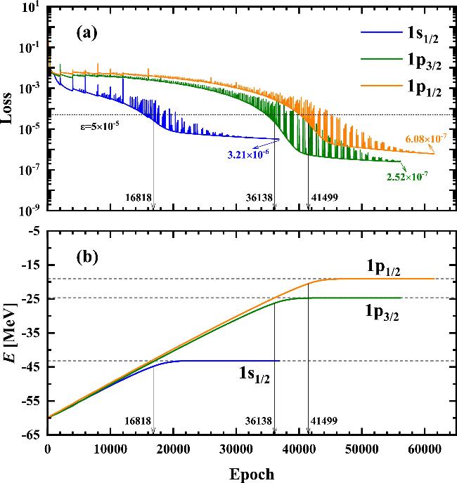
Figure 1. The losses (a) and the energies (b) as functions of epochs, for the neutron orbitals 1s1/2 (blue), 1p3/2 (green), and 1p1/2 (orange) of 16O in the Dirac WS potential. The dashed lines in (b) are the values obtained by the shooting method. |
Figure 2 shows the obtained wave functions by the PINN, in comparison with the results by the shooting method. Here, the box size Rbox = 20.0 fm and step size ∆r = 0.1 fm are used, which can guarantee the solution's accuracy of the shooting method. As seen in figures 2(a)-(c), the wave functions of all the three orbitals obtained by the PINN are consistent with those by the shooting method. Figures 2(d)-(f) show the differences of the obtained wave functions between the PINN and the shooting method. It can be seen that the maximum deviations ∆G(r) and ∆F(r) are mainly located at the tails of the peaks of the wave functions, rather than near the peaks. Overall, the differences for the wave functions F(r) are smaller than those of the wave functions G(r). Nevertheless, considering the magnitudes of F(r) and G(r), the relative differences from the true wave functions are of the same order of magnitude.
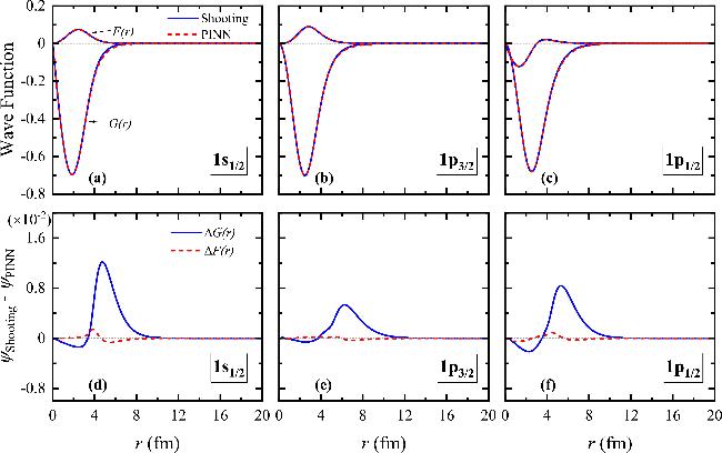
Figure 2. The obtained wave functions of the neutron orbitals 1s1/2 (a), 1p3/2 (b) and 1p1/2 (c) of 16O by the PINN (dashed lines), in comparison with the shooting method (solid lines). (d), (e) and (f) are the corresponding differences of the wave functions between the PINN and the shooting method. |
To have a closer quantitative comparison, table 2 summarizes the differences of the energies and the wave functions between the PINN and the shooting method. It can be seen that the relative errors of energies are of the order of 10-4~10-3 while the absolute deviations for the three orbitals are within 0.065 MeV. For the wave functions, the RMS errors from the results of the shooting method are about 10-3 for G(r) and 10-4 for F(r). As discussed above, the relative deviations of G(r) and F(r) from the true wave functions are of the same order of magnitude. It is noted that the highest accuracy of energy is obtained for the lowest 1s1/2 orbital, whereas the best descriptions for the wave functions G(r) and F(r) are obtained for the 1p3/2 orbital in which the lowest loss is achieved.
Table 2. The results obtained by the PINN for the three neutron orbitals below the Fermi surface of 16O in Dirac WS potential, in comparison with those by the shooting method. The third and fourth columns are the energies (in MeV) obtained by the shooting method and by the PINN respectively. The value ∆E = EShooting - EPINN denotes the energy difference between the two methods and the σE = |∆E/EShooting| denotes the relative deviation. σG and σF are the RMS errors of the wave functions G(r) and F(r) evaluated at 200 mesh points. Bold values indicate the minimum errors among all orbitals. |
| Orbital | κ | EShooting | EPINN | ∆E | σE | σG | σF |
|---|---|---|---|---|---|---|---|
| 1s1/2 | -1 | -43.1891 | -43.1805 | -0.0086 | 1.99 × 10⁻⁴ | 3.48 × 10⁻³ | 3.21 × 10⁻⁴ |
| 1p3/2 | -2 | -24.6645 | -24.6978 | 0.0333 | 1.35 × 10⁻³ | 1.73 × 10⁻³ | 1.24 × 10⁻⁴ |
| 1p1/2 | 1 | -19.0191 | -19.0828 | 0.0637 | 3.35 × 10⁻³ | 2.64 × 10⁻³ | 2.58 × 10⁻⁴ |
4.2. Heavy nucleus 208Pb
In order to further test the performance of PINN, the neutron orbitals in the Dirac WS potential for heavy nucleus 208Pb are calculated. For 208Pb, it has 82 protons and 126 neutrons, and its ground state is also spherical. Below the neutron magic number N = 126, there exist 22 neutron orbitals in total. Unlike the light nucleus 16O, for most κ blocks, more than one orbital needs to be solved, which is realized by the introduction of the third term ${{ \mathcal L }}_{{\rm{orth}}}$ in the loss function (8 ).
Figure 3 shows the loss and the energy varying with the epochs for the three s1/2 orbitals of 208Pb. As seen in figure 3, the loss and energy gradually vary at the beginning and at the 33938th epoch the mean value of the losses satisfies the conditional threshold ε. After further improvement with the learning rate scheduler, the 1s1/2 orbital is obtained and the corresponding wave functions are saved. Then the orthogonality constraint ${{ \mathcal L }}_{{\rm{orth}}}$ is introduced with Gsum and Fsum being the obtained 1s1/2 wave functions. Correspondingly, the loss shows a sudden increase. With the optimization continuing, the PINN is driven to search the next orbital. At the 70592nd epoch, the conditional threshold ε for the excited 2s1/2 orbital is achieved. Later, the Gsum and Fsum take the summation of wave functions of 1s1/2 and 2s1/2 orbitals, and the PINN is driven to search the third orbital. At the 115044th epoch, the conditional threshold ε for the excited 3s1/2 orbital is achieved. In this way, the PINN can find not only the lowest sate but also the excited states with different n in the same κ block.
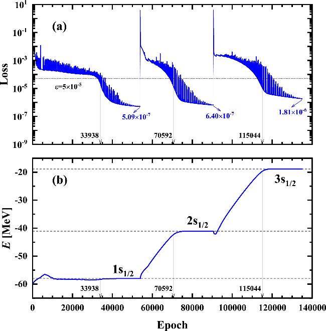
Figure 3. Same as figure 1, but for the neutron orbitals 1s1/2, 2s1/2 and 3s1/2 of 208Pb. |
Figure 4 shows the obtained wave functions for the s1/2 orbitals of 208Pb by the PINN, in comparison with the results by the shooting method. As seen in figures 4(a)-(c), the wave functions obtained by the PINN are in good agreement with those by the shooting method. In figures 4(d)-(f), similar to figure 2, the maximum deviations ∆G(r) and ∆F(r) mainly locate at the tails of the peaks of the wave functions. The absolute differences for the wave functions F(r) are smaller than those of the wave functions G(r), but their relative differences are of the same order of magnitude.
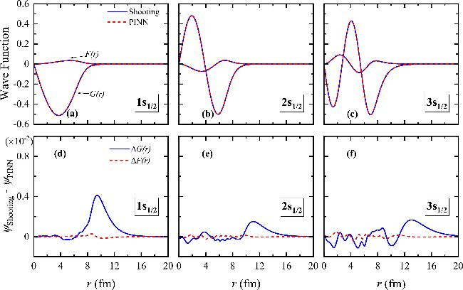
Figure 4. Same as figure 2, but for the neutron orbitals 1s1/2, 2s1/2 and 3s1/2 of 208Pb. |
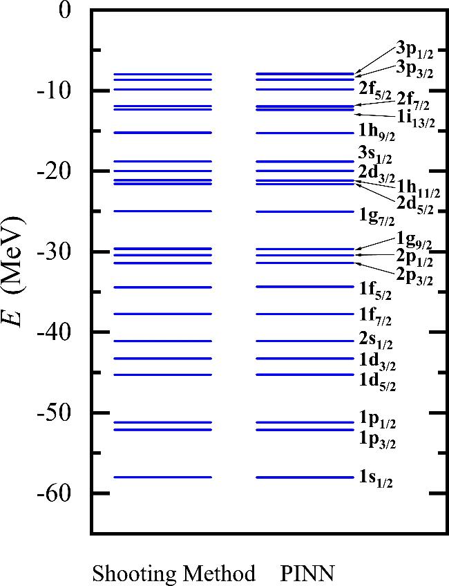
Figure 5 shows the neutron spectrum of 208Pb obtained by the PINN, in comparison with the shooting method. The levels obtained by the PINN show good agreement with those by the shooting method. Table 3 lists the detailed comparisons for all the 22 orbitals below the Fermi surface of 208Pb between the PINN and the shooting method. It can be seen that the relative errors of energies are of the order of 10-3 and the absolute errors are all within 80 keV, showing a satisfying description of PINN to the eigen energies. It is interesting to note that the single-neutron energies obtained by PINN fluctuate above and below those from the shooting method. This indicates that compared to the shooting method, PINN exhibits lower accuracy and larger uncertainties. This characteristic may arise from initialization, random collocation point selection, etc. More importantly, since PINN employs the residual of the Dirac equation as the objective function rather than the variational principle, it allows both overestimation and underestimation of the eigen energies. In contrast, one always yields results not lower than the exact solution if the variational principle for energy expectation values is applied. As for wave functions, the RMS errors of PINN are also of the order of 10-3. The highest energy accuracy is 5.27 × 10⁻⁵ for the 1p1/2 orbital, whereas the best descriptions for the wave functions G(r) and F(r) are obtained 2.72 × 10⁻⁴ for the 1h11/2 orbital and 5.88 × 10⁻⁵ for the 1p3/2 orbital, respectively.
Figure 5. Energy spectrum of neutron for 208Pb in the Dirac WS potential obtained by the PINN, in comparison with the shooting method. |
Table 3. Same as table 2, but for the neutron orbitals below the Fermi surface of 208Pb. |
| Orbital | κ | EShooting | EPINN | ∆E | σE | σG | σF |
|---|---|---|---|---|---|---|---|
| 1s1/2 | -1 | -58.0103 | -58.0272 | 0.0169 | 2.91 × 10⁻⁴ | 1.32 × 10⁻³ | 8.18 × 10⁻⁵ |
| 1p3/2 | -2 | -52.1132 | -52.1209 | 0.0077 | 1.48 × 10⁻⁴ | 8.26 × 10⁻⁴ | 5.88 × 10⁻⁵ |
| 1p1/2 | 1 | -51.1935 | -51.1908 | -0.0027 | 5.27 × 10⁻⁵ | 3.11 × 10⁻³ | 2.30 × 10⁻⁴ |
| 1d5/2 | -3 | -45.2784 | -45.2669 | -0.0115 | 2.54 × 10⁻⁴ | 3.96 × 10⁻³ | 2.67 × 10⁻⁴ |
| 1d3/2 | 2 | -43.2777 | -43.2745 | -0.0032 | 7.39 × 10⁻⁵ | 3.69 × 10⁻³ | 2.65 × 10⁻⁴ |
| 2s1/2 | -1 | -41.1063 | -41.1041 | -0.0022 | 5.35 × 10⁻⁵ | 5.50 × 10⁻⁴ | 7.07 × 10⁻⁵ |
| 1f7/2 | -4 | -37.7301 | -37.7414 | 0.0113 | 2.99 × 10⁻⁴ | 9.00 × 10⁻⁴ | 6.91 × 10⁻⁵ |
| 1f5/2 | 3 | -34.4320 | -34.3547 | -0.0773 | 2.25 × 10⁻³ | 8.13 × 10⁻³ | 6.25 × 10⁻⁴ |
| 2p3/2 | -2 | -31.4324 | -31.4182 | -0.0142 | 4.52 × 10⁻⁴ | 3.82 × 10⁻⁴ | 9.05 × 10⁻⁵ |
| 2p1/2 | 1 | -30.4267 | -30.4508 | 0.0241 | 7.92 × 10⁻⁴ | 1.71 × 10⁻³ | 1.06 × 10⁻⁴ |
| 1g9/2 | -5 | -29.6381 | -29.6543 | 0.0162 | 5.47 × 10⁻⁴ | 7.60 × 10⁻⁴ | 6.49 × 10⁻⁵ |
| 1g7/2 | 4 | -24.9820 | -25.0208 | 0.0388 | 1.55 × 10⁻³ | 5.73 × 10⁻⁴ | 6.35 × 10⁻⁵ |
| 2d5/2 | -3 | -21.5867 | -21.6073 | 0.0206 | 9.54 × 10⁻⁴ | 2.40 × 10⁻³ | 1.38 × 10⁻⁴ |
| 1h11/2 | -6 | -21.1411 | -21.1569 | 0.0158 | 7.47 × 10⁻⁴ | 2.72 × 10⁻⁴ | 8.64 × 10⁻⁵ |
| 2d3/2 | 2 | -19.9730 | -19.9616 | -0.0114 | 5.71 × 10⁻⁴ | 6.98 × 10⁻⁴ | 1.14 × 10⁻⁴ |
| 3s1/2 | -1 | -18.8057 | -18.8206 | 0.0149 | 7.92 × 10⁻⁴ | 7.77 × 10⁻⁴ | 1.40 × 10⁻⁴ |
| 1h9/2 | 5 | -15.2317 | -15.2815 | 0.0498 | 3.27 × 10⁻³ | 3.32 × 10⁻³ | 2.60 × 10⁻⁴ |
| 1i13/2 | -7 | -12.3623 | -12.3852 | 0.0229 | 1.85 × 10⁻³ | 7.64 × 10⁻⁴ | 6.06 × 10⁻⁵ |
| 2f7/2 | -4 | -11.9215 | -11.9617 | 0.0402 | 3.37 × 10⁻³ | 1.77 × 10⁻³ | 1.24 × 10⁻⁴ |
| 2f5/2 | 3 | -9.8662 | -9.8404 | -0.0258 | 2.61 × 10⁻³ | 3.05 × 10⁻³ | 4.10 × 10⁻⁴ |
| 3p3/2 | -2 | -8.6514 | -8.6284 | -0.0230 | 2.66 × 10⁻³ | 5.09 × 10⁻⁴ | 1.26 × 10⁻⁴ |
| 3p1/2 | 1 | -7.9710 | -7.9310 | -0.0400 | 5.02 × 10⁻³ | 2.11 × 10⁻³ | 2.69 × 10⁻⁴ |
Finally, we add a short note on computational cost. When benchmarked on identical CPU hardware and using the present deep NN architecture (Nlay = 3, Nneu = 80), the computation time required by PINN to solve for an orbital is about 107 times longer than that of the shooting method. This is because the PINN has to train a neural network with more than 13000 parameters. One of PINN's key advantages lies in handling high-dimensional complex problems [53], however for the solving of the radial Dirac equation, this advantage has not yet been exploited.
It is also mentioned that some other ML approaches have been employed to solve quantum mechanics problems in nuclear physics. For instance, in [42, 43], the variational Monte Carlo calculations with an artificial neural network (VMC-ANN) achieved a precision better than 0.5 MeV in calculating the ground-state energy of 4He. In [44], The deep-neural-network FeynmanNet reached within 30 keV accuracy for the ground-state energy of 4He. Note that both VMC-ANN and FeynmanNet solve nuclear many-body problems by using the variational principles and serve as ab initio calculations. Here the PINN approach gives an accuracy within 0.1 MeV for solving the single-particle energies. More recently, by using the variational principles, a deep neural network has achieved an accuracy within 10-3 MeV for the single-particle energies [49]. Nevertheless, the PINN approach is not based on the variational principles, and how to improve the accuracy and to address many-body problems in the PINN framework remain problems that warrant further investigation.
5. Summary
In summary, an unsupervised PINN model has been built to solve the nuclear Dirac WS potential, and taking 16O and 208Pb as examples, the energies and wave functions of the neutron orbitals below the Fermi surface have been solved with a satisfactory accuracy. Unlike traditional approaches that rely on the variation of energy expectation value, the PINN directly employs the residual of the Dirac equation as its objective function, thereby avoiding the variational collapse problem naturally. By integrating automatic differentiation techniques, the model overcomes the Fermion doubling problem typically encountered when solving the Dirac equation with the central difference method. An orthogonality constraint has been incorporated into the model to automatically find the excited states. Finally, in comparison with the standard results obtained from the shooting method, the relative errors of the calculated energies and the RMS errors of the wave functions for all three orbitals of 16O and 22 orbitals of 208Pb are on the order of 10-3, demonstrating the satisfactory level of accuracy and reliability of the PINN model.
Although the current testing of the model has shown the feasibility of PINN in solving Dirac equations with potentials that can closely approximate the real nuclear potentials. There are several aspects that demand further exploration and optimization.
First, an important issue lies in further improving the accuracy of PINN. In this paper, the accuracy of PINN is on the order of 10-3 in solving the Dirac equation and stable for both ground states and excited states, which is comparable to the accuracy of the original PINN in solving the nonlinear Schrödinger equation [50]. In recent reviews [52-54], advancements in PINN methodologies to boost efficiency and accuracy have been summarized, including adopting more sophisticated network architectures (e.g., convolutional neural networks/recurrent neural networks) and optimization algorithms (e.g., the L-BFGS-B optimizer), etc. In the next step, incorporating these enhancements is expected to improve the accuracy of PINN in solving the Dirac equation.
Second, the present tests are only on the deeply bound orbitals below the Fermi surface. Further evaluations to the weakly bound orbitals above the Fermi surface for stable nuclei and to the states in exotic nuclei are necessary. It is also interesting to explore the single-particle resonance states above the continuum threshold in the framework of PINN.
Third, the search for excited states may fail sometimes and the computational costs of the PINN is currently expensive. It is worth exploring more robust ways to search for the excited states and reducing the computational costs by refining the optimization process.
Fourth, the currently solved Dirac equation is merely the radial equation, i.e., the spherical symmetry is imposed. Extending the PINN to solve the Dirac equations in three-dimensional coordinates is straightforward and not overly challenging, as NN can simultaneously and efficiently represent the residuals of multiple coupled equations. This extension enables the calculations of more realistic deformed nuclear potentials. Moreover, the PINN can also be applied to solve the time-dependent Dirac equation for dynamical evolution, given its prior success in handling the time-dependent Schrödinger equation [50].
Last but not the least, given that atomic nuclei are self-bound systems, a crucial query is whether PINN can obtain a self-consistent solution of the nuclear density functional. In principle, PINN provides a viable option, but issues regarding self-consistent iteration, solution accuracy and computational efficiency must be resolved. Since self-consistent iterations inherently require substantial computational costs. Therefore, the approach to obtaining self-consistent solutions warrants careful consideration, for instance, exploring whether NN's representational capacity can be leveraged to solve the self-consistent potential field and single-particle wave functions in a synchronized manner.