


1. Introduction
The accelerated expansion of the Universe refers to the phenomenon where the rate at which galaxies move away from each other increases over time. The idea of the Universe's accelerated expansion is vital as it significantly enhances our understanding of the cosmos and its eventual destiny. Observations of distant supernovae [1], cosmic microwave background radiation [2] and the baryonic acoustic oscillations [3] have provided compelling evidence for this behavior. These data indicate that the primary driver of this phase transition is a mysterious force known as dark energy (DE) [4]. It makes up about 68.3% of the total energy in the cosmos, yet its true nature remains unknown. DE's discovery has challenged our understanding of gravity and cosmic evolution, making it one of the most profound mysteries in modern astrophysics. Unveiling its origin could reshape fundamental physics and offer new insights into the Universe's fate. Several DE models and modified gravity theories have been introduced to investigate the impact of DE on the expansion of the Universe [5-8].
Modified theories of gravity extend the framework of general relativity (GR) to address phenomena that GR alone struggles to explain [9-13]. GR, proposed by Einstein, describes gravity as the curvature of spacetime caused by matter and energy. While highly successful in explaining many aspects of cosmic evolution, GR faces challenges in the context of large-scale dynamics and quantum gravity. Modified gravity theories often begin with the Einstein-Hilbert action, which forms the foundation of GR and introduce additional terms or fields to account for observed discrepancies. For instance, f(R) gravity [14] generalizes Einstein's GR by replacing the Ricci scalar R in the Einstein-Hilbert action with a nonlinear function f(R). This modification introduces higher-order curvature corrections that can explain cosmic acceleration without invoking DE. Unlike GR, f(R) theories predict scale-dependent gravitational effects, enabling them to simultaneously address large-scale cosmological phenomena (e.g. late-time expansion) and small-scale solar system tests. However, they face challenges such as instabilities and fine-tuning requirements to match observations. By incorporating additional curvature terms, f(R) gravity provides a geometric alternative to DE, though its viability depends on stringent theoretical and observational constraints.
The matter is essential in shaping the Universe, as its interaction with spacetime generates the gravitational effects seen in everything from planetary motions to the large-scale structure of the cosmos. Curvature-matter coupling [15] has recently gained significant attention as it provides an alternative approach to understanding gravity and the Universe's evolution. This concept involves a direct interaction between the curvature of spacetime, described by geometric quantities like the Ricci scalar, and the matter content of the Universe, represented by the energy-momentum tensor or other matter fields. For instance, in f(R, T) gravity [15], the gravitational action includes functions of both the Ricci scalar (R) and the trace of the energy-momentum tensor (T), allowing matter properties to directly influence the geometry of spacetime. This coupling provides a more flexible framework to model DE, non-conserved matter fields and exotic fluids. However, it introduces energy-momentum non-conservation ($\text { ∇ }$μTμν ≠ 0), requiring careful physical interpretation. Compared to f(R), the f(R, T) gravity can better describe inhomogeneous cosmologies and matter-dominated epochs but demand additional constraints to avoid theoretical inconsistencies.
While f(R) gravity avoids DE by modifying spacetime curvature, it suffers from ghost instabilities and struggles to satisfy both cosmological and local gravity constraints simultaneously. The f(R, T) framework attempts to resolve this by coupling geometry to matter, but at the cost of violating energy-momentum conservation ($\text { ∇ }$μTμν ≠ 0), leading to unphysical scenarios unless ad hoc conditions are imposed. Both theories face difficulties in high-curvature regimes, where singularities and instability risks persist. These shortcomings motivated Amendola et al [16] to introduce Ricci inverse gravity, a modified theory that incorporates the anti-curvature tensor Aαβ, defined by the relation $({A}_{\alpha \beta }{R}^{\beta \sigma }={\delta }_{\alpha }^{\sigma })$, which is closely related to the Ricci tensor, into the gravitational framework. By retaining second-order field equations and avoiding matter-coupling ambiguities, it provides a more stable and geometrically consistent approach to unifying early and late-time cosmic acceleration without relying on unverified matter fields or fine-tuned parameters.
This theory was proposed to explore new avenues for explaining cosmological phenomena, particularly the accelerated expansion of the Universe, without relying on exotic DE components. The key feature of this theory is the introduction of the anti-curvature scalar A = gαβAαβ, which is distinct from the inverse of the Ricci scalar. In a later study, Das et al [17] examined two different types of Ricci-inverse models. Class I model are represented by the f(R, A) gravity while class II model, on the other hand, is given by f(R, AαβAαβ). This formulation provides a broader range of solutions applicable to high-curvature regimes, such as early universe evolution and cosmic singularities, without the instabilities present in previous models. Despite its potential, the role of the anticurvature term in cosmic expansion and thermodynamic stability remains unexplored.
Bouncing cosmology [18] proposes an attractive solution to the initial singularity problem, which is a relatively appealing aspect of cosmological theories. This is due to the fact that in bouncing cosmology, the Universe contracts till it reaches its minimum radius, at which it expands. As a result, the Universe cannot collapse to a singular point, preventing the initial singularity. There are two major categories of cosmological bounces, loop quantum cosmology (LQC) [19] and matter bounce theories [20]. It is interesting to mention here that the scalar fields are used in these types of theories to avoid the singularities and create bounces [18, 20]. Modified gravity also provides a unified explanation of bouncing cosmology [21, 22]. Some drawbacks of bouncing cosmologies include ghost and primordial instabilities during the contracting phase [23], making the contracting phase a hazardous era during evolution. In the framework of Galileon and ghost condensate models, ghost instabilities can be accomplished [24] and the issue related to the contracting phase is fully answered from the perspective of ekpyrotic contraction [25].
Recently, a lot of researchers addressed bouncing cosmologies to show the accelerating expansion of the Universe. The concept of cyclic or ekpyrotic [26, 27] is exhibited through these theories which mean that the Universe is contracting and expanding cyclically. This phenomenon has tested for well-known modified theories like f(G) [28] and f(R) [29] gravity. The ekpyrosis bounce and superbounce are the source of attention and interest [30, 31] with significant contributions provided in [21, 22]. The DE models as well as modified gravity theories are presented in [32, 33] with detail. Some important results of bouncing cosmology are analyzed using f(T, B) gravity. Recently, Jawad and Sultan [34] have worked on different cosmological bouncing scenarios by considering Weyl tensor corrected f(R) gravity.
In this work, we investigate f(R, A) gravity in the context of bouncing cosmologies, which replace the Big Bang singularity with a smooth contraction-to-expansion transition. For this study, we adopt the minimal model f(R, A) = R + αA-1, where α is a dimensionless coupling constant. We analyze five well-studied bouncing modelssymmetric, oscillatory, matter, little rip and superbounce to evaluate the cosmic evolution via the effective equation of state (EoS) parameter (ωeff), identifying phase transitions (quintessence to phantom). We also compute the stability of underlying scenario through the squared speed of sound parameter $({v}_{s}^{2}$). We analyze the thermodynamic consistency by using the generalized second law (GSLT) and thermal equilibrium conditions. It is interesting to mention here that our results demonstrate that f(R, A) gravity provides a stable, thermodynamically viable framework for bouncing universes, with (ωeff) exhibiting realistic phase transitions across all scenarios. Finally, the ${\omega }_{\mathrm{eff}}-{\omega }_{\mathrm{eff}}^{{\prime} }$ plane demonstrates the thawing as well as the freezing region of the universe. This positions f(R, A) as a compelling alternative to conventional modified gravity theories.
This paper is arranged in the following sequence: In upcoming section, we assumed f(R, A) gravity using flat FRW metric and provide basic expressions for this gravity. We also discuss mathematical relations of the effective EoS parameter, squared speed of sound parameter, GSLT and thermal equilibrium condition. In section 3 , we presented a general expression of well-known spectral index and tensor-to-scalar ratio in f(R, A) gravity. In section 4 , some bouncing cosmologies models are assumed and investigate the evolution of universe through some cosmological parameters like EoS ωeff, ${\omega }_{\mathrm{eff}}-{\omega }_{\mathrm{eff}}^{{\prime} }$ plane and stability analysis (squared speed of sound ${v}_{s}^{2}$). We also check the validity of generalized second law of thermodynamics and thermal equilibrium through the expressions of ${T}_{A}{\dot{S}}_{A\mathrm{tot}}$ and ${\ddot{S}}_{A\mathrm{tot}}$ respectively. Finally, we evaluate the In section 5 , we summarize their results.
2. Basic equations of f(R, A) theory, cosmic parameters and thermal implications
In this section, we start with the action of modified Ricci-inverse gravity as [16]
$\begin{eqnarray}S=\int \sqrt{-g}[f(R,A)+{L}_{m}]{{\rm{d}}}^{4}x,\end{eqnarray}$
where g, Lm are the determinant of the metric tensor and matter Lagrangian that is minimally coupled to gravity. The arbitrary function f(R, A) depends upon the Ricci scalar R and anticurvature scalar A, which is the trace of anticurvature tensor Aμν assumed to be the inverse Ricci tensor i.e. ${A}^{\mu \nu }={R}_{\mu \nu }^{-1}$ [16]. It is important to note that A ≠ R-1. Varying the above action with respect to (w.r.t) to the metric tensor gμν, it leads the following field equations of f(R, A) theory as [16] $\begin{eqnarray}\begin{array}{l}{f}_{R}{R}^{\mu \nu }-{f}_{A}{A}^{\mu \nu }-\frac{1}{2}f{g}^{\mu \nu }+{g}^{\rho \mu }{{\rm{\nabla }}}_{\alpha }{{\rm{\nabla }}}_{\rho }{f}_{A}{A}_{\sigma }^{\alpha }{A}^{\nu \sigma }\\ -\frac{1}{2}{{\rm{\nabla }}}^{2}({f}_{A}{A}_{\sigma }^{\mu }{A}^{\nu \sigma })-\frac{1}{2}{g}^{\mu \nu }{{\rm{\nabla }}}_{\alpha }{{\rm{\nabla }}}_{\beta }({f}_{A}{A}_{\sigma }^{\alpha }{A}^{\beta \sigma })\\ -{{\rm{\nabla }}}^{\mu }{{\rm{\nabla }}}^{\nu }{f}_{R}+{g}^{\mu \nu }{{\rm{\nabla }}}^{2}{f}_{R}={T}^{\mu \nu },\end{array}\end{eqnarray}$
where fR and fA are the partial derivatives w.r.t. arguments while $\text { ∇ }$μ represents the covariant derivative. Here energy momentum tensor Tμν is defined as [35] $\begin{eqnarray}{T}^{\mu \nu }=\frac{2}{\sqrt{-g}}\frac{\delta (\sqrt{-g}{L}_{m})}{\delta {g}_{\mu \nu }}.\end{eqnarray}$
Next, we consider the flat FRW metric with scale factor a(t) and energy momentum tensor for perfect fluid content. For this metric, we get the anticurvature scalar A [16] as $A=\frac{2(6+5\epsilon )}{3{H}^{2}(1+\epsilon )(3+\epsilon )}$, where $\epsilon =\frac{H^{\prime} }{H}$ and $H=\frac{\dot{a}}{a}$, the prime and dot represent the derivative w.r.t. ${\mathrm{ln}}\,a$ and time t respectively. The f(R, A) gravity simply depends on the selection of f(R, A) model. In this context, a lot of models have been proposed, we pick the following simplest model for f(R, A) gravity as [16] $\begin{eqnarray}f(R,A)=R+\alpha {A}^{-1},\end{eqnarray}$
where α is a dimensionless constant. The parameter α in f(R, A) gravity plays a crucial role in determining the contribution of the anticurvature term A in the modified field equations. It acts as a coupling constant that controls the relative strength of the anticurvature effects compared to the Ricci scalar R. The natural scale of α depends on the underlying theoretical framework, and its value can, in principle, be constrained by observational data (Planck 2018) related to cosmic expansion, structure formation, and thermodynamic behavior. For instance, cosmological observations such as supernovae data, cosmic microwave background fluctuations, and baryon acoustic oscillations can provide bounds on α by comparing theoretical predictions with empirical results. The sign of α significantly influences cosmic dynamics-positive values tend to enhance repulsive effects, potentially leading to accelerated expansion, while negative values may introduce modifications that influence early universe behavior and bouncing scenarios.For underlying model, the corresponding field equations are reduced to the form
$\begin{eqnarray}3{H}^{2}={k}^{2}{\rho }_{\mathrm{eff}},\quad -(2\dot{H}+3{H}^{2})={k}^{2}{P}_{\mathrm{eff}},\end{eqnarray}$
where $\begin{eqnarray}{\rho }_{\mathrm{eff}}=\rho -3\alpha {H}^{2}\displaystyle \frac{{(\epsilon +3)}^{2}(5\epsilon +6)-18\epsilon ^{\prime} }{4{(5\epsilon +6)}^{3}},\end{eqnarray}$
$\begin{eqnarray}\begin{array}{rcl}{P}_{\mathrm{eff}} & = & P+2{H}^{2}\epsilon -2\dot{H}+\displaystyle \frac{\alpha {H}^{2}}{4{(5\epsilon +6)}^{4}}\Space{0ex}{2.5ex}{0ex}[(5\epsilon +6)\\ & & \times \left\{\Space{0ex}{2.15ex}{0ex}{(\epsilon +3)}^{2}(2\epsilon +3)(5\epsilon +6)-18\epsilon ^{\prime\prime} \Space{0ex}{2.15ex}{0ex}\right\}\\ & & +270{({\epsilon }^{^{\prime} })}^{2}-54(\epsilon +2)(5\epsilon +6){\epsilon }^{{\prime} }\Space{0ex}{3.10ex}{0ex}].\end{array}\end{eqnarray}$
In this scenario, the conservation law leads to the following continuity equation as $\begin{eqnarray}{\dot{\rho }}_{\mathrm{eff}}+3H({\rho }_{\mathrm{eff}}+{P}_{\mathrm{eff}})=0.\end{eqnarray}$
Next, we investigate the cosmic aspects of f(R, A) theory of gravity through the cosmological parameters like EoS parameter and squared speed of sound parameter. These parameters play a vital role in evaluating different characteristics of the Universe. We also discuss the thermodynamical aspects of f(R, A) gravity through GSLT. We also check the thermal equilibrium condition through second derivative of the total entropy.2.1. Equation of state parameter
The EoS parameter (ω) is a basic tool to examine the evolution of the Universe and have mathematical expression as ${\omega }_{\mathrm{eff}}=\tfrac{{P}_{\mathrm{eff}}}{{\rho }_{\mathrm{eff}}}$. One can explore the decelerated as well as accelerated phases of universe through this parameter. The decelerated phases of universe is defined as follow 2.7 ) by equation (2.6 ), we get an expression the EoS parameter as
$\begin{eqnarray}{\omega }_{\mathrm{Dec}}=\left\{\begin{array}{cc}\mathrm{Stiff}\,\mathrm{fluid} & \mathrm{if}\,\omega =1,\\ \mathrm{Radiation}\rm{-}\mathrm{dominated}\,\mathrm{era} & \mathrm{if}\,\omega =\displaystyle \frac{1}{3},\\ \mathrm{Matter}\rm{-}\mathrm{dominated}\,\mathrm{era} & \mathrm{if}\,\omega =0.\end{array}\right.\end{eqnarray}$
The accelerated phases of universe is given as $\begin{eqnarray}{\omega }_{\mathrm{Acc}}=\left\{\begin{array}{cc}\mathrm{Quintessence} & \mathrm{if}\,-1\lt \omega \lt -\displaystyle \frac{1}{3},\\ \mathrm{Cosmological}\,\mathrm{constant} & \mathrm{if}\,\omega =-1,\\ \mathrm{Phantom}\rm{-}\mathrm{dominated}\,\mathrm{era} & \mathrm{if}\,\omega \lt -1.\end{array}\right.\end{eqnarray}$
Dividing equation ( $\begin{eqnarray}\begin{array}{l}{\omega }_{\mathrm{eff}}=-\displaystyle \frac{\alpha }{(6{H}^{2}+5\dot{H})}\Space{0ex}{2.5ex}{0ex}[(3{H}^{2}(5{\dot{H}}^{3}+72{H}^{2}{\dot{H}}^{2}+81{H}^{4}\dot{H}\\ \,+\,54{H}^{6}-18{H}^{3}\ddot{H})\alpha -4(6{H}^{2}+5\dot{H}){\rho }_{m}{)}^{-1}\{-270{H}^{4}\\ \,\times \,{\ddot{H}}^{2}+540{H}^{10}+828{H}^{8}\dot{H}-50{\dot{H}}^{5}-1940{H}^{2}{\dot{H}}^{4}\\ \,-\,1646{H}^{4}{\dot{H}}^{3}+18{\ddot{H}}^{2}(18{H}^{7}+26{H}^{5}\dot{H})+75{H}^{3}{\dot{H}}^{2}\\ \,+\,{H}^{6}(-681{\dot{H}}^{2}+18\dddot{H})\Space{0ex}{3.10ex}{0ex}].\end{array}\end{eqnarray}$
2.2. Squared speed of sound parameter
The squared speed of sound parameter ${v}_{s}^{2}=\tfrac{{\rm{d}}{P}_{\mathrm{eff}}}{{\rm{d}}{\rho }_{\mathrm{eff}}}$ is a crucial factor in determining the stability of cosmological models within perturbation theory and gravitational wave analysis. For a model to be stable, ${v}_{s}^{2}$ must be non-negative, ensuring that small perturbations propagate without unbounded growth. When ${v}_{s}^{2}\gt 0$, perturbations travel as waves, preventing any exponential divergence. However, if ${v}_{s}^{2}\lt 0$, the system becomes unstable due to the rapid growth of perturbations, making the model physically inconsistent. In the study of gravitational waves, stability is achieved when the kinetic term of tensor perturbations remains positive, preventing the occurrence of ghost instabilities. In modified gravity frameworks like f(R, A) gravity, additional geometric contributions can influence the behavior of perturbations. Therefore, it is essential to confirm that these modifications do not introduce instability or superluminal propagation. A stable model must ensure ${v}_{s}^{2}\geqslant 0$ at all times while also maintaining a gravitational wave speed within observational limits set by detectors such as LIGO and Virgo. If these criteria are met, the model can be considered viable without suffering from perturbative instabilities. Differentiating equations (2.7 ) and (2.6 ) w.r.t. t and then dividing the resulting equations, we obtain ${v}_{s}^{2}$ for modified f(R, A) gravity in appendix 6.1.
2.3. Thermodynamical analysis
Thermodynamical analysis in cosmology involves applying the principles of thermodynamics to the large-scale structure and evolution of the Universe. Central to this analysis is the study of entropy, temperature and energy exchanges at different cosmic scales, such as the cosmic horizon, black holes, and the expanding universe. In the cosmological context, the GSLT plays a crucial role, extending the traditional Second Law to account for systems with horizons, like the Universe itself or black holes. According to GSLT, the total entropy, which includes both the matter and horizon entropy contributions, should not decrease over time $({\dot{S}}_{\mathrm{int}}+{\dot{S}}_{\mathrm{ext}}\gt 0)$. This law is particularly significant in models of cosmic evolution, where horizon entropy changes due to the expansion of the Universe, the presence of DE, and the dynamics of spacetime curvature. This thermodynamical perspective provides valuable insights into the stability, evolution, and ultimate fate of the Universe within different cosmological frameworks.
Black holes offer a critical framework for establishing a connection between gravitational physics and thermodynamics [36]. Further investigations by Bekenstein and Hawking [37, 38] highlighted the significant role quantum physics plays in understanding the thermodynamic properties of black holes. In 1973, Bekenstein [37, 39] proposed that the entropy of a black hole, treated as a thermodynamic quantity, is directly related to the area of its event horizon, which is a geometrical entity. This conjecture was later validated by Hawking, who introduced the Bekenstein-Hawking (BH) formula $S=\frac{A}{4}$, where S represents entropy and A is the horizon area. Additionally, Hawking demonstrated that black holes emit thermal radiation due to quantum effects [38-40]. These quantum effects enable a physical interpretation of the laws of black hole mechanics, aligning them with the standard laws of thermodynamics [41-44]. Furthermore, Jacobson [45] used Q (heat), S (entropy) and ${ \mathcal T }$ (temperature) and proposed a fundamental relation named Clausius relation and is defined as $\delta Q={ \mathcal T }\delta S$ with the proportionality of horizon area to entropy. For FRW universe, Cai and Kim [46] considered Hawking temperature $({{ \mathcal T }}_{A}=\frac{1}{2\pi {R}_{A}})$ and Bekenstein entropy $({S}_{A}=\frac{\pi {R}_{A}^{2}}{G})$ with the apparent horizon $({R}_{A}=\frac{1}{H})$ and constructed the Friedmann equation in terms of the first law of thermodynamics. The law of thermodynamics is defined as 2.12 ) and taking time derivative gives 2.6 ), we get the value of ${\dot{\rho }}_{\mathrm{eff}}$ as 2.6 ), (2.7 ) and (2.14 ) in equation (2.13 ), we acquire the internal entropy in appendix 6.2. Wald [47] proposed horizon entropy with neother charge that is in general different from Bekenstein entropy. The Wald's entropy in f(R, A) gravity leads to 2.4 ) in equation (2.15 ), yields the following relation 2.16 ) takes the following form 2.17 ) with Hawking temperature that is given $T=\frac{H}{2\pi }$, we get A2 ) and (2.18 ) in appendix 6.3.
$\begin{eqnarray}{T}_{A}{\rm{d}}{S}_{IA}=P{\rm{d}}{V}_{A}+{\rm{d}}{E}_{IA},\end{eqnarray}$
where SIA is the internal entropy of system while ${V}_{A}=\frac{4\pi }{3{H}^{3}}$ and EIA = ρVA. Inserting these values in ( $\begin{eqnarray}{T}_{A}{\dot{S}}_{IA}=\displaystyle \frac{4\pi }{{H}^{3}}\left[\displaystyle \frac{\dot{{\rho }_{\mathrm{eff}}}}{3}-({\rho }_{\mathrm{eff}}+{P}_{\mathrm{eff}})\displaystyle \frac{\dot{H}}{H}\right].\end{eqnarray}$
Differentiate equation ( $\begin{eqnarray}\begin{array}{rcl}{\dot{\rho }}_{\mathrm{eff}} & = & {\dot{\rho }}_{m}-\displaystyle \frac{3\alpha H}{2{(6{H}^{2}+5\dot{H})}^{4}}\Space{0ex}{2.5ex}{0ex}[9{\ddot{H}}^{2}(15{H}^{4}+24{H}^{3}{\dot{H}}^{2}\\ & & +20H{\dot{H}}^{3})+\dot{H}(324{H}^{8}+1080{H}^{6}\dot{H}+999{H}^{4}{\dot{H}}^{2}\\ & & +840{H}^{2}{\dot{H}}^{3}+25{\dot{H}}^{4}+216{H}^{3}{\dot{H}}^{2}\dddot{H}+180H{\dot{H}}^{3}\dddot{H})\\ & & -9\ddot{H}\{18{H}^{7}+21{H}^{5}\dot{H}+65{H}^{3}{\dot{H}}^{2}+20{\dot{H}}^{5}+24{H}^{4}\\ & & \times \dot{H}\dddot{H}+4{H}^{2}(6{\dot{H}}^{4}+5{\dot{H}}^{2}\dddot{H})\}\Space{0ex}{2.95ex}{0ex}].\end{array}\end{eqnarray}$
Putting equations ( $\begin{eqnarray}{S}_{A}=\frac{A}{4G}{f}_{R}.\end{eqnarray}$
Substituting equation ( $\begin{eqnarray}{S}_{A}=\frac{\pi }{G}\left[\frac{1}{{H}^{2}}\right],\end{eqnarray}$
the times derivative of equation ( $\begin{eqnarray}{\dot{S}}_{A}=-\frac{2\pi }{G}\left[\frac{\dot{H}}{{H}^{3}}\right].\end{eqnarray}$
Multiplying on both sides of equation ( $\begin{eqnarray}{T}_{A}{\dot{S}}_{A}=-\frac{1}{G}\left[\frac{\dot{H}}{{H}^{2}}\right].\end{eqnarray}$
Finally, the total entropy ${T}_{A}{\dot{S}}_{A\mathrm{tot}}={T}_{A}{\dot{S}}_{A}+{T}_{A}{\dot{S}}_{IA}$ is obtained by using equations (2.4. Thermal equilibrium
This condition ensures the thermal stability of a system, indicating that the total entropy has reached a local maximum, i.e. $({\ddot{S}}_{A\mathrm{tot}}\lt 0)$ [48]. In thermodynamics, equilibrium is attained when entropy is maximized, and this criterion confirms that any small perturbation will not spontaneously increase the entropy further . If ${\ddot{S}}_{A\mathrm{tot}}\gt 0$, the system is unstable, as entropy can still increase. This principle is crucial in analyzing the second law of thermodynamics and stability in cosmological and gravitational thermodynamic frameworks.
Now, we check the thermal condition of underlying model, for this first we write the simplified form of equation (A3 ) as 2.19 ) w.r.t. t, it yields the expression ${\ddot{S}}_{A\mathrm{tot}}$ in appendix 6.4.
$\begin{eqnarray}\begin{array}{rcl}{\dot{S}}_{A\mathrm{tot}} & = & -\displaystyle \frac{2\pi }{G}\left[\displaystyle \frac{\dot{H}}{{H}^{3}}\right]+\displaystyle \frac{8{\pi }^{2}}{{H}^{4}}\left[\displaystyle \frac{{\dot{\rho }}_{m}}{3}-\displaystyle \frac{\alpha H}{2{(6{H}^{2}+5\dot{H})}^{4}}\right.\\ & & \times \Space{0ex}{3.25ex}{0ex}\{9{\ddot{H}}^{2}(15{H}^{4}+24{H}^{3}{\dot{H}}^{2}+20H{\dot{H}}^{3})+\dot{H}(324{H}^{8}\\ & & +1080{H}^{6}\dot{H}+999{H}^{4}{\dot{H}}^{2}+840{H}^{2}{\dot{H}}^{3}+25{\dot{H}}^{4}\\ & & +216{H}^{3}{\dot{H}}^{2}\dddot{H}+180H{\dot{H}}^{3}\dddot{H})-9\ddot{H}(18{H}^{7}+21\\ & & \times {H}^{5}\dot{H}+65{H}^{3}{\dot{H}}^{2}+20{\dot{H}}^{5}+24{H}^{4}\dot{H}\dddot{H}+4{H}^{2}\\ & & \times (6{\dot{H}}^{4}+5{\dot{H}}^{2}\dddot{H}))\Space{0ex}{3.10ex}{0ex}\}-\left[{\rho }_{m}+\displaystyle \frac{1}{4{(6{H}^{2}+5\dot{H})}^{4}}\right.\\ & & \times \Space{0ex}{3.40ex}{0ex}\{270{H}^{4}{\ddot{H}}^{2}-540{H}^{10}-828{H}^{8}\dot{H}+1646{H}^{4}{\dot{H}}^{3}\\ & & +1940{H}^{2}{\dot{H}}^{4}+50{\dot{H}}^{5}-18\ddot{H}(18{H}^{7}+26{H}^{5}\dot{H}\\ & & +\left.\left.75{H}^{3}{\dot{H}}^{2})+3{H}^{6}(227{\dot{H}}^{2}-6\dddot{H})\Space{0ex}{3.40ex}{0ex}\}\alpha \Space{0ex}{3.40ex}{0ex}\right]\displaystyle \frac{\dot{H}}{H}\right].\end{array}\end{eqnarray}$
Next, we differentiate equation (2.5. ${\omega }_{\mathrm{eff}}-{\omega }_{\mathrm{eff}}^{{\prime} }$ plane
The ${\omega }_{\mathrm{eff}}-{\omega }_{\mathrm{eff}}^{{\prime} }$ plane, is a diagnostic tool used to classify the evolution of DE models. It originates from the EoS parameter ωeff and its derivative ${\omega }_{\mathrm{eff}}^{{\prime} }=\tfrac{{\rm{d}}{\omega }_{\mathrm{eff}}}{\mathrm{dln}a(t)}$ [49]. This plane is particularly useful for distinguishing between 'thawing' and 'freezing' scalar field models of DE. Thawing models begin with ωeff < 0 and evolve towards less negative values with ${\omega }_{\mathrm{eff}}^{{\prime} }\gt 0$, while freezing models start with ωeff < 0 and slow down over time, leading to ${\omega }_{\mathrm{eff}}^{{\prime} }\lt 0$. Different regions of this plane help in understanding the nature of cosmic acceleration and setting observational targets for future cosmological studies. One can obtain the expression of ${\omega }_{\mathrm{eff}}^{{\prime} }$ by differentiating ωeff with respect to ${\mathrm{ln}}\,a$.
3. A general expression of tensor-to-scalar ratio in f(R, A) bouncing cosmology
The evolution of the Universe within a general bouncing cosmology is characterized by two primary phases: a contraction phase followed by an expansion phase. Some of the widely recognized scale factors associated with a non-singular bounce are given by $a(t)={{\rm{e}}}^{\alpha {t}^{2}}$, $a(t)=\cosh t$, $a(t)\,={({a}_{0}{t}^{2}+1)}^{n}$, $a(t)={{\rm{e}}}^{\tfrac{1}{\alpha +1}{(t-\beta )}^{\alpha +1}}$. These forms represent various mathematical models for describing non-singular bouncing scenarios in cosmology. At the bouncing point, the Hubble parameter becomes zero and consequently, the comoving Hubble radius, defined as ${r}_{h}=\frac{1}{aH}$, diverges. This behavior is consistent across all the aforementioned models. However, the asymptotic behavior of the comoving Hubble radius varies among these bouncing models. Specifically, for certain scale factors such as $a(t)={{\rm{e}}}^{\alpha {t}^{2}}$, $a(t)=\cosh t$, and $a(t)={({a}_{0}{t}^{2}+1)}^{n}$ where $n\gt \frac{1}{2}$, the Hubble radius decreases monotonically on either side of the bounce and eventually shrinks to zero asymptotically. This indicates an accelerating universe at late times.
In such cases, the Hubble horizon approaches zero as the cosmic time increases significantly, while near the bouncing point, the Hubble horizon attains an infinite size. Consequently, primordial perturbation modes pertinent to the present era are generated during the period close to the bouncing point, as this is the only interval when all primordial modes are contained within the horizon. As the horizon contracts, these modes exit and become relevant for contemporary observations. In these scenarios, the perturbation modes are generated during very large negative cosmic times, corresponding to the low-curvature regime of the contracting phase, unlike the previous situation where modes are generated near the bouncing point. Specifically, in such cases, the comoving wave number k begins propagating through spacetime during the contracting phase at sub-Hubble scales, exits the Hubble radius in this phase, and re-enters the Hubble radius during the low-curvature regime of the expansion phase at time th(k). Notably, the exit and entry times are symmetric about the bouncing point, as the scale factor exhibits symmetry. This symmetry makes the perturbation modes relevant for present-day observations.
Thus, the physical picture differs significantly between these two cases regarding the generation of perturbation modes. In both scenarios, however, the comoving curvature perturbation must evolve through the contracting phase, the bouncing phase, and into the expanding phase to derive the power spectrum at later times. In the large-scale limit (i.e. the super-Hubble scale k « aH) of the contracting phase, the comoving curvature perturbation ${ \mathcal R }(k,\eta )$ satisfies the cosmological perturbation equation 3.1 ) is expressed as
$\begin{eqnarray}v^{\prime\prime} (k,\eta )-\frac{z^{\prime\prime} (\eta )}{z(\eta )}v(k,\eta )=0,\end{eqnarray}$
where η is the conformal time, v(k, η) is the canonical variable, and z(η) depends on the specific cosmological model. Since, the focus in the current context is on the f(R, A) model, the variable z(η) takes the following form $\begin{eqnarray}z(\eta (t))=\displaystyle \frac{a(t)}{\kappa (H(t)+\tfrac{F^{\prime\prime} (R,A)}{2{F}^{^{\prime} }(R,A)}\tfrac{{\rm{d}}R}{{\rm{d}}t})}\sqrt{\displaystyle \frac{3F^{\prime\prime} (R,A)}{2{F}^{^{\prime} }(R,A)}{\left(\displaystyle \frac{{\rm{d}}R}{{\rm{d}}t}\right)}^{2}}.\end{eqnarray}$
For a general z(η), the solution to equation ( $\begin{eqnarray}{v}_{c}(k,\eta )=z(\eta )\left[{D}_{c}(k)+{S}_{c}(k)\int \displaystyle \frac{{\rm{d}}\eta }{{z}^{2}(\eta )}\right].\end{eqnarray}$
Both Dc(k) and Sc(k) are time-independent and encapsulate information about the spectra of the two modes.The solution for above directly yields the curvature perturbation on the super-Hubble scale during the contracting phase as
$\begin{eqnarray}{{ \mathcal R }}_{c}(k,\eta )=\displaystyle \frac{{v}_{c}(k,\eta )}{z(\eta )}={D}_{c}(k)+{S}_{c}(k)\int \displaystyle \frac{{\rm{d}}\eta }{{z}^{2}(\eta )}.\end{eqnarray}$
As can be seen from the above expression, the D mode is constant, while the S mode typically behaves as an increasing mode. Likewise, in the large-scale limit of the expanding phase, the curvature perturbation takes the following form $\begin{eqnarray}{{ \mathcal R }}_{e}(k,\eta )={D}_{e}(k)+{S}_{e}(k)\int \displaystyle \frac{{\rm{d}}\eta }{{z}^{2}(\eta )}.\end{eqnarray}$
The De mode of the curvature perturbation remains constant over time, similar to the Dc mode in the contracting phase. However, the behavior of the S mode differs significantly. In the expanding phase, Se is the sub-dominant decreasing mode, while in the contracting phase, the situation is reversed, with Sc being the decreasing mode. Consequently, during the expansion period, the dominant mode of curvature perturbations is De. This results in the following power spectrum for the curvature perturbations at late time $\begin{eqnarray}{P}_{e}(k)=\frac{{k}^{3}}{2{\pi }^{2}}| {D}_{e}(k){| }^{2}.\end{eqnarray}$
Likewise, the power spectrum for the tensor perturbation is expressed as ${P}_{e}^{(T)}(k)=\frac{{k}^{3}}{2{\pi }^{2}}| {D}_{e}^{(T)}(k){| }^{2}$. Furthermore, the curvature perturbation must remain continuous, meaning that ${{ \mathcal R }}_{c}$ and ${{ \mathcal R }}_{e}$ need to be matched at the bouncing point, as explicitly demonstrated in [50, 51]. During this matching process, the De mode may acquire contributions from both the Dc and Sc modes [50, 51]. It is worth mentioning that a model is considered viable if observable quantities, such as the spectral index ns and the tensor-to-scalar ratio r defined by ${n}_{s}-1=\tfrac{\mathrm{dln}{P}_{e}}{\mathrm{dln}k}$ and $r=\frac{{P}_{e}(k)}{{P}_{T}(k)}$, are in agreement with the latest observations. Further detailed about this phenomenon has been given in the literature [52].4. Cosmic and thermodynamic aspects
One can avoid the early big bang singularities through bouncing solutions, therefore these bouncing cosmologies play a vital role in modern physics. The basic ideas behind these theories are the results of the application of loop quantum gravity to cosmology. These theories favored a cyclic expansion of the Universe and predict a periodic succession of big crunch and big bang phases. In this section, we will discuss the cosmic and the thermodynamical nature of universe through EoS parameter, ${\omega }_{\mathrm{eff}}-{\omega }_{\mathrm{eff}}^{{\prime} }$ plane and GSLT for appropriate bouncing scale factors. Furthermore, we check the thermal equilibrium condition for all cases and analyze the graphical results using different cosmological models.
4.1. Symmetric bounce
Cai et al [53] introduced this type of cosmology to generate non-singular bouncing. various cosmologists considered this form of cosmology for different nobel modified theories of gravity and found interesting results [54, 55]. We work on the reconstruction of this cosmology and use the following scale factor
$\begin{eqnarray}a(t)=B\exp \left(\frac{\beta {t}^{2}}{{t}_{p}^{2}}\right),\end{eqnarray}$
where B, β > 0 are the real numbers while tp denotes the arbitrary time. One can easily find the expression of Hubble parameter and its higher derivative for this scale factor as $\begin{eqnarray}H(t)=\frac{2\beta t}{{t}_{p}^{2}}.\end{eqnarray}$
$\begin{eqnarray}\displaystyle \frac{{\rm{d}}H}{{\rm{d}}t}=\displaystyle \frac{2\beta }{{t}_{p}^{2}},\quad \displaystyle \frac{{{\rm{d}}}^{2}H}{{\rm{d}}{t}^{2}}=0,\quad \displaystyle \frac{{\rm{d}}{t}^{3}}{{\rm{d}}{a}^{3}}=0,\quad \displaystyle \frac{{\rm{d}}{t}^{4}}{{\rm{d}}{a}^{4}}=0.\end{eqnarray}$
Using this expression of Hubble parameter and its derivatives in equation (2.11 ), we obtain the expression of ωeff. We plot the graph of effective EoS parameter against t as shown in figure 1(i) by taking α = -10, β = 0.2, ts = 1 and different values of B as mentioned in the panel. The plot shows the evolution from the quintessence era to the phantom era traversing the cosmological constant line by increasing the cosmic time t. The squared speed of sound is evaluated in figure 1(ii) using mathematical relation (equation (A1 )) assuming the same constant parameters as in above figure. The graph describes the stable behavior of the underlying model on the interval 2 ≤ t ≤ 3. The GSLT model, that has mathematical expression in equation (A3 ) with Bekenstein entropy assuming apparent horizon as seen in figure 1(iii). It is observed from figure that GSLT is valid for this model. In figure 1(iv), the thermal equilibrium condition is checked mathematically represented in equation (A4 ) that leads to the system being in thermal equilibrium. Similarly, ${\omega }_{\mathrm{eff}}-{\omega }_{\mathrm{eff}}^{{\prime} }$ plane in figure 1(v), is represented to analyze the evolution of DE models. The curves show different trajectories, likely corresponding to various parameter choices or cosmological scenarios. From the plot, we observe that ${\omega }_{\mathrm{eff}}^{{\prime} }\gt 0$ for ωeff < 0 which corresponds to thawing region of the universe.
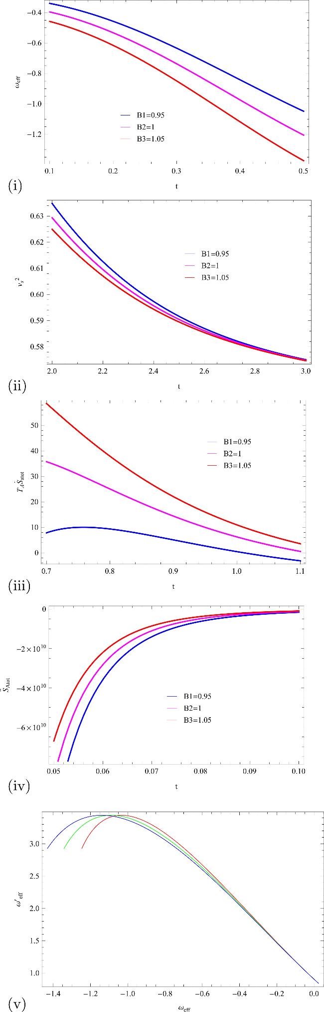
Figure 1. Plots of (i) The plot shows the evolution of the EoS parameter, initially depicting the quintessence era, then transitioning to a cosmological constant phase and finally entering the phantom era. (ii) Squared speed of parameter as the function of t which lead to stability of the underlying model (iii) GSLT $({\dot{S}}_{\mathrm{tot}})$ versus t which corresponds to validity of GSLT (iv) Thermal equilibrium which ensures the thermal stability of a system (v) The ${\omega }_{\mathrm{eff}}-{\omega }_{\mathrm{eff}}^{{\prime} }$ plane demonstrates the thawing region. These plots are drawn for symmetric bounce cosmology. |
4.2. Oscillatory cosmology
This model describes the cyclic behavior of universe [18] which portrays the cosmos as a continuous loop of expansion and contraction [56, 57]. This model having oscillatory scale factor as given following
$\begin{eqnarray}a(t)=B{\sin }^{2}\left(\frac{Ct}{{t}_{s}}\right),\end{eqnarray}$
where B, C > 0 while ts denotes the non-negative reference time. When we choose this scale factor then further two kinds of bouncing behavior arise. The first singularity occurs when $t=\frac{n\pi {t}_{s}}{C}$ (for n ∈ Z) resemble to big bang theory [56]. The second kind is observed when $t=\frac{(2n+1)\pi {t}_{s}}{2C}$, at this stage the Universe reaches its maximum size. For this time, the transition of cosmos changes from expansion to contraction [37]. For this scale factor, Hubble parameter takes the following form $\begin{eqnarray}H(t)=\frac{2C}{{t}_{s}}\cot \left(\frac{Ct}{{t}_{s}}\right).\end{eqnarray}$
One can find the higher derivatives of Hubble parameter as follow $\begin{eqnarray*}\begin{array}{rcl}\dot{H} & = & -\frac{2{C}^{2}{\csc }^{2}\left(\frac{Ct}{{t}_{s}}\right)}{{t}_{s}^{2}},\\ \ddot{H} & = & \frac{4{C}^{3}\cot \left(\frac{Ct}{{t}_{s}}\right){\csc }^{2}\left(\frac{Ct}{{t}_{s}}\right)}{{t}_{s}^{3}},\\ \dddot{H} & = & -\frac{4{C}^{4}{\csc }^{4}\left(\frac{Ct}{{t}_{s}}\right)}{{t}_{s}^{4}}-\frac{8{C}^{4}{\cot }^{4}\left(\frac{Ct}{{t}_{s}}\right){\csc }^{4}\left(\frac{Ct}{{t}_{s}}\right)}{{t}_{s}^{4}},\\ \ddddot{H} & = & \frac{16{C}^{5}{\cot }^{3}\left(\frac{Ct}{{t}_{s}}\right){\csc }^{2}\left(\frac{Ct}{{t}_{s}}\right)}{{t}_{s}^{5}}+\frac{32{C}^{5}\cot \left(\frac{Ct}{{t}_{s}}\right){\csc }^{4}\left(\frac{Ct}{{t}_{s}}\right)}{{t}_{s}^{5}}.\end{array}\end{eqnarray*}$
For oscillatory scale factor, the ωeff which has mathematical relation presented in equation (2.11 ) versus t by assuming C = 0.5, ts = 1.01, B = 1.35 is plotted in figure 2(i). The trajectories of plot lead to the quintessence phase as well as vacuum phase of universe for selected value of t. The plot ${v}_{s}^{2}$ is given in figure 2(ii) using mathematical relation (equation (A1 )) describing the stabile behavior of oscillatory bouncing cosmology. The plot of ${\dot{S}}_{A\mathrm{tot}}$ for apparent horizon by considering Bekenstein entropy as external entropy is indicated in figure 2(iii) using mathematical equation (A3 ) resulting in the satisfaction of GSLT. From mathematical expression (A4 ), we acquire thermal equilibrium term as presented in figure 2(iv). It is found that the system is in equilibrium. The ${\omega }_{\mathrm{eff}}-{\omega }_{\mathrm{eff}}^{{\prime} }$ plot in figure 2(v) shows a parabolic-like trajectory, where ${\omega }_{\mathrm{eff}}^{{\prime} }$ attains significantly negative values for both large positive and negative ωeff. This indicates a rapid variation in the EoS parameter in these regions. However, for ωeff < 0, the curve trends downward, implying that ${\omega }_{\mathrm{eff}}^{{\prime} }\lt 0$ which is a characteristic feature of the freezing region.
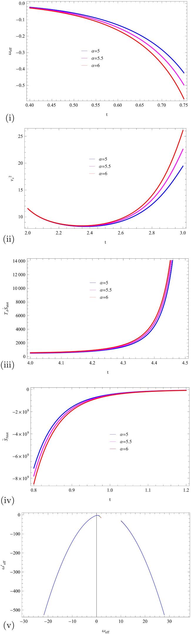
Figure 2. Plots of (i) The plot illustrates the evolution of the EoS parameter, initially depicting the quintessence era, then transitioning to a cosmological constant phase and finally entering the phantom era. (ii) Squared speed of parameter as the function of t which lead to stability of the underlying model (iii) GSLT $({\dot{S}}_{\mathrm{tot}})$ versus t which corresponds to validity of GSLT $({\dot{S}}_{\mathrm{tot}}\gt 0)$ (iv) Thermal equilibrium which ensures the thermal stability of a system $({\ddot{S}}_{\mathrm{tot}}\lt 0)$ (v) The ${\omega }_{\mathrm{eff}}-{\omega }_{\mathrm{eff}}^{{\prime} }$ plane exhibits the freezing region. These plots are drawn for oscillatory bounce cosmology. |
4.3. Matter bounce cosmology
Matter bounce cosmology model is derived from LQC [58, 59]. This model is studied during the early stage evolution of the Universe, the scale factor of matter bounce is defined as
$\begin{eqnarray}a(t)=B{\left(\frac{3}{2}{\rho }_{0}{t}^{2}+1\right)}^{\frac{1}{3}},\end{eqnarray}$
where B ∈ R+ and ρ0 denotes the critical density (derived from LQC) such that 0 < ρ0 « 1. The expression of H for matter bounce cosmology is given by $\begin{eqnarray}H(t)=\frac{2{\rho }_{0}t}{3{\rho }_{0}{t}^{2}+2}.\end{eqnarray}$
Also $\begin{eqnarray}\begin{array}{rcl}\dot{H} & = & \frac{2{\rho }_{0}}{3{\rho }_{0}{t}^{2}+2}-\frac{12{\rho }_{0}^{2}{t}^{2}}{{(3{\rho }_{0}{t}^{2}+2)}^{2}},\\ \ddot{H} & = & \frac{144{\rho }_{0}^{3}{t}^{3}}{{(3{\rho }_{0}{t}^{2}+2)}^{3}}-\frac{36{\rho }_{0}^{2}t}{{(3{\rho }_{0}{t}^{2}+2)}^{2}},\\ \dddot{H} & = & \frac{864{\rho }_{0}^{3}{t}^{2}}{{(3{\rho }_{0}{t}^{2}+2)}^{3}}-\frac{36{\rho }_{0}^{2}}{{(3{\rho }_{0}{t}^{2}+2)}^{2}}-\frac{2592{\rho }_{0}^{4}{t}^{4}}{{(3{\rho }_{0}{t}^{2}+2)}^{4}},\\ \ddddot{H} & = & \frac{2160{\rho }_{0}^{3}t}{{(3{\rho }_{0}{t}^{2}+2)}^{3}}+\frac{62208{\rho }_{0}^{5}{t}^{5}}{{(3{\rho }_{0}{t}^{2}+2)}^{2}}-\frac{25920{\rho }_{0}^{4}{t}^{3}}{{(3{\rho }_{0}{t}^{2}+2)}^{4}}.\end{array}\end{eqnarray}$
In figure 3(i), the effective EoS parameter which mathematically represented in equation (2.11 ) with ρ0 = 0.5, B = 1.5 is being plotted. It is observed that ωeff describes the progression from the vacuum era to the quintessence era and then moves towards the phantom phase by increasing the cosmic time t. The ${v}_{s}^{2}$ has mathematical value in equation (A1 ) and graphically in figure 3(ii) that gives positive values on the opted interval that yields stability of the model. The GSLT with Bekenstein entropy at apparent horizon mathematically is given in equation (A3 ) and plotted in figure 3(iii). The plot shows the validity of GSLT for matter bounce cosmology. The plot of thermal equilibrium presented in figure 3(iv) using relation (equation (A4 )) that yields system is in thermal equilibrium. Furthermore, the ${\omega }_{\mathrm{eff}}-{\omega }_{\mathrm{eff}}^{{\prime} }$ plane leads to freezing region as for ωeff < 0 we obtain ${\omega }_{\mathrm{eff}}^{{\prime} }\lt 0$.
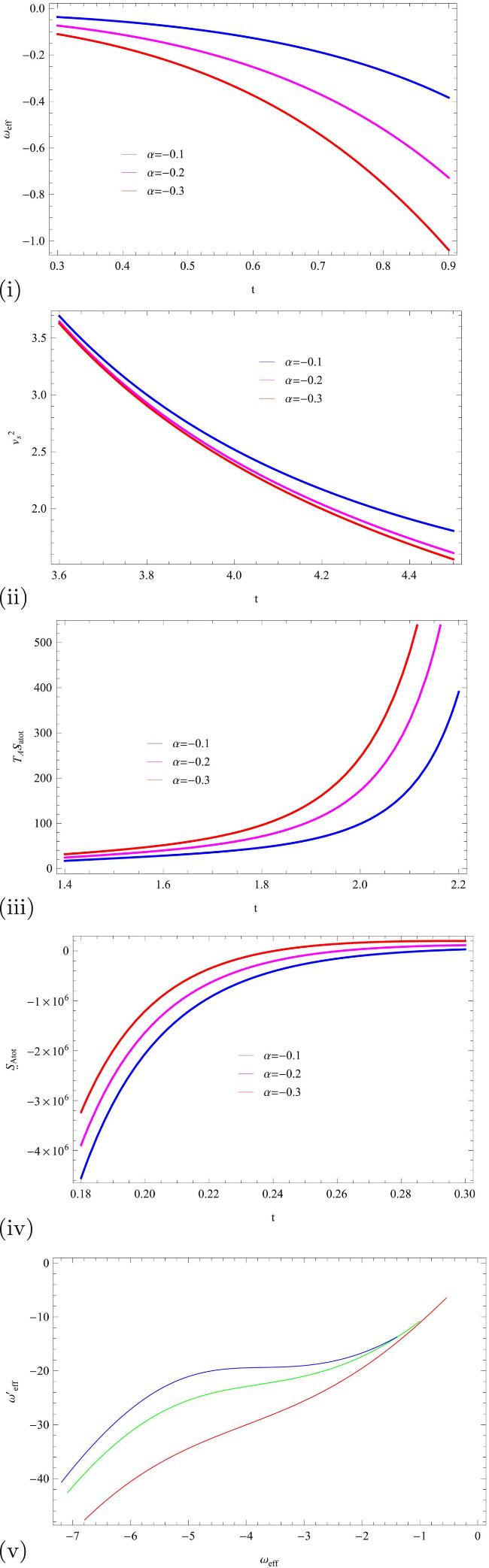
Figure 3. Plots of (i) The EoS parameter is plotted against cosmic time t, the plot exhibits the quintessence era, then transitioning to a cosmological constant phase and finally entering the phantom era. (ii) Squared speed of parameter as the function of t which lead to stability of the underlying model (iii) GSLT $({\dot{S}}_{\mathrm{tot}})$ versus t which corresponds to validity of GSLT $({\dot{S}}_{\mathrm{tot}}\gt 0)$ (iv) Thermal equilibrium which ensures the thermal stability of a system $({\ddot{S}}_{\mathrm{tot}}\lt 0)$ (v) The ${\omega }_{\mathrm{eff}}-{\omega }_{\mathrm{eff}}^{{\prime} }$ plane exhibits the freezing region. These plots are drawn for matter bounce cosmology. |
4.4. Little rip cosmology
The little rip cosmology offers a model of the Universe's evolution characterized by continuous accelerated expansion without the occurrence of a finite-time singularity. In contrast to the Big Rip scenario, where the scale factor, energy density and pressure experience infinite growth at a specific cosmic time ts, the little rip ensures that these parameters diverge only as t → ∞. This framework involves the EoS for DE evolving so that ω → -1 asymptotically, thereby avoiding singularities within any finite time. Consequently, this mechanism supports unbounded cosmic expansion while maintaining geodesic completeness and preventing crushing singularities. When considering future singularities, the Little Rip cosmology serves as a method to bypass them. Finite-time singularities, such as the Big Rip (Type I), Sudden Singularity (Type II), Big Freeze (Type III), and Generalized Sudden Singularity (Type IV), typically result in the divergence of parameters like the Hubble rate, scale factor, or their derivatives at a finite ts. The little rip framework, however, ensures that these quantities grow unbounded only as t → ∞, thus avoiding the geodesic incompleteness associated with finite-time singularities. This characteristic positions the Little Rip as a noteworthy alternative in the study of cosmic evolution.
This model also offers significant physical and observational relevance. In this scenario, the Hubble parameter H(t) increases indefinitely, leading to the gradual disintegration of gravitationally bound systems, including galaxies and atoms, due to intense tidal forces. Nonetheless, the asymptotic nature of the divergence prevents abrupt, catastrophic events. Additionally, the model's prediction that ω → -1 aligns well with observational data of Planck 2018 [60, 61], which suggests that DE behaves similarly to a cosmological constant. This makes the Little Rip cosmology a compelling theoretical framework for explaining the Universe's late-time accelerated expansion. For little rip cosmology, the scale factor is obtained as
$\begin{eqnarray}a(t)=B\exp \left(\frac{{f}_{0}}{\beta +1}{(t-{t}_{s})}^{\beta +1}\right),\end{eqnarray}$
where B > 0 expresses a dimensionless model parameter, ts is bouncing time and β is a constant which cannot be equal to -1, 0, 1. When t = ts then a(ts) = B while for t < ts and t > ts bounces are considered as future and past singularity respectively. Many bouncing cosmologies can be created by varying the value of β. Some types of singularities are following●If β < -1, the scale factor is diverging with finite time. Singularities of this type cause a dispersion of gravitationally bound structure and explain accelerated phase of cosmos [62].
●If β > 0, then a(t) is diverges infinitely many times that oppose to 1. These singularities also caused the dissociation of structure [63].
●If 0 < β < 1, it caused by diverging pressure. In such universes, there is a tremendous deceleration.
●If -1 < β < 0, this form of singularities arises when first and higher order of derivatives of a(t) diverges [64].
●If β > 1, in this type singularities occur because of divergence of higher order derivative of H(t) for n ≥ 2 [65].
Hubble parameter and their higher derivatives for this cosmology are given as
$\begin{eqnarray}\begin{array}{rcl}H & = & {f}_{0}{(t-{t}_{s})}^{\beta },\\ \dot{H} & = & \beta {f}_{0}{(t-{t}_{s})}^{\beta -1},\\ \ddot{H} & = & \beta (\beta -1){f}_{0}{(t-{t}_{s})}^{\beta -2},\\ \dddot{H} & = & \beta (\beta -1)(\beta -2){f}_{0}{(t-{t}_{s})}^{\beta -3},\\ \ddddot{H} & = & \beta (\beta -1)(\beta -2)(\beta -3){f}_{0}{(t-{t}_{s})}^{\beta -4}.\end{array}\end{eqnarray}$
The EoS parameter ωeff by taking into account equation (2.11 ) utilizing β = 0.50, f0 = 0.3, ts = 0.1, B = 1.5 and fit values of α as shown in figure 4(i). It is observed that the graph shows the quintessence phase initially, as t increases, crossing the cosmological constant and moving towards phantom phase. The positive values of ${v}_{s}^{2}$ that are described in figure 4(ii) mathematically illustrated in equation (A1 ) lead to stable behavior of little rip cosmology. The total rate of change of entropy is plotted in figure 4(iii) assuming apparent horizon as infrared cutoff. The trajectories of the plot are showing positive behavior which corresponding to the validity of GSLT. In figure 4(iv), the thermal equilibrium mathematically represented in equation (A4 ) expresses the system has obeyed this condition. For this cosmological bouncing the ${\omega }_{\mathrm{eff}}-{\omega }_{\mathrm{eff}}^{{\prime} }$ plane corresponds to thawing region as for ωeff < 0 leads to ${\omega }_{\mathrm{eff}}^{{\prime} }\gt 0$.
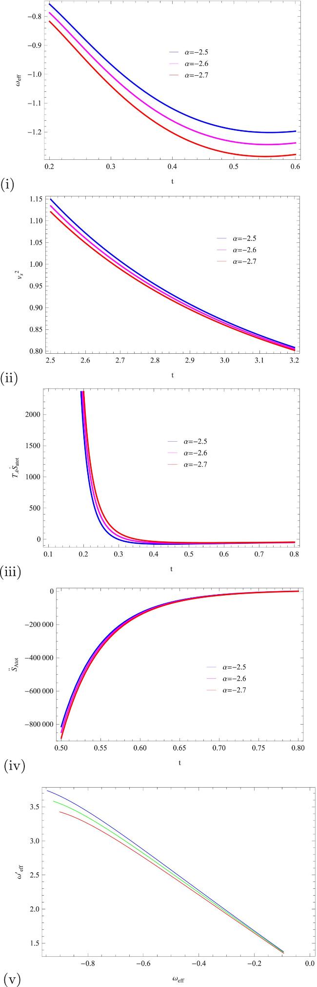
Figure 4. Plots of (i) The EoS parameter is plotted against cosmic time t, the plot illustrates the evolution the quintessence era, then transitioning to a cosmological constant phase and finally entering the phantom era. (ii) Squared speed of parameter as the function of t which lead to stability of the underlying model (iii) GSLT $({\dot{S}}_{\mathrm{tot}})$ versus t which corresponds to validity of GSLT $({\dot{S}}_{\mathrm{tot}}\gt 0)$ (iv) Thermal equilibrium which ensures the thermal stability of a system $({\ddot{S}}_{\mathrm{tot}}\lt 0)$ (v) The ${\omega }_{\mathrm{eff}}-{\omega }_{\mathrm{eff}}^{{\prime} }$ plane exhibits the thawing region. These plots are drawn for little rip cosmology. |
4.5. Superbounce cosmology
Next, we consider superbounce cosmology [66] and it is used to create a cosmos which might collapse and emerge after big bang without singularity [30]. This type of cosmology having power law scale factor as
$\begin{eqnarray}a(t)={\left(\frac{{t}_{q}-t}{{t}_{0}}\right)}^{\frac{2}{{d}^{2}}},\end{eqnarray}$
where tq expresses the time when bounce occurs while t0 denotes the arbitrary time, d2 > 6 is real constant. In this case the expression of H(t) is given by $\begin{eqnarray}H=\frac{2}{{d}^{2}}{(t-{t}_{q})}^{-1},\end{eqnarray}$
which recognize the exitance of bounce when t = tq. We can observe the signature of Hubble parameter varies before and after the bounce but there is singularity at the bounce point. $\begin{eqnarray}\begin{array}{rcl}\dot{H} & = & -\frac{2}{{d}^{2}}{(t-{t}_{q})}^{-2},\\ \ddot{H} & = & \frac{4}{{d}^{2}}{(t-{t}_{q})}^{-3},\\ \dddot{H} & = & -\frac{12}{{d}^{2}}{(t-{t}_{q})}^{-4},\\ \ddddot{H} & = & \frac{48}{{d}^{2}}{(t-{t}_{q})}^{-5}.\end{array}\end{eqnarray}$
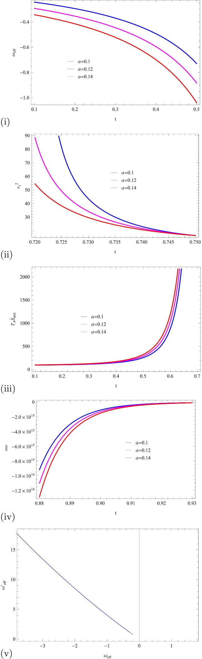
Now, we utilized the mathematical model equation (2.11 ) to evaluate the effective EoS parameter with d2 = 6.8, t0 = 0.0020, tq = 0.75 and different values of α as plotted in figure 5(i). The graph shows the evolution from the vacuum phase to the quintessence phase by increasing the value of parameter t. From figure 5(ii), we can see the squared speed of sound describes the stability of superbouncing cosmology. The GSLT which has mathematical relation equation (A3 ) with Bekenstein entropy at apparent horizon is indicated figure 5(iii) that yields GSLT is stable for this model. The graphical behavior of thermal equilibrium is presented in figure 5(iv) using equation (A4 ). The behavior of this plot leads the system that is in thermal equilibrium. For this cosmological bouncing the ${\omega }_{\mathrm{eff}}-{\omega }_{\mathrm{eff}}^{{\prime} }$ plane corresponds to thawing region as for ωeff < 0 leads to ${\omega }_{\mathrm{eff}}^{{\prime} }\gt 0$.
Figure 5. Plots of (i) The EoS parameter is plotted against cosmic time t, the plot illustrates the evolution the quintessence era, then transitioning to a cosmological constant phase and finally entering the phantom era. (ii) Squared speed of parameter as the function of t which lead to stability of the underlying model (iii) GSLT $({\dot{S}}_{\mathrm{tot}})$ versus t which corresponds to validity of GSLT $({\dot{S}}_{\mathrm{tot}}\gt 0)$ (iv) Thermal equilibrium which ensures the thermal stability of a system $({\ddot{S}}_{\mathrm{tot}}\lt 0)$ (v) The ${\omega }_{{\rm{e}}\rm{f}{\rm{f}}}-{\omega }_{\mathrm{eff}}^{{\prime} }$ plane exhibits the thawing region. These plots are drawn for superbouncing cosmology. |
5. Conclusion
In this paper, we have worked on cosmic and thermodynamic aspects under modified theory gravity as f(R, A) theory taking flat FRW universe. For this purpose, we have to assumed several kinds of bouncing scenarios such as symmetric bounce cosmology, oscillatory bounce cosmology, matter bounce cosmology, little rip cosmology and superbounce cosmology. We have to reconstruct these models and discuss effective EoS parameter, squared speed of sound parameter, GSLT and thermal equilibrium condition graphically versus t. This work is significant because it provides a comprehensive analysis of cosmic evolution and thermodynamic stability within the framework of f(R, A) gravity, incorporating various bouncing cosmologies. Unlike previous studies on modified gravity, this research explores the role of the anticurvature term in ensuring stable cosmic evolution, demonstrating its impact on the EoS parameter, stability conditions, and the generalized second law of thermodynamics. The results indicate that f(R, A) gravity can successfully describe bouncing scenarios while maintaining thermodynamic consistency, offering a viable alternative to standard f(R) and f(R, T) theories. Potential applications of this model extend to early universe physics, where it may provide a framework for resolving singularity issues and contribute to alternative inflationary models. Future work could involve a detailed parameter-space analysis to refine constraints by using observational data of Planck 2018 [60, 61]. Additionally, extending the study to include perturbation analysis and large-scale structure formation could further validate the cosmological viability of f(R, A) gravity. The results are summarized in the following and as well as in the table 1:
Table 1. Comparison of various cosmological bouncing models. |
| Cosmologies | ωeff | ${v}_{s}^{2}$ | ${T}_{A}{\dot{S}}_{A\mathrm{tot}}$ | ${\ddot{S}}_{A\mathrm{tot}}$ |
|---|---|---|---|---|
| Symmetric Bounce | Phantom Phase | Stable | Valid | Valid |
| | ||||
| Oscillatory Bounce | Quintessence | Stable | Valid | Valid |
| | ||||
| Matter Bounce | Phantom Phase | Stable | Valid | Valid |
| | ||||
| Little Rip | Phantom Phase | Stable | Valid | Valid |
| | ||||
| Superbounce | Phantom Phase | Stable | Valid | Valid |
●For symmetric bounce cosmology. We considered the symmetric bounce cosmology whose scale factor is $a(t)=B\exp (\tfrac{\beta {t}^{2}}{{t}_{p}^{2}})$ and discussed the evolution of the Universe. First, we find effective EoS parameter for this cosmology and found the Universe is in the transition phase. We found that the Universe is in the quintessence phase for 0.1 < t < 0.35 then entering into the cosmological constant era when ωeff = -1. It is also interesting to mention here that at t > 0.36 the Universe is under the influence of the phantom-dominated era. Next, we found the squared speed of sound parameter to check the stability of the model. We can see that $0\lt {v}_{s}^{2}\lt 1$ for the selected range of t which leads to the stability of the model (figure 1(ii)). Furthermore, in figure 1(iii), we plot the trajectories of GSLT w.r.t. t and found positive behavior which corresponds to the validity of GSLT. We found the thermal equilibrium condition for this bouncing cosmology which also showed consistent behavior. For this cosmological bouncing the ${\omega }_{\mathrm{eff}}-{\omega }_{\mathrm{eff}}^{{\prime} }$ plane corresponds to thawing region as ωeff < 0 leads to ${\omega }_{\mathrm{eff}}^{{\prime} }\gt 0$.
●Oscillatory bouncing cosmology. Next, we considered oscillatory bouncing cosmology whose scale factor is defined as $a(t)=B{\sin }^{2}\left(\frac{Ct}{{t}_{s}}\right)$. Firstly, we plot the EoS parameter (figure 2(i)) for this cosmology and found the quintessence behavior of universe. The plot of squared speed of sound parameter corresponds to stability of the underlying model as ${v}_{s}^{2}\gt 0$ (figure 2(ii)). The condition for the validity of the GSLT has been found using the positivity of ${\dot{S}}_{A\mathrm{tot}}$. In figure 2(iv), we obtained the consistent condition of thermal equilibrium. For this model, the ${\omega }_{\mathrm{eff}}-{\omega }_{\mathrm{eff}}^{{\prime} }$ plane corresponds to freezing region as for ωeff < 0 we obtain ${\omega }_{\mathrm{eff}}^{{\prime} }\lt 0$.
●Matter bounce cosmology. The scale factor for this cosmology is given as $a(t)=B{\left(\frac{3}{2}{\rho }_{0}{t}^{2}+1\right)}^{\frac{1}{3}}$. The behavior of EoS parameter can be observed in figure 3(i). In particular, the EoS parameter for the matter bounce cosmology varies in the quintessence as well as cosmological constant region for different values of the model parameter α. We also addressed the behavior of ${v}_{s}^{2}$ for this bouncing cosmology and found the positive range. Moreover, we have examined the viability of the GSLT. After a careful mathematical analysis, we have found ${\dot{S}}_{A\mathrm{tot}}\gt 0$ which leads to the validity of GSLT. On the other hand, for thermal equilibrium condition, we obtained ${\ddot{S}}_{A\mathrm{tot}}\lt 0$ which fulfilled the required condition. For this cosmological bouncing the ${\omega }_{\mathrm{eff}}-{\omega }_{\mathrm{eff}}^{{\prime} }$ plane corresponds to freezing region as for ωeff < 0 leads to ${\omega }_{\mathrm{eff}}^{{\prime} }\lt 0$.
●Little rip cosmology. We then repeat the above analysis for little rip cosmology whose scale factor is obtained as $a(t)=B\exp (\tfrac{{f}_{0}}{\beta +1}{(t-{t}_{s})}^{\beta +1})$. We have plotted the evolutionary curves of EoS parameter for this model in figure 4(i). we found the quintessence, cosmological constant and phantom era for different stages of time. Next, we found ${v}_{s}^{2}\gt 0$, ${\dot{S}}_{A\mathrm{tot}}\gt 0$ and ${\ddot{S}}_{A\mathrm{tot}}\lt 0$ (figures 4(i), (ii), (iii)). All these constraints favor the validity of the required conditions. The ${\omega }_{\mathrm{eff}}-{\omega }_{\mathrm{eff}}^{{\prime} }$ plane corresponds to thawing region as for ωeff < 0 leads to ${\omega }_{\mathrm{eff}}^{{\prime} }\gt 0$.
●Superbounce cosmology. The same analysis is found for superbounce cosmology whose scale factor is given as $a(t)={\left(\frac{{t}_{q}-t}{{t}_{0}}\right)}^{\frac{2}{{d}^{2}}}$. We also found the consistent results for this cosmology (figures 5(i),(ii),(iii),(iv)). The ${\omega }_{\mathrm{eff}}-{\omega }_{\mathrm{eff}}^{{\prime} }$ plane corresponds to thawing region as for ωeff < 0 leads to ${\omega }_{\mathrm{eff}}^{{\prime} }\gt 0$.
It is interesting to mention here that our results regarding ωeff and ${\omega }_{\mathrm{eff}}-{\omega }_{\mathrm{eff}}^{{\prime} }$ in all cases of scale factor are consistent with recent observational data as displayed in tables 2 and 3, respectively. In [67], authors explored f(G, T2) gravity by coupling the Gauss-Bonnet invariant with the energymomentum squared term. Various bouncing cosmological models are analyzed, showing stability and avoiding singularities. The results supported a viable alternative to Big Bang cosmology, aligning with observational constraints. Koussour and Myrzakulov [68], examined bouncing cosmologies in symmetric teleparallel f(Q) gravity, analyzing stability through energy conditions and perturbations. The results indicated initial instability but overall stability, with the EoS crossing the phantom divide near the bounce, supported a viable non-singular cosmic evolution. Furthermore, the bouncing cosmological models are examined in the framework of f(Q, T) gravity [69]. By analyzing different bouncing scenarios such as symmetric, super, oscillatory, matter, and exponential bounce models, the paper evaluates the behavior of key cosmological parameters, energy conditions, and perturbations. The results indicate that these models can describe cosmic evolution while avoiding singularities, providing insights into early and late-time universe dynamics.
Table 2. Summary of the observational data of Planck 2018 on ωeff. |
Table 3. Observational data of Planck 2018 for ${\omega }_{\mathrm{eff}}-{\omega }_{\mathrm{eff}}^{{\prime} }$ [60, 61]. |
| ωeff | ${\omega }_{\mathrm{eff}}^{{\prime} }$ | Observational datasets |
|---|---|---|
| $-1.13{\pm }_{0.25}^{0.24}$ | <1.32 | BAO+WP+BAO |
| | ||
| -1.13 ± 0.18 | 0.85 ± 0.47 | WMAP+eCAMB+BAO+H0 |
| | ||
| $-1.13{\pm }_{0.25}^{0.24}$ | $-0.85{\pm }_{0.49}^{0.50}$ | WMAP+eCAMB+BAO+H0+SNe |
In the context of f(R, A) gravity, antisymmetric tensors, including the Levi-Civita symbols, play a critical role in constructing invariants that enhance the gravitational framework. Although it is known that such constructions may lead to ghost instabilities in certain models, the specific formulation f(R, A) = R + αA-1 circumvents these issues. This is achieved due to the following reasons:
●The antisymmetric nature of the Levi-Civita symbols guarantees that the resulting invariants adhere to the symmetry principles of spacetime.
●The functional structure of f(R, A), along with the derived field equations, is intentionally designed to be second-order, thereby avoiding the higher-order derivative terms that are commonly linked to ghost instabilities.